SlideShare a Scribd company logo
Program and Network Properties
• Conditions of parallelism
• Program partitioning and scheduling
• Program flow mechanisms
• System interconnect architectures
2
Conditions of Parallelism
The exploitation of parallelism in computing requires un
derstanding the basic theory associated with it. Progress
is needed in several areas:
computation models for parallel computing
interprocessor communication in parallel architectures
integration of parallel systems into general environments
3
Data dependences
The ordering relationship between statements is indicated by the data de
pendence.
•Flow dependence
•Anti dependence
•Output dependence
•I/O dependence
•Unknown dependence
4
Data Dependence - 1
• Flow dependence: S1 precedes S2, and at least one output of S1 is
input to S2.
• Antidependence: S1 precedes S2, and the output of S2 overlaps th
e input to S1.
• Output dependence: S1 and S2 write to the same output variable.
• I/O dependence: two I/O statements (read/write) reference the sa
me variable, and/or the same file.
5
Data dependence example
S1: Load R1, A
S2: Add R2, R1
S3: Move R1, R3
S4: Store B, R1
S1
S2 S4
S3
6
I/O dependence example
S1: Read (4), A(I)
S2: Rewind (4)
S3: Write (4), B(I)
S4: Rewind (4)
S1 S3I/O
7
Control dependence
• The order of execution of statements cannot be determined before ru
n time
o Conditional branches
o Successive operations of a looping procedure
8
Control dependence examples
Do 20 I = 1, N
A(I) = C(I)
IF(A(I) .LT. 0) A(I)=1
20 Continue
Do 10 I = 1, N
IF(A(I-1) .EQ. 0) A(I)=0
10 Continue
9
Resource dependence
• Concerned with the conflicts in using shared resources
o Integer units
o Floating-point units
o Registers
o Memory areas
o ALU
o Workplace storage
10
Bernstein’s conditions
• Set of conditions for two processes to execute in parallel
I1 O2 = Ø
I2 O1 = Ø
O1 O2 = Ø
11
Bernstein’s Conditions - 2
• In terms of data dependencies, Bernstein’s conditions imply th
at two processes can execute in parallel if they are flow-indepe
ndent, anti-independent, and output-independent.
• The parallelism relation || is commutative (Pi || Pj implies Pj ||
Pi ), but not transitive (Pi || Pj and Pj || Pk does not imply Pi ||
Pk ) . Therefore, || is not an equivalence relation.
• Intersection of the input sets is allowed.
12
Utilizing Bernstein’s conditions
P1 : C = D x E
P2 : M = G + C
P3 : A = B + C
P4 : C = L + M
P5 : F = G / E
P1
P3
P2 P4
P5
13
Utilizing Bernstein’s conditions
14
Hardware parallelism
• A function of cost and performance tradeoffs
• Displays the resource utilization patterns of simultan
eously executable operations
• Denote the number of instruction issues per machin
e cycle: k-issue processor
• A multiprocessor system with n k-issue processors s
hould be able to handle a maximum number of nk th
reads of instructions simultaneously
15
Software parallelism
• Defined by the control and data dependence of p
rograms
• A function of algorithm, programming style, and
compiler organization
• The program flow graph displays the patterns of
simultaneously executable operations
16
Mismatch between software and hardware parallelism - 1
L1 L2 L3 L4
X1 X2
+ -
A B
Fig. : Software parallelism
Cycle 1
Cycle 2
Cycle 3
Maximum software parallelis
m (L=load, X/+/- = arithmeti
c)
8 instructions(4 loads and 4
arithmetic operations )
Parallelism varies from 4 to
2 in three cycles
17
Mismatch between software and hardware parall
elism - 2
L1
L2
L4
L3X1
X2
+
-
A
B
Cycle 1
Cycle 2
Cycle 3
Cycle 4
Cycle 5
Cycle 6
Cycle 7
Same problem, but consid
ering the parallelism on a
two-issue superscalar pro
cessor.
18
Mismatch between software and hardware parall
elism - 3
L1
L2
S1
X1
+
L5
L3
L4
S2
X2
-
L6
BA
Cycle 1
Cycle 2
Cycle 3
Cycle 4
Cycle 5
Cycle 6
Same problem, w
ith two single-iss
ue processors
= inserted for s
ynchronization
Fig. : Dual processor execution
19
Types of Software Parallelism
• Control Parallelism – two or more operations can be performed s
imultaneously. This can be detected by a compiler, or a programmer
can explicitly indicate control parallelism by using special language c
onstructs or dividing a program into multiple processes.
• Data parallelism – multiple data elements have the same operatio
ns applied to them at the same time. This offers the highest potentia
l for concurrency (in SIMD and MIMD modes). Synchronization in
SIMD machines handled by hardware.
20
Solving the Mismatch Problems
• Develop compilation support
• Redesign hardware for more efficient exploitation by compilers
• Use large register files and sustained instruction pipelining.
• Have the compiler fill the branch and load delay slots in code genera
ted for RISC processors.
21
The Role of Compilers
• Compilers used to exploit hardware features to improve performanc
e.
• Interaction between compiler and architecture design is a necessity i
n modern computer development.
• It is not necessarily the case that more software parallelism will impr
ove performance in conventional scalar processors.
• The hardware and compiler should be designed at the same time.
22
Program Partitioning & Scheduling
• The size of the parts or pieces of a program that can be considered fo
r parallel execution can vary.
• The sizes are roughly classified using the term “granule size,” or sim
ply “granularity.”
• The simplest measure, for example, is the number of instructions in
a program part.
• Grain sizes are usually described as fine, medium or coarse, dependi
ng on the level of parallelism involved.
23
Latency
• Latency is the time required for communication between different s
ubsystems in a computer.
• Memory latency, for example, is the time required by a processor to
access memory.
• Synchronization latency is the time required for two processes to sy
nchronize their execution.
• Computational granularity and communication latency are closely re
lated.
24
Levels of Parallelism
Jobs or programs
Instructions
or statements
Non-recursive loops
or unfolded iterations
Procedures, subroutines,
tasks, or coroutines
Subprograms, job steps or
related parts of a program
}
}
Coarse grain
Medium grain
}Fine grain
Increasing com
munication dem
and and scheduli
ng overhead
Higher degree of
parallelism
25
Instruction Level Parallelism
• This fine-grained, or smallest granularity level typically involves less
than 20 instructions per grain. The number of candidates for paralle
l execution varies from 2 to thousands, with about five instructions o
r statements (on the average) being the average level of parallelism.
• Advantages:
o There are usually many candidates for parallel execution
o Compilers can usually do a reasonable job of finding this parallelism
26
Loop-level Parallelism
• Typical loop has less than 500 instructions.
• If a loop operation is independent between iterations, it can be handl
ed by a pipeline, or by a SIMD machine.
• Most optimized program construct to execute on a parallel or vector
machine
• Some loops (e.g. recursive) are difficult to handle.
• Loop-level parallelism is still considered fine grain computation.
27
Procedure-level Parallelism
• Medium-sized grain; usually less than 2000 instructions.
• Detection of parallelism is more difficult than with smaller grains; in
terprocedural dependence analysis is difficult and history-sensitive.
• Communication requirement less than instruction-level
• SPMD (single procedure multiple data) is a special case
• Multitasking belongs to this level.
28
Subprogram-level Parallelism
• Job step level; grain typically has thousands of instructions; medium
- or coarse-grain level.
• Job steps can overlap across different jobs.
• Multiprograming conducted at this level
• No compilers available to exploit medium- or coarse-grain parallelis
m at present.
29
Job or Program-Level Parallelism
• Corresponds to execution of essentially independent jobs or program
s on a parallel computer.
• This is practical for a machine with a small number of powerful proc
essors, but impractical for a machine with a large number of simple
processors (since each processor would take too long to process a sin
gle job).
30
Communication Latency
• Balancing granularity and latency can yield better performance.
• Various latencies attributed to machine architecture, technology, an
d communication patterns used.
• Latency imposes a limiting factor on machine scalability. Ex. Memo
ry latency increases as memory capacity increases, limiting the amou
nt of memory that can be used with a given tolerance for communica
tion latency.
31
Interprocessor Communication Latency
• Needs to be minimized by system designer
• Affected by signal delays and communication patterns
• Ex. n communicating tasks may require n (n - 1)/2 communication li
nks, and the complexity grows quadratically, effectively limiting the
number of processors in the system.
32
Grain Packing and Scheduling
• Two questions:
o How can I partition a program into parallel “pieces” to yield the shorte
st execution time?
o What is the optimal size of parallel grains?
• There is an obvious tradeoff between the time spent scheduling and
synchronizing parallel grains and the speedup obtained by paralle
l execution.
• Solution is both problem-dependent and machine-dependent.
• Goal is to produce a short schedule for fast execution of subdivided prog
ram modules.
• One approach to the problem is called “grain packing”
33
Program Graphs and Packing
• A program graph is similar to a dependence graph
o Nodes = { (n,s) }, where n = node name, s = size (larger s = larger grain siz
e).
o Edges = { (v,d) }, where v = variable being “communicated,” and d = com
munication delay.
• Packing two (or more) nodes produces a node with a larger grain siz
e and possibly more edges to other nodes.
• Packing is done to eliminate unnecessary communication dela
ys or reduce overall scheduling overhead.
34EENG-630 - Chapter 2
35
Scheduling
• A schedule is a mapping of nodes to processors and start times such
that communication delay requirements are observed, and no two n
odes are executing on the same processor at the same time.
• Some general scheduling goals
o Schedule all fine-grain activities in a node to the same processor to minim
ize communication delays.
o Select grain sizes for packing to achieve better schedules for a particular p
arallel machine.
36
Scheduling (Cont)
37
Static multiprocessor scheduling
• Grain packing may not be optimal
• Dynamic multiprocessor scheduling is an NP-hard problem
• Node duplication is a static scheme for multiprocessor scheduling
38
Node duplication
• Duplicate some nodes to eliminate idle time and reduce communicat
ion delays
• Grain packing and node duplication are often used jointly to determi
ne the best grain size and corresponding schedule
39
Schedule without node duplication
A,4
a,1
b,1 c,8
a,8
c,1
C,1B,1
D,2 E,2
e,4d,4
P1 P2 P2P1
A
D
B
I
E
C
I4
6
13
21
27
23
20
16
14
12
4
40
Schedule with node duplication
A,4
a,1
b,1 c,1
a,1
c,1
C’,1B,1
D,2 E,2
P1 P2 P2P1
A
D
B
E
C
A
4
6
10
14
13
9
6
4
C,1
A’,4
a,1
C
7
41
Grain determination and scheduling optimization
Step 1: Construct a fine-grain program graph
Step 2: Schedule the fine-grain computation
Step 3: Grain packing to produce coarse grains
Step 4: Generate a parallel schedule based on the packed graph
42
System Interconnect Architectures
• Direct networks for static connections
• Indirect networks for dynamic connections
• Networks are used for
o internal connections in a centralized system among
• processors
• memory modules
• I/O disk arrays
o distributed networking of multicomputer nodes
43
Goals and Analysis
• The goals of an interconnection network are to provide
o low-latency
o high data transfer rate
o wide communication bandwidth
• Analysis includes
o latency
o bisection bandwidth
o data-routing functions
o scalability of parallel architecture
44
Network Properties and Routing
• Static networks: point-to-point direct connections that will not chan
ge during program execution
• Dynamic networks:
o switched channels dynamically configured to match user program commu
nication demands
o include buses, crossbar switches, and multistage networks
• Both network types also used for inter-PE data routing in SIMD com
puters
45
Network Parameters
• Network size: The number of nodes (links or channels) in the graph
used to represent the network
• Node Degree d: The number of edges incident to a node. In the case
of unidirectional channels, the number of channels into a node is t
he in degree and that out of a node is the out degree. Then the
node degree is the sum of the two.
• Network Diameter D: The maximum shortest path between any two
nodes
46
Network Parameters (cont.)
• Bisection Width:
o Channel bisection width b: The minimum number of edges (channels)
along the cut that divides the network in two equal halves
o Each channel has w bit wires
o Wire bisection width: B=b*w; B is the wiring density of the network. It
provides a good indicator of the max communication bandwidth along the
bisection of the network
47
Terminology - 1
• Network usually represented by a graph with a finite nu
mber of nodes linked by directed or undirected edges.
• Number of nodes in graph = network size .
• Number of edges (links or channels) incident on a node =
node degree d (also note in and out degrees when edges a
re directed). Node degree reflects number of I/O ports as
sociated with a node, and should ideally be small and con
stant.
• Diameter D of a network is the maximum shortest path b
etween any two nodes, measured by the number of links t
raversed; this should be as small as possible (from a com
munication point of view).
48
Terminology - 2
• Channel bisection width b = minimum number of edges cut
to split a network into two parts each having the same numb
er of nodes. Since each channel has w bit wires, the wire bis
ection width B = bw. Bisection width provides good indicati
on of maximum communication bandwidth along the bisecti
on of a network, and all other cross sections should be boun
ded by the bisection width.
• Wire (or channel) length = length (e.g. weight) of edges bet
ween nodes.
• Network is symmetric if the topology is the same looking fro
m any node; these are easier to implement or to program.
• Other useful characterizing properties: homogeneous nodes
? buffered channels? nodes are switches?
49
Data Routing Functions
Data-routing network used for inter-PE data exchange. This network ca
n be static (i.e: hypercube) or dynamic (i.e: multistage network)
Commonly data-routing functions includes:
• Shifting
• Rotating
• Permutation (one to one)
• Broadcast (one to all)
• Multicast (many to many)
• Personalized broadcast (one to many)
• Shuffle
• Exchange
• Etc.
50
Hypercube Routing Functions
• If the vertices of a n-dimensional cube are labeled with n-bit number
s so that only one bit differs between each pair of adjacent vertices, t
hen n routing functions are defined by the bits in the node (vertex) a
ddress.
• For example, with a 3-dimensional cube, we can easily identify routi
ng functions that exchange data between nodes with addresses that
differ in the least significant, most significant, or middle bit.
• Figure: 2.15
51
Factors Affecting Network Performance
• Functionality – how the network supports data routing, interrupt
handling, synchronization, request/message combining, and cohere
nce
• Network latency – worst-case time for a unit message to be transf
erred
• Bandwidth – maximum data rate
• Hardware complexity – implementation costs for wire, logic, swi
tches, connectors, etc.
• Scalability – how easily does the scheme adapt to an increasing nu
mber of processors, memories, etc.?
52
Static Networks
• Linear Array
• Ring and Chordal Ring
• Barrel Shifter
• Tree and Star
• Fat Tree
• Mesh and Torus
53
Static Networks – Linear Array
• N nodes connected by n-1 links (not a bus); segments between differ
ent pairs of nodes can be used in parallel.
• Internal nodes have degree 2; end nodes have degree 1.
• Diameter = n-1
• Bisection = 1
• For small n, this is economical, but for large n, it is obviously inappr
opriate.
54
Static Networks – Ring, Chordal Ring
• Like a linear array, but the two end nodes are connected by an n th li
nk; the ring can be uni- or bi-directional. Diameter is n/2 for a b
idirectional ring, or n for a unidirectional ring.
• By adding additional links (e.g. “chords” in a circle), the node degree
is increased, and we obtain a chordal ring. This reduces the network
diameter.
• In the limit, we obtain a fully-connected network, with a node degree
of n -1 and a diameter of 1.
55
Static Networks – Barrel Shifter
• Like a ring, but with additional links between all pairs of nodes that
have a distance equal to a power of 2.
• With a network of size N = 2n, each node has degree d = 2n -1, and th
e network has diameter D = n /2.
• Barrel shifter connectivity is greater than any chordal ring of lower n
ode degree.
• Barrel shifter much less complex than fully-interconnected network.
56
57
Static Networks – Tree and Star
• A k-level completely balanced binary tree will have N = 2k – 1 nodes,
with maximum node degree of 3 and network diameter is 2(k – 1).
• The balanced binary tree is scalable, since it has a constant maximu
m node degree.
• A star is a two-level tree with a node degree d = N – 1 and a constant
diameter of 2.
58
Static Networks – Fat Tree
• A fat tree is a tree in which the number of edges between nodes incre
ases closer to the root (similar to the way the thickness of limbs incre
ases in a real tree as we get closer to the root).
• The edges represent communication channels (“wires”), and since co
mmunication traffic increases as the root is approached, it seems log
ical to increase the number of channels there.
59
Static Networks – Mesh and Torus
• Pure mesh – N = n k nodes with links between each adjacent pair of
nodes in a row or column (or higher degree). This is not a symmetri
c network; interior node degree d = 2k, diameter = k (n – 1).
• Illiac mesh (used in Illiac IV computer) – wraparound is allowed, th
us reducing the network diameter to about half that of the equivalent
pure mesh.
• A torus has ring connections in each dimension, and is symmetric.
An n n binary torus has node degree of 4 and a diameter of 2 n
/ 2 .
60
Static Networks – Systolic Array
• A systolic array is an arrangement of processing elements and comm
unication links designed specifically to match the computation and c
ommunication requirements of a specific algorithm (or class of algor
ithms).
• This specialized character may yield better performance than more g
eneralized structures, but also makes them more expensive, and mor
e difficult to program.
61
Network Throughput
• Network throughput – number of messages a network can handle in
a unit time interval.
• One way to estimate is to calculate the maximum number of message
s that can be present in a network at any instant (its capacity); throu
ghput usually is some fraction of its capacity.
• A hot spot is a pair of nodes that accounts for a disproportionately la
rge portion of the total network traffic (possibly causing congestion).
• Hot spot throughput is maximum rate at which messages can be sen
t between two specific nodes.
62
Dynamic Connection Networks
• Dynamic connection networks can implement all communication pa
tterns based on program demands.
• In increasing order of cost and performance, these include
o bus systems
o multistage interconnection networks
o crossbar switch networks
• Price can be attributed to the cost of wires, switches, arbiters, and co
nnectors.
• Performance is indicated by network bandwidth, data transfer rate,
network latency, and communication patterns supported.
63
Dynamic Networks – Bus Systems
• A bus system (contention bus, time-sharing bus) has
o a collection of wires and connectors
o multiple modules (processors, memories, peripherals, etc.) which con
nect to the wires
o data transactions between pairs of modules
• Bus supports only one transaction at a time.
• Bus arbitration logic must deal with conflicting requests.
• Lowest cost and bandwidth of all dynamic schemes.
• Many bus standards are available.
64
Dynamic Networks – Switch Modules
• An a b switch module has a inputs and b outputs. A binary switch
has a = b = 2.
• It is not necessary for a = b, but usually a = b = 2k, for some integer k
.
• In general, any input can be connected to one or more of the outputs
. However, multiple inputs may not be connected to the same output
.
• When only one-to-one mappings are allowed, the switch is called a c
rossbar switch.
65
Multistage Networks
• In general, any multistage network is comprised of a collection of a
b switch modules and fixed network modules. The a b s
witch modules are used to provide variable permutation or other
reordering of the inputs, which are then further reordered by the
fixed network modules.
• A generic multistage network consists of a sequence alternating
dynamic switches (with relatively small values for a and b) with st
atic networks (with larger numbers of inputs and outputs). The stati
c networks are used to implement interstage connections (ISC).
66
Omega Network
• A 2 2 switch can be configured for
o Straight-through
o Crossover
o Upper broadcast (upper input to both outputs)
o Lower broadcast (lower input to both outputs)
o (No output is a somewhat vacuous possibility as well)
• With four stages of eight 2 2 switches, and a static perf
ect shuffle for each of the four ISCs, a 16 by 16 Omega net
work can be constructed (but not all permutations are po
ssible).
• In general , an n-input Omega network requires log 2 n st
ages of 2 2 switches and n / 2 switch modules.
67
68
Baseline Network
• A baseline network can be shown to be topologically equivalent to ot
her networks (including Omega), and has a simple recursive generati
on procedure.
• Stage k (k = 0, 1, …) is an m m switch block (where m = N / 2k ) co
mposed entirely of 2 2 switch blocks, each having two configuratio
ns: straight through and crossover.
69
4 4 Baseline Network
70
Crossbar Networks
• A m n crossbar network can be used to provide a constant latency con
nection between devices; it can be thought of as a single stage switch.
• Different types of devices can be connected, yielding different constraint
s on which switches can be enabled.
o With m processors and n memories, one processor may be able to generate request
s for multiple memories in sequence; thus several switches might be set in the same
row.
o For m m interprocessor communication, each PE is connected to both an input a
nd an output of the crossbar; only one switch in each row and column can be turne
d on simultaneously. Additional control processors are used to manage the crossba
r itself.

More Related Content

What's hot (20)

PPT
Hardware and Software parallelism
prashantdahake
 
PPTX
Architectural Development Tracks
ANJALIG10
 
PPTX
Multivector and multiprocessor
Kishan Panara
 
PDF
Parallel Algorithms
Dr Sandeep Kumar Poonia
 
PPT
multiprocessors and multicomputers
Pankaj Kumar Jain
 
PPT
Introduction to parallel_computing
Mehul Patel
 
PPT
advanced computer architesture-conditions of parallelism
Pankaj Kumar Jain
 
PDF
Aca2 01 new
Sumit Mittu
 
PPTX
Distributed computing
shivli0769
 
PPTX
Pram model
MANASYJAYASURYA
 
DOCX
Parallel computing persentation
VIKAS SINGH BHADOURIA
 
PPT
hierarchical bus system
Elvis Jonyo
 
PDF
Parallel programming model, language and compiler in ACA.
MITS Gwalior
 
DOCX
Amdahl`s law -Processor performance
COMSATS Institute of Information Technology
 
PPTX
Distributed shred memory architecture
Maulik Togadiya
 
PDF
Introduction to Parallel Computing
Akhila Prabhakaran
 
PPTX
System interconnect architecture
Gagan Kumar
 
PPT
Query Decomposition and data localization
Hafiz faiz
 
PDF
Lecture 1 introduction to parallel and distributed computing
Vajira Thambawita
 
PPTX
Parallel Programing Model
Adlin Jeena
 
Hardware and Software parallelism
prashantdahake
 
Architectural Development Tracks
ANJALIG10
 
Multivector and multiprocessor
Kishan Panara
 
Parallel Algorithms
Dr Sandeep Kumar Poonia
 
multiprocessors and multicomputers
Pankaj Kumar Jain
 
Introduction to parallel_computing
Mehul Patel
 
advanced computer architesture-conditions of parallelism
Pankaj Kumar Jain
 
Aca2 01 new
Sumit Mittu
 
Distributed computing
shivli0769
 
Pram model
MANASYJAYASURYA
 
Parallel computing persentation
VIKAS SINGH BHADOURIA
 
hierarchical bus system
Elvis Jonyo
 
Parallel programming model, language and compiler in ACA.
MITS Gwalior
 
Amdahl`s law -Processor performance
COMSATS Institute of Information Technology
 
Distributed shred memory architecture
Maulik Togadiya
 
Introduction to Parallel Computing
Akhila Prabhakaran
 
System interconnect architecture
Gagan Kumar
 
Query Decomposition and data localization
Hafiz faiz
 
Lecture 1 introduction to parallel and distributed computing
Vajira Thambawita
 
Parallel Programing Model
Adlin Jeena
 

Similar to Lec 4 (program and network properties) (20)

PPT
programnetwork_properties-parallelism_ch2.ppt
Jatin1071
 
PPT
Unit-3.ppt
surajranjankumar1
 
PDF
comp422-534-2020-Lecture2-ConcurrencyDecomposition.pdf
AliMohaghegh8
 
PPT
Grain Packing & scheduling Ch2 Hwang - Copy.ppt
mksindumithra09
 
PPTX
ICS 2410.Parallel.Sytsems.Lecture.Week 3.week5.pptx
johnsmith96441
 
PPTX
Data Parallel and Object Oriented Model
Nikhil Sharma
 
PPT
SecondPresentationDesigning_Parallel_Programs.ppt
RubenGabrielHernande
 
PPTX
CSC718 Operating Systems and Parallel Programming
mukhi265
 
PDF
Unit 5 Advanced Computer Architecture
Balaji Vignesh
 
PPT
01-MessagePassingFundamentals.ppt
HarshitPal37
 
PPTX
Parallel Computing-Part-1.pptx
krnaween
 
PPTX
Parallel processing
Praveen Kumar
 
PDF
Lecture 4 principles of parallel algorithm design updated
Vajira Thambawita
 
PPTX
Parallel Algorithms Advantages and Disadvantages
Murtadha Alsabbagh
 
PPT
Lecture1
tt_aljobory
 
PDF
Software Metrics Course chapter 6 at Bahir Dar University
ethiobahirdarhotel
 
PPTX
vector processing, pipelining - computer organization.pptx
Vivekananda Gn
 
PDF
chap2_slidesforparallelcomputingananthgarama
doomzday27
 
PDF
Week # 1.pdf
giddy5
 
programnetwork_properties-parallelism_ch2.ppt
Jatin1071
 
Unit-3.ppt
surajranjankumar1
 
comp422-534-2020-Lecture2-ConcurrencyDecomposition.pdf
AliMohaghegh8
 
Grain Packing & scheduling Ch2 Hwang - Copy.ppt
mksindumithra09
 
ICS 2410.Parallel.Sytsems.Lecture.Week 3.week5.pptx
johnsmith96441
 
Data Parallel and Object Oriented Model
Nikhil Sharma
 
SecondPresentationDesigning_Parallel_Programs.ppt
RubenGabrielHernande
 
CSC718 Operating Systems and Parallel Programming
mukhi265
 
Unit 5 Advanced Computer Architecture
Balaji Vignesh
 
01-MessagePassingFundamentals.ppt
HarshitPal37
 
Parallel Computing-Part-1.pptx
krnaween
 
Parallel processing
Praveen Kumar
 
Lecture 4 principles of parallel algorithm design updated
Vajira Thambawita
 
Parallel Algorithms Advantages and Disadvantages
Murtadha Alsabbagh
 
Lecture1
tt_aljobory
 
Software Metrics Course chapter 6 at Bahir Dar University
ethiobahirdarhotel
 
vector processing, pipelining - computer organization.pptx
Vivekananda Gn
 
chap2_slidesforparallelcomputingananthgarama
doomzday27
 
Week # 1.pdf
giddy5
 
Ad

Recently uploaded (20)

PPTX
apidays Singapore 2025 - From Data to Insights: Building AI-Powered Data APIs...
apidays
 
PDF
Development and validation of the Japanese version of the Organizational Matt...
Yoga Tokuyoshi
 
PDF
A GraphRAG approach for Energy Efficiency Q&A
Marco Brambilla
 
PDF
The European Business Wallet: Why It Matters and How It Powers the EUDI Ecosy...
Lal Chandran
 
PPTX
apidays Singapore 2025 - Generative AI Landscape Building a Modern Data Strat...
apidays
 
PDF
apidays Singapore 2025 - The API Playbook for AI by Shin Wee Chuang (PAND AI)
apidays
 
PPTX
thid ppt defines the ich guridlens and gives the information about the ICH gu...
shaistabegum14
 
PPTX
apidays Helsinki & North 2025 - APIs at Scale: Designing for Alignment, Trust...
apidays
 
PPTX
apidays Helsinki & North 2025 - Running a Successful API Program: Best Practi...
apidays
 
PDF
Driving Employee Engagement in a Hybrid World.pdf
Mia scott
 
PPTX
How to Add Columns and Rows in an R Data Frame
subhashenia
 
PDF
Technical-Report-GPS_GIS_RS-for-MSF-finalv2.pdf
KPycho
 
PDF
apidays Singapore 2025 - Trustworthy Generative AI: The Role of Observability...
apidays
 
PPTX
Powerful Uses of Data Analytics You Should Know
subhashenia
 
PPTX
Feb 2021 Ransomware Recovery presentation.pptx
enginsayin1
 
PDF
Research Methodology Overview Introduction
ayeshagul29594
 
PPT
Growth of Public Expendituuure_55423.ppt
NavyaDeora
 
PDF
apidays Singapore 2025 - From API Intelligence to API Governance by Harsha Ch...
apidays
 
PPTX
apidays Singapore 2025 - The Quest for the Greenest LLM , Jean Philippe Ehre...
apidays
 
PPTX
big data eco system fundamentals of data science
arivukarasi
 
apidays Singapore 2025 - From Data to Insights: Building AI-Powered Data APIs...
apidays
 
Development and validation of the Japanese version of the Organizational Matt...
Yoga Tokuyoshi
 
A GraphRAG approach for Energy Efficiency Q&A
Marco Brambilla
 
The European Business Wallet: Why It Matters and How It Powers the EUDI Ecosy...
Lal Chandran
 
apidays Singapore 2025 - Generative AI Landscape Building a Modern Data Strat...
apidays
 
apidays Singapore 2025 - The API Playbook for AI by Shin Wee Chuang (PAND AI)
apidays
 
thid ppt defines the ich guridlens and gives the information about the ICH gu...
shaistabegum14
 
apidays Helsinki & North 2025 - APIs at Scale: Designing for Alignment, Trust...
apidays
 
apidays Helsinki & North 2025 - Running a Successful API Program: Best Practi...
apidays
 
Driving Employee Engagement in a Hybrid World.pdf
Mia scott
 
How to Add Columns and Rows in an R Data Frame
subhashenia
 
Technical-Report-GPS_GIS_RS-for-MSF-finalv2.pdf
KPycho
 
apidays Singapore 2025 - Trustworthy Generative AI: The Role of Observability...
apidays
 
Powerful Uses of Data Analytics You Should Know
subhashenia
 
Feb 2021 Ransomware Recovery presentation.pptx
enginsayin1
 
Research Methodology Overview Introduction
ayeshagul29594
 
Growth of Public Expendituuure_55423.ppt
NavyaDeora
 
apidays Singapore 2025 - From API Intelligence to API Governance by Harsha Ch...
apidays
 
apidays Singapore 2025 - The Quest for the Greenest LLM , Jean Philippe Ehre...
apidays
 
big data eco system fundamentals of data science
arivukarasi
 
Ad

Lec 4 (program and network properties)

  • 1. Program and Network Properties • Conditions of parallelism • Program partitioning and scheduling • Program flow mechanisms • System interconnect architectures
  • 2. 2 Conditions of Parallelism The exploitation of parallelism in computing requires un derstanding the basic theory associated with it. Progress is needed in several areas: computation models for parallel computing interprocessor communication in parallel architectures integration of parallel systems into general environments
  • 3. 3 Data dependences The ordering relationship between statements is indicated by the data de pendence. •Flow dependence •Anti dependence •Output dependence •I/O dependence •Unknown dependence
  • 4. 4 Data Dependence - 1 • Flow dependence: S1 precedes S2, and at least one output of S1 is input to S2. • Antidependence: S1 precedes S2, and the output of S2 overlaps th e input to S1. • Output dependence: S1 and S2 write to the same output variable. • I/O dependence: two I/O statements (read/write) reference the sa me variable, and/or the same file.
  • 5. 5 Data dependence example S1: Load R1, A S2: Add R2, R1 S3: Move R1, R3 S4: Store B, R1 S1 S2 S4 S3
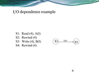
  • 6. 6 I/O dependence example S1: Read (4), A(I) S2: Rewind (4) S3: Write (4), B(I) S4: Rewind (4) S1 S3I/O
  • 7. 7 Control dependence • The order of execution of statements cannot be determined before ru n time o Conditional branches o Successive operations of a looping procedure
  • 8. 8 Control dependence examples Do 20 I = 1, N A(I) = C(I) IF(A(I) .LT. 0) A(I)=1 20 Continue Do 10 I = 1, N IF(A(I-1) .EQ. 0) A(I)=0 10 Continue
  • 9. 9 Resource dependence • Concerned with the conflicts in using shared resources o Integer units o Floating-point units o Registers o Memory areas o ALU o Workplace storage
  • 10. 10 Bernstein’s conditions • Set of conditions for two processes to execute in parallel I1 O2 = Ø I2 O1 = Ø O1 O2 = Ø
  • 11. 11 Bernstein’s Conditions - 2 • In terms of data dependencies, Bernstein’s conditions imply th at two processes can execute in parallel if they are flow-indepe ndent, anti-independent, and output-independent. • The parallelism relation || is commutative (Pi || Pj implies Pj || Pi ), but not transitive (Pi || Pj and Pj || Pk does not imply Pi || Pk ) . Therefore, || is not an equivalence relation. • Intersection of the input sets is allowed.
  • 12. 12 Utilizing Bernstein’s conditions P1 : C = D x E P2 : M = G + C P3 : A = B + C P4 : C = L + M P5 : F = G / E P1 P3 P2 P4 P5
  • 14. 14 Hardware parallelism • A function of cost and performance tradeoffs • Displays the resource utilization patterns of simultan eously executable operations • Denote the number of instruction issues per machin e cycle: k-issue processor • A multiprocessor system with n k-issue processors s hould be able to handle a maximum number of nk th reads of instructions simultaneously
  • 15. 15 Software parallelism • Defined by the control and data dependence of p rograms • A function of algorithm, programming style, and compiler organization • The program flow graph displays the patterns of simultaneously executable operations
  • 16. 16 Mismatch between software and hardware parallelism - 1 L1 L2 L3 L4 X1 X2 + - A B Fig. : Software parallelism Cycle 1 Cycle 2 Cycle 3 Maximum software parallelis m (L=load, X/+/- = arithmeti c) 8 instructions(4 loads and 4 arithmetic operations ) Parallelism varies from 4 to 2 in three cycles
  • 17. 17 Mismatch between software and hardware parall elism - 2 L1 L2 L4 L3X1 X2 + - A B Cycle 1 Cycle 2 Cycle 3 Cycle 4 Cycle 5 Cycle 6 Cycle 7 Same problem, but consid ering the parallelism on a two-issue superscalar pro cessor.
  • 18. 18 Mismatch between software and hardware parall elism - 3 L1 L2 S1 X1 + L5 L3 L4 S2 X2 - L6 BA Cycle 1 Cycle 2 Cycle 3 Cycle 4 Cycle 5 Cycle 6 Same problem, w ith two single-iss ue processors = inserted for s ynchronization Fig. : Dual processor execution
  • 19. 19 Types of Software Parallelism • Control Parallelism – two or more operations can be performed s imultaneously. This can be detected by a compiler, or a programmer can explicitly indicate control parallelism by using special language c onstructs or dividing a program into multiple processes. • Data parallelism – multiple data elements have the same operatio ns applied to them at the same time. This offers the highest potentia l for concurrency (in SIMD and MIMD modes). Synchronization in SIMD machines handled by hardware.
  • 20. 20 Solving the Mismatch Problems • Develop compilation support • Redesign hardware for more efficient exploitation by compilers • Use large register files and sustained instruction pipelining. • Have the compiler fill the branch and load delay slots in code genera ted for RISC processors.
  • 21. 21 The Role of Compilers • Compilers used to exploit hardware features to improve performanc e. • Interaction between compiler and architecture design is a necessity i n modern computer development. • It is not necessarily the case that more software parallelism will impr ove performance in conventional scalar processors. • The hardware and compiler should be designed at the same time.
  • 22. 22 Program Partitioning & Scheduling • The size of the parts or pieces of a program that can be considered fo r parallel execution can vary. • The sizes are roughly classified using the term “granule size,” or sim ply “granularity.” • The simplest measure, for example, is the number of instructions in a program part. • Grain sizes are usually described as fine, medium or coarse, dependi ng on the level of parallelism involved.
  • 23. 23 Latency • Latency is the time required for communication between different s ubsystems in a computer. • Memory latency, for example, is the time required by a processor to access memory. • Synchronization latency is the time required for two processes to sy nchronize their execution. • Computational granularity and communication latency are closely re lated.
  • 24. 24 Levels of Parallelism Jobs or programs Instructions or statements Non-recursive loops or unfolded iterations Procedures, subroutines, tasks, or coroutines Subprograms, job steps or related parts of a program } } Coarse grain Medium grain }Fine grain Increasing com munication dem and and scheduli ng overhead Higher degree of parallelism
  • 25. 25 Instruction Level Parallelism • This fine-grained, or smallest granularity level typically involves less than 20 instructions per grain. The number of candidates for paralle l execution varies from 2 to thousands, with about five instructions o r statements (on the average) being the average level of parallelism. • Advantages: o There are usually many candidates for parallel execution o Compilers can usually do a reasonable job of finding this parallelism
  • 26. 26 Loop-level Parallelism • Typical loop has less than 500 instructions. • If a loop operation is independent between iterations, it can be handl ed by a pipeline, or by a SIMD machine. • Most optimized program construct to execute on a parallel or vector machine • Some loops (e.g. recursive) are difficult to handle. • Loop-level parallelism is still considered fine grain computation.
  • 27. 27 Procedure-level Parallelism • Medium-sized grain; usually less than 2000 instructions. • Detection of parallelism is more difficult than with smaller grains; in terprocedural dependence analysis is difficult and history-sensitive. • Communication requirement less than instruction-level • SPMD (single procedure multiple data) is a special case • Multitasking belongs to this level.
  • 28. 28 Subprogram-level Parallelism • Job step level; grain typically has thousands of instructions; medium - or coarse-grain level. • Job steps can overlap across different jobs. • Multiprograming conducted at this level • No compilers available to exploit medium- or coarse-grain parallelis m at present.
  • 29. 29 Job or Program-Level Parallelism • Corresponds to execution of essentially independent jobs or program s on a parallel computer. • This is practical for a machine with a small number of powerful proc essors, but impractical for a machine with a large number of simple processors (since each processor would take too long to process a sin gle job).
  • 30. 30 Communication Latency • Balancing granularity and latency can yield better performance. • Various latencies attributed to machine architecture, technology, an d communication patterns used. • Latency imposes a limiting factor on machine scalability. Ex. Memo ry latency increases as memory capacity increases, limiting the amou nt of memory that can be used with a given tolerance for communica tion latency.
  • 31. 31 Interprocessor Communication Latency • Needs to be minimized by system designer • Affected by signal delays and communication patterns • Ex. n communicating tasks may require n (n - 1)/2 communication li nks, and the complexity grows quadratically, effectively limiting the number of processors in the system.
  • 32. 32 Grain Packing and Scheduling • Two questions: o How can I partition a program into parallel “pieces” to yield the shorte st execution time? o What is the optimal size of parallel grains? • There is an obvious tradeoff between the time spent scheduling and synchronizing parallel grains and the speedup obtained by paralle l execution. • Solution is both problem-dependent and machine-dependent. • Goal is to produce a short schedule for fast execution of subdivided prog ram modules. • One approach to the problem is called “grain packing”
  • 33. 33 Program Graphs and Packing • A program graph is similar to a dependence graph o Nodes = { (n,s) }, where n = node name, s = size (larger s = larger grain siz e). o Edges = { (v,d) }, where v = variable being “communicated,” and d = com munication delay. • Packing two (or more) nodes produces a node with a larger grain siz e and possibly more edges to other nodes. • Packing is done to eliminate unnecessary communication dela ys or reduce overall scheduling overhead.
  • 35. 35 Scheduling • A schedule is a mapping of nodes to processors and start times such that communication delay requirements are observed, and no two n odes are executing on the same processor at the same time. • Some general scheduling goals o Schedule all fine-grain activities in a node to the same processor to minim ize communication delays. o Select grain sizes for packing to achieve better schedules for a particular p arallel machine.
  • 37. 37 Static multiprocessor scheduling • Grain packing may not be optimal • Dynamic multiprocessor scheduling is an NP-hard problem • Node duplication is a static scheme for multiprocessor scheduling
  • 38. 38 Node duplication • Duplicate some nodes to eliminate idle time and reduce communicat ion delays • Grain packing and node duplication are often used jointly to determi ne the best grain size and corresponding schedule
  • 39. 39 Schedule without node duplication A,4 a,1 b,1 c,8 a,8 c,1 C,1B,1 D,2 E,2 e,4d,4 P1 P2 P2P1 A D B I E C I4 6 13 21 27 23 20 16 14 12 4
  • 40. 40 Schedule with node duplication A,4 a,1 b,1 c,1 a,1 c,1 C’,1B,1 D,2 E,2 P1 P2 P2P1 A D B E C A 4 6 10 14 13 9 6 4 C,1 A’,4 a,1 C 7
  • 41. 41 Grain determination and scheduling optimization Step 1: Construct a fine-grain program graph Step 2: Schedule the fine-grain computation Step 3: Grain packing to produce coarse grains Step 4: Generate a parallel schedule based on the packed graph
  • 42. 42 System Interconnect Architectures • Direct networks for static connections • Indirect networks for dynamic connections • Networks are used for o internal connections in a centralized system among • processors • memory modules • I/O disk arrays o distributed networking of multicomputer nodes
  • 43. 43 Goals and Analysis • The goals of an interconnection network are to provide o low-latency o high data transfer rate o wide communication bandwidth • Analysis includes o latency o bisection bandwidth o data-routing functions o scalability of parallel architecture
  • 44. 44 Network Properties and Routing • Static networks: point-to-point direct connections that will not chan ge during program execution • Dynamic networks: o switched channels dynamically configured to match user program commu nication demands o include buses, crossbar switches, and multistage networks • Both network types also used for inter-PE data routing in SIMD com puters
  • 45. 45 Network Parameters • Network size: The number of nodes (links or channels) in the graph used to represent the network • Node Degree d: The number of edges incident to a node. In the case of unidirectional channels, the number of channels into a node is t he in degree and that out of a node is the out degree. Then the node degree is the sum of the two. • Network Diameter D: The maximum shortest path between any two nodes
  • 46. 46 Network Parameters (cont.) • Bisection Width: o Channel bisection width b: The minimum number of edges (channels) along the cut that divides the network in two equal halves o Each channel has w bit wires o Wire bisection width: B=b*w; B is the wiring density of the network. It provides a good indicator of the max communication bandwidth along the bisection of the network
  • 47. 47 Terminology - 1 • Network usually represented by a graph with a finite nu mber of nodes linked by directed or undirected edges. • Number of nodes in graph = network size . • Number of edges (links or channels) incident on a node = node degree d (also note in and out degrees when edges a re directed). Node degree reflects number of I/O ports as sociated with a node, and should ideally be small and con stant. • Diameter D of a network is the maximum shortest path b etween any two nodes, measured by the number of links t raversed; this should be as small as possible (from a com munication point of view).
  • 48. 48 Terminology - 2 • Channel bisection width b = minimum number of edges cut to split a network into two parts each having the same numb er of nodes. Since each channel has w bit wires, the wire bis ection width B = bw. Bisection width provides good indicati on of maximum communication bandwidth along the bisecti on of a network, and all other cross sections should be boun ded by the bisection width. • Wire (or channel) length = length (e.g. weight) of edges bet ween nodes. • Network is symmetric if the topology is the same looking fro m any node; these are easier to implement or to program. • Other useful characterizing properties: homogeneous nodes ? buffered channels? nodes are switches?
  • 49. 49 Data Routing Functions Data-routing network used for inter-PE data exchange. This network ca n be static (i.e: hypercube) or dynamic (i.e: multistage network) Commonly data-routing functions includes: • Shifting • Rotating • Permutation (one to one) • Broadcast (one to all) • Multicast (many to many) • Personalized broadcast (one to many) • Shuffle • Exchange • Etc.
  • 50. 50 Hypercube Routing Functions • If the vertices of a n-dimensional cube are labeled with n-bit number s so that only one bit differs between each pair of adjacent vertices, t hen n routing functions are defined by the bits in the node (vertex) a ddress. • For example, with a 3-dimensional cube, we can easily identify routi ng functions that exchange data between nodes with addresses that differ in the least significant, most significant, or middle bit. • Figure: 2.15
  • 51. 51 Factors Affecting Network Performance • Functionality – how the network supports data routing, interrupt handling, synchronization, request/message combining, and cohere nce • Network latency – worst-case time for a unit message to be transf erred • Bandwidth – maximum data rate • Hardware complexity – implementation costs for wire, logic, swi tches, connectors, etc. • Scalability – how easily does the scheme adapt to an increasing nu mber of processors, memories, etc.?
  • 52. 52 Static Networks • Linear Array • Ring and Chordal Ring • Barrel Shifter • Tree and Star • Fat Tree • Mesh and Torus
  • 53. 53 Static Networks – Linear Array • N nodes connected by n-1 links (not a bus); segments between differ ent pairs of nodes can be used in parallel. • Internal nodes have degree 2; end nodes have degree 1. • Diameter = n-1 • Bisection = 1 • For small n, this is economical, but for large n, it is obviously inappr opriate.
  • 54. 54 Static Networks – Ring, Chordal Ring • Like a linear array, but the two end nodes are connected by an n th li nk; the ring can be uni- or bi-directional. Diameter is n/2 for a b idirectional ring, or n for a unidirectional ring. • By adding additional links (e.g. “chords” in a circle), the node degree is increased, and we obtain a chordal ring. This reduces the network diameter. • In the limit, we obtain a fully-connected network, with a node degree of n -1 and a diameter of 1.
  • 55. 55 Static Networks – Barrel Shifter • Like a ring, but with additional links between all pairs of nodes that have a distance equal to a power of 2. • With a network of size N = 2n, each node has degree d = 2n -1, and th e network has diameter D = n /2. • Barrel shifter connectivity is greater than any chordal ring of lower n ode degree. • Barrel shifter much less complex than fully-interconnected network.
  • 56. 56
  • 57. 57 Static Networks – Tree and Star • A k-level completely balanced binary tree will have N = 2k – 1 nodes, with maximum node degree of 3 and network diameter is 2(k – 1). • The balanced binary tree is scalable, since it has a constant maximu m node degree. • A star is a two-level tree with a node degree d = N – 1 and a constant diameter of 2.
  • 58. 58 Static Networks – Fat Tree • A fat tree is a tree in which the number of edges between nodes incre ases closer to the root (similar to the way the thickness of limbs incre ases in a real tree as we get closer to the root). • The edges represent communication channels (“wires”), and since co mmunication traffic increases as the root is approached, it seems log ical to increase the number of channels there.
  • 59. 59 Static Networks – Mesh and Torus • Pure mesh – N = n k nodes with links between each adjacent pair of nodes in a row or column (or higher degree). This is not a symmetri c network; interior node degree d = 2k, diameter = k (n – 1). • Illiac mesh (used in Illiac IV computer) – wraparound is allowed, th us reducing the network diameter to about half that of the equivalent pure mesh. • A torus has ring connections in each dimension, and is symmetric. An n n binary torus has node degree of 4 and a diameter of 2 n / 2 .
  • 60. 60 Static Networks – Systolic Array • A systolic array is an arrangement of processing elements and comm unication links designed specifically to match the computation and c ommunication requirements of a specific algorithm (or class of algor ithms). • This specialized character may yield better performance than more g eneralized structures, but also makes them more expensive, and mor e difficult to program.
  • 61. 61 Network Throughput • Network throughput – number of messages a network can handle in a unit time interval. • One way to estimate is to calculate the maximum number of message s that can be present in a network at any instant (its capacity); throu ghput usually is some fraction of its capacity. • A hot spot is a pair of nodes that accounts for a disproportionately la rge portion of the total network traffic (possibly causing congestion). • Hot spot throughput is maximum rate at which messages can be sen t between two specific nodes.
  • 62. 62 Dynamic Connection Networks • Dynamic connection networks can implement all communication pa tterns based on program demands. • In increasing order of cost and performance, these include o bus systems o multistage interconnection networks o crossbar switch networks • Price can be attributed to the cost of wires, switches, arbiters, and co nnectors. • Performance is indicated by network bandwidth, data transfer rate, network latency, and communication patterns supported.
  • 63. 63 Dynamic Networks – Bus Systems • A bus system (contention bus, time-sharing bus) has o a collection of wires and connectors o multiple modules (processors, memories, peripherals, etc.) which con nect to the wires o data transactions between pairs of modules • Bus supports only one transaction at a time. • Bus arbitration logic must deal with conflicting requests. • Lowest cost and bandwidth of all dynamic schemes. • Many bus standards are available.
  • 64. 64 Dynamic Networks – Switch Modules • An a b switch module has a inputs and b outputs. A binary switch has a = b = 2. • It is not necessary for a = b, but usually a = b = 2k, for some integer k . • In general, any input can be connected to one or more of the outputs . However, multiple inputs may not be connected to the same output . • When only one-to-one mappings are allowed, the switch is called a c rossbar switch.
  • 65. 65 Multistage Networks • In general, any multistage network is comprised of a collection of a b switch modules and fixed network modules. The a b s witch modules are used to provide variable permutation or other reordering of the inputs, which are then further reordered by the fixed network modules. • A generic multistage network consists of a sequence alternating dynamic switches (with relatively small values for a and b) with st atic networks (with larger numbers of inputs and outputs). The stati c networks are used to implement interstage connections (ISC).
  • 66. 66 Omega Network • A 2 2 switch can be configured for o Straight-through o Crossover o Upper broadcast (upper input to both outputs) o Lower broadcast (lower input to both outputs) o (No output is a somewhat vacuous possibility as well) • With four stages of eight 2 2 switches, and a static perf ect shuffle for each of the four ISCs, a 16 by 16 Omega net work can be constructed (but not all permutations are po ssible). • In general , an n-input Omega network requires log 2 n st ages of 2 2 switches and n / 2 switch modules.
  • 67. 67
  • 68. 68 Baseline Network • A baseline network can be shown to be topologically equivalent to ot her networks (including Omega), and has a simple recursive generati on procedure. • Stage k (k = 0, 1, …) is an m m switch block (where m = N / 2k ) co mposed entirely of 2 2 switch blocks, each having two configuratio ns: straight through and crossover.
  • 69. 69 4 4 Baseline Network
  • 70. 70 Crossbar Networks • A m n crossbar network can be used to provide a constant latency con nection between devices; it can be thought of as a single stage switch. • Different types of devices can be connected, yielding different constraint s on which switches can be enabled. o With m processors and n memories, one processor may be able to generate request s for multiple memories in sequence; thus several switches might be set in the same row. o For m m interprocessor communication, each PE is connected to both an input a nd an output of the crossbar; only one switch in each row and column can be turne d on simultaneously. Additional control processors are used to manage the crossba r itself.