SlideShare a Scribd company logo
Overview of Machine Learning Raymond J. Mooney Department of Computer Sciences University of Texas at Austin
What is Learning? Definition by H. Simon: “Any process by which a system improves performance.” What is the task? Classification/categorization Problem solving Planning Control Language understanding
Classification Examples Medical diagnosis Credit card applications or transactions DNA sequences  Promoter Splice-junction Protein structure Spoken words Handwritten characters Astronomical images Market basket analysis
Other Tasks Solving calculus problems Playing games Checkers Chess Backgammon Pole balancing Driving a car Flying a helicopter Robot navigation
How is Performance Measured? Classification accuracy False positives False negatives Precision/Recall/F-measure Solution correctness and quality (optimality) Number of questions answered correctly Distance traveled for navigation problem Percentage of games won against an opponent Time to find a solution
Training Experience Direct supervision Checkers board positions labeled with correct move. Road images with correct steering position. Indirect supervision (delayed reward, reinforcement learning) Choose sequence of checkers move and eventually win or lose game. Drive car and rewarded if reach destination.
Types of Direct Supervision Examples chosen by a benevolent teacher Near miss negative examples Random examples from the environment. Positive and negative examples Positive examples only Choose examples for a teacher (oracle) to classify. Design and run one’s own experiments.
Categorization Given: A description of an instance,  x  X , where X is the  instance language  or  instance space . A fixed set of categories:  C= { c 1 ,  c 2 ,… c n } A categorization function,  c ( x ), whose domain is  X  and whose range is  C . Determine: The category of  x :  c ( x )  C,
Learning for Categorization A training example is an instance  x  X,  paired with its correct category  c ( x ): < x ,  c ( x )> for an unknown categorization function,  c .  Given: A set of training examples,  D . An hypothesis space,  H , of possible categorization functions,  h ( x ). Find a consistent hypothesis,  h ( x )  H , such that:
Sample Category Learning Problem Instance language: <size, color, shape> size    {small, medium, large} color    {red, blue, green} shape    {square, circle, triangle} C  = {positive, negative} D : negative triangle red small 3 positive circle red large 2 positive circle red small 1 negative circle blue large 4 Category Shape Color Size Example
General Learning Issues Many hypotheses are usually consistent with the training data. Bias Any criteria other than consistency with the training data that is used to select a hypothesis. Classification accuracy (% of instances classified correctly). Measured on independent test data. Training time (efficiency of training algorithm). Testing time (efficiency of subsequent classification).
Learning as Search Learning for categorization requires searching for a consistent hypothesis in a given space,  H . Enumerate and test is a possible algorithm for any finite or countably infinite  H. Most hypothesis spaces are very large: Conjunctions on  n  binary features: 3 n   All binary functions on  n  binary features: 2 Efficient algorithms needed for finding a consistent hypothesis without enumerating them all. 2 n
Types of Bias Language Bias : Limit hypothesis space  a priori  to a restricted set of functions. Search Bias : Employ a hypothesis space that includes all possible functions but use a search algorithm that prefers simpler hypotheses. Since finding the simplest hypothesis is usually intractable (e.g. NP-Hard), satisficing heuristic search is usually employed.
Generalization Hypotheses must generalize to correctly classify instances not in the training data. Simply memorizing training examples is a consistent hypothesis that does not generalize. Occam’s razor : Finding a  simple  hypothesis helps ensure generalization.
Over-Fitting Frequently, complete consistency with the training data is not desirable. A completely consistent hypothesis may be fitting errors and noise in the training data, preventing generalization. There is usually a trade-off between hypothesis complexity and degree of fit to the training data. Methods for preventing over-fitting: Predetermined strong language bias. “ Pruning” or “early stopping” criteria to prevent learning overly-complex hypotheses.
Learning Approaches EM (inside-outside) PCFG Probabilistic Grammar EM (forward-backward) HMM Hidden Markov Model Maximum likelihood/EM Bayesian Network Bayes Net Memorize then Find closest match Stored instances Nearest Neighbor Instance/Case-based Gradient descent Artificial neural net Neural Network Greedy divide & conquer Decision trees Decision tree induction Greedy set covering Rules Rule Induction Search Method Representation Approach
More Learning Approaches Genetic algorithm Rules/neural-nets Evolutionary computation Greedy set covering Prolog program Inductive Logic Programming Averaging Average instance Prototype Quadratic optimization Hyperplane Support Vector Machine (SVM) Generalized/Improved Iterative Scaling Exponential Model Maximum Entropy (MaxEnt) Search Method Representation Approach
Text Categorization Assigning documents to a fixed set of categories. Applications: Web pages  Recommending Yahoo-like classification Newsgroup Messages  Recommending spam filtering News articles  Personalized newspaper Email messages  Routing Prioritizing  Folderizing spam filtering
Relevance Feedback Architecture Rankings IR System Document corpus Ranked Documents 1. Doc1  2. Doc2  3. Doc3  . . 1. Doc1   2. Doc2   3. Doc3   . . Feedback Query String Revised Query ReRanked Documents 1. Doc2  2. Doc4  3. Doc5  . . Query Reformulation
Using Relevance Feedback (Rocchio) Relevance feedback methods can be adapted for text categorization. Use standard TF/IDF weighted vectors to represent text documents (normalized by maximum term frequency). For each category, compute a  prototype  vector by summing the vectors of the training documents in the category. Assign test documents to the category with the closest prototype vector based on cosine similarity.
Illustration of Rocchio Text Categorization
Rocchio Text Categorization Algorithm (Training) Assume the set of categories is { c 1 ,  c 2 ,… c n } For  i  from 1 to  n  let  p i  = <0, 0,…,0>  ( init. prototype vectors ) For each training example < x ,  c ( x )>     D Let  d  be the frequency normalized TF/IDF term vector for doc  x Let  i  =  j : ( c j  =  c ( x )) ( sum all the document vectors in c i  to get  p i ) Let  p i  =  p i  +  d
Rocchio Text Categorization Algorithm (Test) Given test document  x Let  d  be the TF/IDF weighted term vector for  x Let  m  =  –2  ( init.   maximum cosSim ) For  i  from 1 to  n : ( compute similarity to prototype vector ) Let  s  = cosSim( d ,  p i ) if  s  >  m let  m  =  s let  r = c i  ( update most similar class prototype ) Return class  r
Rocchio Properties  Does not guarantee a consistent hypothesis. Forms a simple generalization of the examples in each class (a  prototype ). Prototype vector does not need to be averaged or otherwise normalized for length since cosine similarity is insensitive to vector length. Classification is based on similarity to class prototypes.
Rocchio Time Complexity Note:  The time to add two sparse vectors is proportional to minimum number of non-zero entries in the two vectors. Training Time :  O(| D |( L d  + | V d |)) = O(| D |  L d )  where  L d  is the average length of a document in  D  and  V d  is the average vocabulary size for a document in  D. Test Time : O( L t  + |C||V t | )  where  L t  is the average length of a test document and | V t  |  is the average vocabulary size for a test document. Assumes lengths of  p i  vectors are computed and stored during training, allowing cosSim( d ,  p i ) to be computed  in time proportional to the number of non-zero entries in  d  (i.e.  |V t | )
Nearest-Neighbor Learning Algorithm Learning is just storing the representations of the training examples in  D . Testing instance  x : Compute similarity between  x  and all examples in  D . Assign  x  the category of the most similar example in  D . Does not explicitly compute a generalization or category prototypes. Also called: Case-based Instance-based Memory-based Lazy learning
K Nearest-Neighbor Using only the closest example to determine categorization is subject to errors due to: A single atypical example.  Noise (i.e. error) in the category label of a single training example. More robust alternative is to find the  k  most-similar examples and return the majority category of these  k  examples. Value of  k  is typically odd to avoid ties, 3 and 5 are most common.
Similarity Metrics Nearest neighbor method depends on a similarity (or distance) metric. Simplest for continuous  m -dimensional instance space is  Euclidian distance . Simplest for  m -dimensional binary instance space is  Hamming distance  (number of feature values that differ). For text, cosine similarity of TF-IDF weighted vectors is typically most effective.
3 Nearest Neighbor Illustration (Euclidian Distance) . . . . . . . . . . .
K Nearest Neighbor for Text Training: For each each   training example < x ,  c ( x )>     D Compute the corresponding TF-IDF vector,  d x , for document  x Test instance  y : Compute TF-IDF vector  d  for document  y For each  < x ,  c ( x )>     D Let  s x  = cosSim( d ,  d x ) Sort examples,  x , in  D  by decreasing value of  s x Let  N  be the first  k  examples in D.  ( get most similar neighbors ) Return the majority class of examples in  N
Illustration of 3 Nearest Neighbor for Text
Rocchio Anomoly  Prototype models have problems with polymorphic (disjunctive) categories.
3 Nearest Neighbor Comparison Nearest Neighbor tends to handle polymorphic categories better.
Nearest Neighbor Time Complexity Training Time : O(| D |  L d ) to compose  TF-IDF vectors. Testing Time : O( L t  + |D||V t | ) to compare to all training vectors. Assumes lengths of  d x   vectors are computed and stored during training, allowing cosSim( d ,  d x ) to be computed  in time proportional to the number of non-zero entries in  d  (i.e.  |V t | )   Testing time can be high for large training sets.
Nearest Neighbor with Inverted Index Determining  k  nearest neighbors is the same as determining the  k  best retrievals using the test document as a query to a database of training documents. Use standard VSR inverted index methods to find the  k  nearest neighbors. Testing Time : O( B|V t | )  where  B  is the average number of training documents in which a test-document word appears. Therefore, overall classification is O( L t  + B|V t | )  Typically  B  << | D |
Bayesian Methods Learning and classification methods based on probability theory. Bayes theorem plays a critical role in probabilistic learning and classification. Uses  prior  probability of each category given no information about an item. Categorization produces a  posterior  probability distribution over the possible categories given a description of an item.
Conditional Probability  P( A  |  B ) is the probability of  A  given  B Assumes that  B  is all and only information known. Defined by: A B
Independence A  and  B  are  independent  iff: Therefore, if  A  and  B  are independent: These two constraints are logically equivalent
Bayes Theorem Simple proof from definition of conditional probability: QED: (Def. cond. prob.) (Def. cond. prob.)
Bayesian Categorization Let   set of categories be { c 1 ,  c 2 ,… c n } Let  E  be description of an instance. Determine category of  E  by determining for each  c i P( E ) can be determined since categories are complete and disjoint.
Bayesian Categorization (cont.) Need to know: Priors: P( c i )  Conditionals: P( E  |  c i ) P( c i ) are easily estimated from data.  If  n i  of the examples in  D  are in  c i , then  P( c i ) =  n i  / | D| Assume instance is a conjunction of binary features: Too many possible instances (exponential in  m ) to estimate all P( E  |  c i )
Naïve Bayesian Categorization If we assume features of an instance are independent given the category ( c i ) ( conditionally independent ). Therefore, we then only need to know  P( e j  |  c i ) for each feature and category.
Naïve Bayes Example C = {allergy, cold, well} e 1  = sneeze;  e 2  = cough;  e 3  = fever E = {sneeze, cough,   fever} 0.4 0.7 0.01 P(fever| c i ) 0.7 0.8 0.1 P(cough| c i ) 0.9 0.9 0.1 P(sneeze| c i ) 0.05 0.05 0.9 P( c i ) Allergy Cold Well Prob
Naïve Bayes Example (cont.) P(well | E) = (0.9)(0.1)(0.1)(0.99)/P(E)=0.0089/P(E) P(cold | E) = (0.05)(0.9)(0.8)(0.3)/P(E)=0.01/P(E) P(allergy | E) = (0.05)(0.9)(0.7)(0.6)/P(E)=0.019/P(E) Most probable category: allergy P(E) = 0.0089 + 0.01 + 0.019 = 0.0379 P(well | E) = 0.23 P(cold | E) = 0.26 P(allergy | E) = 0.50 E={sneeze, cough,   fever} 0.4 0.7 0.01 P(fever |  c i ) 0.7 0.8 0.1 P(cough |  c i ) 0.9 0.9 0.1 P(sneeze |  c i ) 0.05 0.05 0.9 P( c i ) Allergy Cold Well Probability
Estimating Probabilities Normally, probabilities are estimated based on observed frequencies in the training data. If  D  contains  n i   examples in category  c i , and  n ij  of these  n i  examples contains feature  e j , then: However, estimating such probabilities from small training sets is error-prone. If due only to chance, a rare feature,  e k , is always false in the training data,   c i  :P( e k  |  c i ) = 0. If  e k  then occurs in a test example,  E , the result is that   c i : P( E  |  c i ) = 0 and   c i : P( c i  |  E ) = 0
Smoothing To account for estimation from small samples, probability estimates are adjusted or  smoothed . Laplace smoothing using an  m -estimate assumes that each feature is given a prior probability,  p , that is assumed to have been previously observed in a “virtual” sample of size  m . For binary features,  p  is simply assumed to be 0.5.
Naïve Bayes for Text Modeled as generating a bag of words for a document in a given category by repeatedly sampling with replacement from a vocabulary  V  =  { w 1 ,  w 2 ,… w m }  based on the probabilities P( w j   |  c i ). Smooth probability estimates with Laplace  m -estimates assuming a uniform distribution over all words ( p  = 1/| V |) and  m  = | V | Equivalent to a virtual sample of seeing each word in each category exactly once.
Text Naïve Bayes Algorithm (Train) Let  V  be the vocabulary of all words in the documents in  D For each category  c i     C Let  D i   be the subset of documents in  D  in category  c i P( c i ) = | D i | / | D | Let  T i  be the concatenation of all the documents in  D i Let  n i  be the total number of word occurrences in  T i For each word  w j     V Let  n ij  be the number of occurrences of  w j  in  T i Let P( w i   |  c i ) = ( n ij  + 1) / ( n i  + | V |)
Text Naïve Bayes Algorithm (Test) Given a test document  X Let  n  be the number of word occurrences in  X Return the category: where  a j  is the word occurring the  j th position in  X
Naïve Bayes Time Complexity Training Time :  O(| D | L d  + | C || V |))  where  L d  is the average length of a document in  D. Assumes  V  and all  D i  ,  n i , and  n ij  pre-computed in O(| D | L d ) time during one pass through all of the data. Generally just O(| D | L d ) since usually | C || V | < | D | L d   Test Time : O( |C| L t )  where  L t  is the average length of a test document. Very efficient overall, linearly proportional to the time needed to just read in all the data. Similar to Rocchio time complexity.
Underflow Prevention Multiplying lots of probabilities, which are between 0 and 1 by definition, can result in floating-point underflow. Since log( xy ) = log( x ) + log( y ), it is better to perform all computations by summing logs of probabilities rather than multiplying probabilities. Class with highest final un-normalized log probability score is still the most probable.
Naïve Bayes Posterior Probabilities Classification results of naïve Bayes (the class with maximum posterior probability) are usually fairly accurate. However, due to the inadequacy of the conditional independence assumption, the actual posterior-probability numerical estimates are not. Output probabilities are generally very close to 0 or 1.
Evaluating Categorization Evaluation must be done on test data that are independent of the training data (usually a disjoint set of instances). Classification accuracy :  c / n  where  n  is the total number of test instances and  c  is the number of test instances correctly classified by the system. Results can vary based on sampling error due to different training and test sets. Average results over multiple training and test sets (splits of the overall data) for the best results.
N -Fold Cross-Validation Ideally, test and training sets are independent on each trial. But this would require too much labeled data. Partition data into  N  equal-sized disjoint segments. Run  N  trials, each time using a different segment of the data for testing, and training on the remaining  N  1 segments. This way, at least test-sets are independent. Report average classification accuracy over the  N  trials. Typically,  N  = 10.
Learning Curves In practice, labeled data is usually rare and expensive. Would like to know how performance varies with the number of training instances. Learning curves  plot classification accuracy on independent test data ( Y  axis) versus number of training examples ( X  axis).
N -Fold Learning Curves Want learning curves averaged over multiple trials. Use  N -fold cross validation to generate  N  full training and test sets. For each trial, train on increasing fractions of the training set, measuring accuracy on the test data for each point on the desired learning curve.
Sample Document Corpus 600 science pages from the web. 200 random samples each from the Yahoo indices for biology, physics, and chemistry.
Sample Learning Curve (Yahoo Science Data)
Clustering Partition unlabeled examples into disjoint subsets of  clusters , such that: Examples within a cluster are very similar Examples in different clusters are very different Discover new categories in an  unsupervised  manner (no sample category labels provided).
Clustering Example . . . . . . . . . . . . . . . . . . . . . . . . . . . . . . . .
Hierarchical Clustering Build a tree-based hierarchical taxonomy ( dendrogram ) from a set of unlabeled examples. Recursive application of a standard clustering algorithm can produce a hierarchical clustering. animal vertebrate fish reptile amphib. mammal  worm insect crustacean invertebrate
Aglommerative vs. Divisive Clustering Aglommerative  ( bottom-up ) methods start with each example in its own cluster and iteratively combine them to form larger and larger clusters. Divisive  ( partitional, top-down ) separate all examples immediately into clusters.
Direct Clustering Method Direct clustering  methods require a specification of the number of clusters,  k , desired. A  clustering evaluation   function   assigns a real-value quality measure to a clustering. The number of clusters can be determined automatically by explicitly generating clusterings for multiple values of  k  and choosing the best result according to a clustering evaluation function.
Hierarchical Agglomerative Clustering  (HAC) Assumes a  similarity function  for determining the similarity of two instances. Starts with all instances in a separate cluster and then repeatedly joins the two clusters that are most similar until there is only one cluster. The history of merging forms a binary tree or hierarchy.
HAC Algorithm Start with all instances in their own cluster. Until there is only one cluster: Among the current clusters, determine the two  clusters,  c i  and  c j , that are most similar. Replace  c i  and  c j  with a single cluster  c i     c j
Cluster Similarity Assume a similarity function that determines the similarity of two instances:  sim ( x , y ). Cosine similarity of document vectors. How to compute similarity of two clusters each possibly containing multiple instances? Single Link : Similarity of two most similar members. Complete Link : Similarity of two least similar members. Group Average : Average similarity between members.
Single Link Agglomerative Clustering Use maximum similarity of pairs: Can result in “straggly” (long and thin) clusters due to  chaining effect . Appropriate in some domains, such as clustering islands.
Single Link Example
Complete Link Agglomerative Clustering Use minimum similarity of pairs: Makes more “tight,” spherical clusters that are typically preferable.
Complete Link Example
Computational Complexity In the first iteration, all HAC methods need to compute similarity of all pairs of  n  individual instances which is O( n 2 ). In each of the subsequent  n  2 merging iterations, it must compute the distance between the most recently created cluster and all other existing clusters. In order to maintain an overall O( n 2 ) performance, computing similarity to each other cluster must be done in constant time.
Computing Cluster Similarity After merging  c i  and  c j , the similarity of the resulting cluster to any other cluster,  c k , can be computed by: Single Link: Complete Link:
Group Average Agglomerative Clustering Use average similarity across all pairs within the merged cluster to measure the similarity of two clusters. Compromise between single and complete link. Averaged across all ordered pairs in the merged cluster instead of unordered pairs  between  the two clusters.
Computing Group Average Similarity Assume cosine similarity and normalized vectors with unit length. Always maintain sum of vectors in each cluster. Compute similarity of clusters in constant time:
Non-Hierarchical Clustering Typically must provide the number of desired clusters,  k . Randomly choose  k  instances as  seeds , one per cluster.  Form initial clusters based on these seeds. Iterate, repeatedly reallocating instances to different clusters to improve the overall clustering. Stop when clustering converges or after a fixed number of iterations.
K-Means Assumes instances are real-valued vectors. Clusters based on  centroids ,  center of gravity , or mean of points in a cluster,  c : Reassignment of instances to clusters is based on distance to the current cluster centroids.
Distance Metrics Euclidian distance (L 2  norm): L 1  norm: Cosine Similarity (transform to a distance by subtracting from 1):
K-Means Algorithm Let  d  be the distance measure between instances. Select  k  random instances { s 1 ,  s 2 ,…  s k } as seeds. Until clustering converges or other stopping criterion: For each instance  x i : Assign  x i  to the cluster  c j   such that  d ( x i ,  s j ) is minimal. ( Update the seeds to the centroid of each cluster ) For each cluster  c j s j  =   ( c j )
K Means Example (K=2) Reassign clusters Converged! Pick seeds Reassign clusters Compute centroids x x Reasssign clusters x x x x Compute centroids
Time Complexity Assume computing distance between two instances is O( m ) where  m  is the dimensionality of the vectors. Reassigning clusters: O( kn ) distance computations, or O( knm ). Computing centroids: Each instance vector gets added once to some centroid: O( nm ). Assume these two steps are each done once for  I  iterations:  O( Iknm ). Linear in all relevant factors, assuming a fixed number of iterations, more efficient than O(n 2 ) HAC.
Seed Choice Results can vary based on random seed selection. Some seeds can result in poor convergence rate, or convergence to sub-optimal clusterings. Select good seeds using a heuristic or the results of another method.
Buckshot Algorithm Combines HAC and K-Means clustering. First randomly take a sample of instances of size   n   Run group-average HAC on this sample, which takes only O( n ) time. Use the results of HAC as initial seeds for K-means. Overall algorithm is O( n ) and avoids problems of bad seed selection.
Text Clustering HAC and K-Means have been applied to text in a straightforward way. Typically use  normalized , TF/IDF-weighted vectors and cosine similarity. Optimize computations for sparse vectors. Applications: During retrieval, add other documents in the same cluster as the initial retrieved documents to improve recall. Clustering of results of retrieval to present more organized results to the user ( à  la Northernlight folders). Automated production of hierarchical taxonomies of documents for browsing purposes ( à  la Yahoo & DMOZ).
Soft Clustering Clustering typically assumes that each instance is given a “hard” assignment to exactly one cluster. Does not allow uncertainty in class membership or for an instance to belong to more than one cluster. Soft clustering  gives probabilities that an instance belongs to each of a set of clusters. Each instance is assigned a probability distribution across a set of discovered categories (probabilities of all categories must sum to 1).
Expectation Maximization (EM) Probabilistic method for soft clustering. Direct method that assumes  k  clusters: { c 1 ,  c 2 ,…  c k }  Soft version of  k -means. Assumes a probabilistic model of categories that allows computing P( c i  |  E )   for each category,  c i , for a given example,  E . For text, typically assume a naïve-Bayes category model. Parameters    = {P( c i ), P( w j  |  c i ):  i  {1,… k },  j    {1,…,| V |}}
EM Algorithm Iterative method for learning probabilistic categorization model from unsupervised data. Initially assume random assignment of examples to categories. Learn an initial probabilistic model by estimating model parameters    from this randomly labeled data. Iterate following two steps until convergence: Expectation (E-step):  Compute P( c i  |  E )   for each example given the current model, and probabilistically re-label the examples based on these posterior probability estimates. Maximization (M-step):  Re-estimate the model parameters,   , from the probabilistically re-labeled data.
Learning from Probabilistically Labeled Data  Instead of training data labeled with “hard” category labels, training data is labeled with “soft” probabilistic category labels. When estimating model parameters    from training data, weight counts by the corresponding probability of the given category label. For example, if P( c 1  |  E ) = 0.8 and P( c 2  |  E ) = 0.2,  each word  w j  in  E  contributes only 0.8 towards the counts  n 1  and  n 1 j , and 0.2 towards the counts  n 2  and  n 2 j .
Naïve Bayes EM Randomly assign examples probabilistic category labels. Use standard naïve-Bayes training to learn a probabilistic model  with parameters    from the labeled data. Until convergence or until maximum number of iterations reached: E-Step : Use the naïve Bayes model     to compute P( c i  |  E ) for each category and example, and re-label each example  using these probability values as soft category labels. M-Step : Use standard naïve-Bayes training to re-estimate the  parameters    using these new probabilistic category labels.
Semi-Supervised Learning For supervised categorization, generating labeled training data is expensive. Idea : Use unlabeled data to aid supervised categorization. Use EM in a  semi-supervised  mode by training EM on both labeled and unlabeled data. Train initial probabilistic model on user-labeled subset of data instead of randomly labeled unsupervised data.  Labels of user-labeled examples are “frozen” and never relabeled during EM iterations. Labels of unsupervised data are constantly probabilistically relabeled by EM.
Semi-Supervised Example Assume “quantum” is present in several labeled physics documents, but “Heisenberg” occurs in  none  of the  labeled  data. From labeled data, learn that “quantum” is indicative of a physics document. When labeling unsupervised data, label several documents with “quantum”  and  “Heisenberg” correctly with the “physics” category. When retraining, learn that “Heisenberg” is also indicative of a physics document. Final learned model is able to correctly assign documents containing  only  “Heisenberg” to physics.
Semi-Supervision Results Experiments on assigning messages from 20 Usenet newsgroups their proper newsgroup label. With very few labeled examples (2 examples per class), semi-supervised EM improved accuracy from 27% (supervised data only) to 43% (supervised + unsupervised data). With more labeled examples, semi-supervision can actually decrease accuracy, but refinements to standard EM can prevent this. For semi-supervised EM to work, the “natural clustering of data” must be consistent with the desired categories.
Active Learning Select only the most informative examples for labeling. Initial methods: Uncertainty sampling Committee-based sampling Error-reduction sampling
Weak Supervision Sometimes uncertain labeling can be inferred. Learning apprentices Inferred feedback Click patterns, reading time, non-verbal cues Delayed feedback Reinforcement learning Programming by Demonstration
Prior Knowledge Use of prior declarative knowledge in learning. Initial methods: Explanation-based Learning Theory Refinement Bayesian Priors Reinforcement Learning with Advice
Learning to Learn Many applications require learning for  multiple, related  problems. What can be learned from one problem that can aid the learning for other problems? Initial approaches: Multi-task learning Life-long learning Learning similarity metrics Supra-classifiers

More Related Content

What's hot (19)

PDF
17 Machine Learning Radial Basis Functions
Andres Mendez-Vazquez
 
PPT
20070702 Text Categorization
midi
 
PDF
A Study of Efficiency Improvements Technique for K-Means Algorithm
IRJET Journal
 
PDF
Mini-batch Variational Inference for Time-Aware Topic Modeling
Tomonari Masada
 
PDF
Latent Semantic Word Sense Disambiguation Using Global Co-Occurrence Information
csandit
 
PDF
Density Based Clustering
SSA KPI
 
PDF
Performance Analysis of Different Clustering Algorithm
IOSR Journals
 
PPTX
Recommendation system
Ding Li
 
PDF
PSF_Introduction_to_R_Package_for_Pattern_Sequence (1)
neeraj7svp
 
PDF
A Novel Approach to Mathematical Concepts in Data Mining
ijdmtaiir
 
PPT
3.4 density and grid methods
Krish_ver2
 
PDF
Deep learning ensembles loss landscape
Devansh16
 
PPTX
Selection K in K-means Clustering
Junghoon Kim
 
PPTX
Analytical learning
swapnac12
 
PPTX
Inductive analytical approaches to learning
swapnac12
 
PPT
2.7 other classifiers
Krish_ver2
 
PDF
Enhanced Genetic Algorithm with K-Means for the Clustering Problem
Anders Viken
 
PDF
ANN Based POS Tagging For Nepali Text
ijnlc
 
PDF
10 clusbasic
JoonyoungJayGwak
 
17 Machine Learning Radial Basis Functions
Andres Mendez-Vazquez
 
20070702 Text Categorization
midi
 
A Study of Efficiency Improvements Technique for K-Means Algorithm
IRJET Journal
 
Mini-batch Variational Inference for Time-Aware Topic Modeling
Tomonari Masada
 
Latent Semantic Word Sense Disambiguation Using Global Co-Occurrence Information
csandit
 
Density Based Clustering
SSA KPI
 
Performance Analysis of Different Clustering Algorithm
IOSR Journals
 
Recommendation system
Ding Li
 
PSF_Introduction_to_R_Package_for_Pattern_Sequence (1)
neeraj7svp
 
A Novel Approach to Mathematical Concepts in Data Mining
ijdmtaiir
 
3.4 density and grid methods
Krish_ver2
 
Deep learning ensembles loss landscape
Devansh16
 
Selection K in K-means Clustering
Junghoon Kim
 
Analytical learning
swapnac12
 
Inductive analytical approaches to learning
swapnac12
 
2.7 other classifiers
Krish_ver2
 
Enhanced Genetic Algorithm with K-Means for the Clustering Problem
Anders Viken
 
ANN Based POS Tagging For Nepali Text
ijnlc
 
10 clusbasic
JoonyoungJayGwak
 

Similar to lecture_mooney.ppt (20)

PPT
LECTURE8.PPT
butest
 
PPT
Machine Learning
butest
 
PDF
A Few Useful Things to Know about Machine Learning
nep_test_account
 
DOC
learningIntro.doc
butest
 
DOC
learningIntro.doc
butest
 
PPT
Download presentation source
butest
 
PPTX
Introduction
butest
 
PPTX
Introduction
butest
 
PPTX
Introduction
butest
 
PPT
Machine Learning: Decision Trees Chapter 18.1-18.3
butest
 
PPT
ML_Overview.ppt
ParveshKumar17303
 
PPTX
ML_Overview.pptx
ssuserb0b8ed1
 
PPT
ML_Overview.ppt
vijay251387
 
PPT
ML overview
NoopurRathore1
 
PPT
Machine Learning and Inductive Inference
butest
 
PPT
coppin chapter 10e.ppt
butest
 
PPT
Introduction to Machine Learning.
butest
 
PPT
c23_ml1.ppt
Faiz430036
 
PPT
Data.Mining.C.6(II).classification and prediction
Margaret Wang
 
PPT
classification of learning methods...ppt
GeethaPanneer
 
LECTURE8.PPT
butest
 
Machine Learning
butest
 
A Few Useful Things to Know about Machine Learning
nep_test_account
 
learningIntro.doc
butest
 
learningIntro.doc
butest
 
Download presentation source
butest
 
Introduction
butest
 
Introduction
butest
 
Introduction
butest
 
Machine Learning: Decision Trees Chapter 18.1-18.3
butest
 
ML_Overview.ppt
ParveshKumar17303
 
ML_Overview.pptx
ssuserb0b8ed1
 
ML_Overview.ppt
vijay251387
 
ML overview
NoopurRathore1
 
Machine Learning and Inductive Inference
butest
 
coppin chapter 10e.ppt
butest
 
Introduction to Machine Learning.
butest
 
c23_ml1.ppt
Faiz430036
 
Data.Mining.C.6(II).classification and prediction
Margaret Wang
 
classification of learning methods...ppt
GeethaPanneer
 
Ad

More from butest (20)

PDF
EL MODELO DE NEGOCIO DE YOUTUBE
butest
 
DOC
1. MPEG I.B.P frame之不同
butest
 
PDF
LESSONS FROM THE MICHAEL JACKSON TRIAL
butest
 
PPT
Timeline: The Life of Michael Jackson
butest
 
DOCX
Popular Reading Last Updated April 1, 2010 Adams, Lorraine The ...
butest
 
PDF
LESSONS FROM THE MICHAEL JACKSON TRIAL
butest
 
PPTX
Com 380, Summer II
butest
 
PPT
PPT
butest
 
DOCX
The MYnstrel Free Press Volume 2: Economic Struggles, Meet Jazz
butest
 
DOC
MICHAEL JACKSON.doc
butest
 
PPTX
Social Networks: Twitter Facebook SL - Slide 1
butest
 
PPT
Facebook
butest
 
DOCX
Executive Summary Hare Chevrolet is a General Motors dealership ...
butest
 
DOC
Welcome to the Dougherty County Public Library's Facebook and ...
butest
 
DOC
NEWS ANNOUNCEMENT
butest
 
DOC
C-2100 Ultra Zoom.doc
butest
 
DOC
MAC Printing on ITS Printers.doc.doc
butest
 
DOC
Mac OS X Guide.doc
butest
 
DOC
hier
butest
 
DOC
WEB DESIGN!
butest
 
EL MODELO DE NEGOCIO DE YOUTUBE
butest
 
1. MPEG I.B.P frame之不同
butest
 
LESSONS FROM THE MICHAEL JACKSON TRIAL
butest
 
Timeline: The Life of Michael Jackson
butest
 
Popular Reading Last Updated April 1, 2010 Adams, Lorraine The ...
butest
 
LESSONS FROM THE MICHAEL JACKSON TRIAL
butest
 
Com 380, Summer II
butest
 
PPT
butest
 
The MYnstrel Free Press Volume 2: Economic Struggles, Meet Jazz
butest
 
MICHAEL JACKSON.doc
butest
 
Social Networks: Twitter Facebook SL - Slide 1
butest
 
Facebook
butest
 
Executive Summary Hare Chevrolet is a General Motors dealership ...
butest
 
Welcome to the Dougherty County Public Library's Facebook and ...
butest
 
NEWS ANNOUNCEMENT
butest
 
C-2100 Ultra Zoom.doc
butest
 
MAC Printing on ITS Printers.doc.doc
butest
 
Mac OS X Guide.doc
butest
 
hier
butest
 
WEB DESIGN!
butest
 
Ad

lecture_mooney.ppt

  • 1. Overview of Machine Learning Raymond J. Mooney Department of Computer Sciences University of Texas at Austin
  • 2. What is Learning? Definition by H. Simon: “Any process by which a system improves performance.” What is the task? Classification/categorization Problem solving Planning Control Language understanding
  • 3. Classification Examples Medical diagnosis Credit card applications or transactions DNA sequences Promoter Splice-junction Protein structure Spoken words Handwritten characters Astronomical images Market basket analysis
  • 4. Other Tasks Solving calculus problems Playing games Checkers Chess Backgammon Pole balancing Driving a car Flying a helicopter Robot navigation
  • 5. How is Performance Measured? Classification accuracy False positives False negatives Precision/Recall/F-measure Solution correctness and quality (optimality) Number of questions answered correctly Distance traveled for navigation problem Percentage of games won against an opponent Time to find a solution
  • 6. Training Experience Direct supervision Checkers board positions labeled with correct move. Road images with correct steering position. Indirect supervision (delayed reward, reinforcement learning) Choose sequence of checkers move and eventually win or lose game. Drive car and rewarded if reach destination.
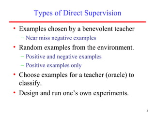
  • 7. Types of Direct Supervision Examples chosen by a benevolent teacher Near miss negative examples Random examples from the environment. Positive and negative examples Positive examples only Choose examples for a teacher (oracle) to classify. Design and run one’s own experiments.
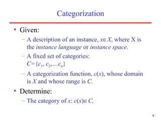
  • 8. Categorization Given: A description of an instance, x  X , where X is the instance language or instance space . A fixed set of categories: C= { c 1 , c 2 ,… c n } A categorization function, c ( x ), whose domain is X and whose range is C . Determine: The category of x : c ( x )  C,
  • 9. Learning for Categorization A training example is an instance x  X, paired with its correct category c ( x ): < x , c ( x )> for an unknown categorization function, c . Given: A set of training examples, D . An hypothesis space, H , of possible categorization functions, h ( x ). Find a consistent hypothesis, h ( x )  H , such that:
  • 10. Sample Category Learning Problem Instance language: <size, color, shape> size  {small, medium, large} color  {red, blue, green} shape  {square, circle, triangle} C = {positive, negative} D : negative triangle red small 3 positive circle red large 2 positive circle red small 1 negative circle blue large 4 Category Shape Color Size Example
  • 11. General Learning Issues Many hypotheses are usually consistent with the training data. Bias Any criteria other than consistency with the training data that is used to select a hypothesis. Classification accuracy (% of instances classified correctly). Measured on independent test data. Training time (efficiency of training algorithm). Testing time (efficiency of subsequent classification).
  • 12. Learning as Search Learning for categorization requires searching for a consistent hypothesis in a given space, H . Enumerate and test is a possible algorithm for any finite or countably infinite H. Most hypothesis spaces are very large: Conjunctions on n binary features: 3 n All binary functions on n binary features: 2 Efficient algorithms needed for finding a consistent hypothesis without enumerating them all. 2 n
  • 13. Types of Bias Language Bias : Limit hypothesis space a priori to a restricted set of functions. Search Bias : Employ a hypothesis space that includes all possible functions but use a search algorithm that prefers simpler hypotheses. Since finding the simplest hypothesis is usually intractable (e.g. NP-Hard), satisficing heuristic search is usually employed.
  • 14. Generalization Hypotheses must generalize to correctly classify instances not in the training data. Simply memorizing training examples is a consistent hypothesis that does not generalize. Occam’s razor : Finding a simple hypothesis helps ensure generalization.
  • 15. Over-Fitting Frequently, complete consistency with the training data is not desirable. A completely consistent hypothesis may be fitting errors and noise in the training data, preventing generalization. There is usually a trade-off between hypothesis complexity and degree of fit to the training data. Methods for preventing over-fitting: Predetermined strong language bias. “ Pruning” or “early stopping” criteria to prevent learning overly-complex hypotheses.
  • 16. Learning Approaches EM (inside-outside) PCFG Probabilistic Grammar EM (forward-backward) HMM Hidden Markov Model Maximum likelihood/EM Bayesian Network Bayes Net Memorize then Find closest match Stored instances Nearest Neighbor Instance/Case-based Gradient descent Artificial neural net Neural Network Greedy divide & conquer Decision trees Decision tree induction Greedy set covering Rules Rule Induction Search Method Representation Approach
  • 17. More Learning Approaches Genetic algorithm Rules/neural-nets Evolutionary computation Greedy set covering Prolog program Inductive Logic Programming Averaging Average instance Prototype Quadratic optimization Hyperplane Support Vector Machine (SVM) Generalized/Improved Iterative Scaling Exponential Model Maximum Entropy (MaxEnt) Search Method Representation Approach
  • 18. Text Categorization Assigning documents to a fixed set of categories. Applications: Web pages Recommending Yahoo-like classification Newsgroup Messages Recommending spam filtering News articles Personalized newspaper Email messages Routing Prioritizing Folderizing spam filtering
  • 19. Relevance Feedback Architecture Rankings IR System Document corpus Ranked Documents 1. Doc1 2. Doc2 3. Doc3 . . 1. Doc1  2. Doc2  3. Doc3  . . Feedback Query String Revised Query ReRanked Documents 1. Doc2 2. Doc4 3. Doc5 . . Query Reformulation
  • 20. Using Relevance Feedback (Rocchio) Relevance feedback methods can be adapted for text categorization. Use standard TF/IDF weighted vectors to represent text documents (normalized by maximum term frequency). For each category, compute a prototype vector by summing the vectors of the training documents in the category. Assign test documents to the category with the closest prototype vector based on cosine similarity.
  • 21. Illustration of Rocchio Text Categorization
  • 22. Rocchio Text Categorization Algorithm (Training) Assume the set of categories is { c 1 , c 2 ,… c n } For i from 1 to n let p i = <0, 0,…,0> ( init. prototype vectors ) For each training example < x , c ( x )>  D Let d be the frequency normalized TF/IDF term vector for doc x Let i = j : ( c j = c ( x )) ( sum all the document vectors in c i to get p i ) Let p i = p i + d
  • 23. Rocchio Text Categorization Algorithm (Test) Given test document x Let d be the TF/IDF weighted term vector for x Let m = –2 ( init. maximum cosSim ) For i from 1 to n : ( compute similarity to prototype vector ) Let s = cosSim( d , p i ) if s > m let m = s let r = c i ( update most similar class prototype ) Return class r
  • 24. Rocchio Properties Does not guarantee a consistent hypothesis. Forms a simple generalization of the examples in each class (a prototype ). Prototype vector does not need to be averaged or otherwise normalized for length since cosine similarity is insensitive to vector length. Classification is based on similarity to class prototypes.
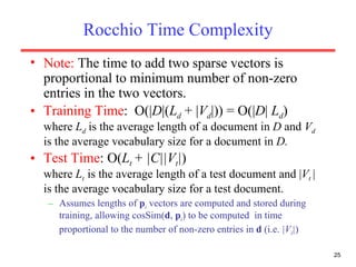
  • 25. Rocchio Time Complexity Note: The time to add two sparse vectors is proportional to minimum number of non-zero entries in the two vectors. Training Time : O(| D |( L d + | V d |)) = O(| D | L d ) where L d is the average length of a document in D and V d is the average vocabulary size for a document in D. Test Time : O( L t + |C||V t | ) where L t is the average length of a test document and | V t | is the average vocabulary size for a test document. Assumes lengths of p i vectors are computed and stored during training, allowing cosSim( d , p i ) to be computed in time proportional to the number of non-zero entries in d (i.e. |V t | )
  • 26. Nearest-Neighbor Learning Algorithm Learning is just storing the representations of the training examples in D . Testing instance x : Compute similarity between x and all examples in D . Assign x the category of the most similar example in D . Does not explicitly compute a generalization or category prototypes. Also called: Case-based Instance-based Memory-based Lazy learning
  • 27. K Nearest-Neighbor Using only the closest example to determine categorization is subject to errors due to: A single atypical example. Noise (i.e. error) in the category label of a single training example. More robust alternative is to find the k most-similar examples and return the majority category of these k examples. Value of k is typically odd to avoid ties, 3 and 5 are most common.
  • 28. Similarity Metrics Nearest neighbor method depends on a similarity (or distance) metric. Simplest for continuous m -dimensional instance space is Euclidian distance . Simplest for m -dimensional binary instance space is Hamming distance (number of feature values that differ). For text, cosine similarity of TF-IDF weighted vectors is typically most effective.
  • 29. 3 Nearest Neighbor Illustration (Euclidian Distance) . . . . . . . . . . .
  • 30. K Nearest Neighbor for Text Training: For each each training example < x , c ( x )>  D Compute the corresponding TF-IDF vector, d x , for document x Test instance y : Compute TF-IDF vector d for document y For each < x , c ( x )>  D Let s x = cosSim( d , d x ) Sort examples, x , in D by decreasing value of s x Let N be the first k examples in D. ( get most similar neighbors ) Return the majority class of examples in N
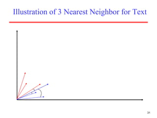
  • 31. Illustration of 3 Nearest Neighbor for Text
  • 32. Rocchio Anomoly Prototype models have problems with polymorphic (disjunctive) categories.
  • 33. 3 Nearest Neighbor Comparison Nearest Neighbor tends to handle polymorphic categories better.
  • 34. Nearest Neighbor Time Complexity Training Time : O(| D | L d ) to compose TF-IDF vectors. Testing Time : O( L t + |D||V t | ) to compare to all training vectors. Assumes lengths of d x vectors are computed and stored during training, allowing cosSim( d , d x ) to be computed in time proportional to the number of non-zero entries in d (i.e. |V t | ) Testing time can be high for large training sets.
  • 35. Nearest Neighbor with Inverted Index Determining k nearest neighbors is the same as determining the k best retrievals using the test document as a query to a database of training documents. Use standard VSR inverted index methods to find the k nearest neighbors. Testing Time : O( B|V t | ) where B is the average number of training documents in which a test-document word appears. Therefore, overall classification is O( L t + B|V t | ) Typically B << | D |
  • 36. Bayesian Methods Learning and classification methods based on probability theory. Bayes theorem plays a critical role in probabilistic learning and classification. Uses prior probability of each category given no information about an item. Categorization produces a posterior probability distribution over the possible categories given a description of an item.
  • 37. Conditional Probability P( A | B ) is the probability of A given B Assumes that B is all and only information known. Defined by: A B
  • 38. Independence A and B are independent iff: Therefore, if A and B are independent: These two constraints are logically equivalent
  • 39. Bayes Theorem Simple proof from definition of conditional probability: QED: (Def. cond. prob.) (Def. cond. prob.)
  • 40. Bayesian Categorization Let set of categories be { c 1 , c 2 ,… c n } Let E be description of an instance. Determine category of E by determining for each c i P( E ) can be determined since categories are complete and disjoint.
  • 41. Bayesian Categorization (cont.) Need to know: Priors: P( c i ) Conditionals: P( E | c i ) P( c i ) are easily estimated from data. If n i of the examples in D are in c i , then P( c i ) = n i / | D| Assume instance is a conjunction of binary features: Too many possible instances (exponential in m ) to estimate all P( E | c i )
  • 42. Naïve Bayesian Categorization If we assume features of an instance are independent given the category ( c i ) ( conditionally independent ). Therefore, we then only need to know P( e j | c i ) for each feature and category.
  • 43. Naïve Bayes Example C = {allergy, cold, well} e 1 = sneeze; e 2 = cough; e 3 = fever E = {sneeze, cough,  fever} 0.4 0.7 0.01 P(fever| c i ) 0.7 0.8 0.1 P(cough| c i ) 0.9 0.9 0.1 P(sneeze| c i ) 0.05 0.05 0.9 P( c i ) Allergy Cold Well Prob
  • 44. Naïve Bayes Example (cont.) P(well | E) = (0.9)(0.1)(0.1)(0.99)/P(E)=0.0089/P(E) P(cold | E) = (0.05)(0.9)(0.8)(0.3)/P(E)=0.01/P(E) P(allergy | E) = (0.05)(0.9)(0.7)(0.6)/P(E)=0.019/P(E) Most probable category: allergy P(E) = 0.0089 + 0.01 + 0.019 = 0.0379 P(well | E) = 0.23 P(cold | E) = 0.26 P(allergy | E) = 0.50 E={sneeze, cough,  fever} 0.4 0.7 0.01 P(fever | c i ) 0.7 0.8 0.1 P(cough | c i ) 0.9 0.9 0.1 P(sneeze | c i ) 0.05 0.05 0.9 P( c i ) Allergy Cold Well Probability
  • 45. Estimating Probabilities Normally, probabilities are estimated based on observed frequencies in the training data. If D contains n i examples in category c i , and n ij of these n i examples contains feature e j , then: However, estimating such probabilities from small training sets is error-prone. If due only to chance, a rare feature, e k , is always false in the training data,  c i :P( e k | c i ) = 0. If e k then occurs in a test example, E , the result is that  c i : P( E | c i ) = 0 and  c i : P( c i | E ) = 0
  • 46. Smoothing To account for estimation from small samples, probability estimates are adjusted or smoothed . Laplace smoothing using an m -estimate assumes that each feature is given a prior probability, p , that is assumed to have been previously observed in a “virtual” sample of size m . For binary features, p is simply assumed to be 0.5.
  • 47. Naïve Bayes for Text Modeled as generating a bag of words for a document in a given category by repeatedly sampling with replacement from a vocabulary V = { w 1 , w 2 ,… w m } based on the probabilities P( w j | c i ). Smooth probability estimates with Laplace m -estimates assuming a uniform distribution over all words ( p = 1/| V |) and m = | V | Equivalent to a virtual sample of seeing each word in each category exactly once.
  • 48. Text Naïve Bayes Algorithm (Train) Let V be the vocabulary of all words in the documents in D For each category c i  C Let D i be the subset of documents in D in category c i P( c i ) = | D i | / | D | Let T i be the concatenation of all the documents in D i Let n i be the total number of word occurrences in T i For each word w j  V Let n ij be the number of occurrences of w j in T i Let P( w i | c i ) = ( n ij + 1) / ( n i + | V |)
  • 49. Text Naïve Bayes Algorithm (Test) Given a test document X Let n be the number of word occurrences in X Return the category: where a j is the word occurring the j th position in X
  • 50. Naïve Bayes Time Complexity Training Time : O(| D | L d + | C || V |)) where L d is the average length of a document in D. Assumes V and all D i , n i , and n ij pre-computed in O(| D | L d ) time during one pass through all of the data. Generally just O(| D | L d ) since usually | C || V | < | D | L d Test Time : O( |C| L t ) where L t is the average length of a test document. Very efficient overall, linearly proportional to the time needed to just read in all the data. Similar to Rocchio time complexity.
  • 51. Underflow Prevention Multiplying lots of probabilities, which are between 0 and 1 by definition, can result in floating-point underflow. Since log( xy ) = log( x ) + log( y ), it is better to perform all computations by summing logs of probabilities rather than multiplying probabilities. Class with highest final un-normalized log probability score is still the most probable.
  • 52. Naïve Bayes Posterior Probabilities Classification results of naïve Bayes (the class with maximum posterior probability) are usually fairly accurate. However, due to the inadequacy of the conditional independence assumption, the actual posterior-probability numerical estimates are not. Output probabilities are generally very close to 0 or 1.
  • 53. Evaluating Categorization Evaluation must be done on test data that are independent of the training data (usually a disjoint set of instances). Classification accuracy : c / n where n is the total number of test instances and c is the number of test instances correctly classified by the system. Results can vary based on sampling error due to different training and test sets. Average results over multiple training and test sets (splits of the overall data) for the best results.
  • 54. N -Fold Cross-Validation Ideally, test and training sets are independent on each trial. But this would require too much labeled data. Partition data into N equal-sized disjoint segments. Run N trials, each time using a different segment of the data for testing, and training on the remaining N  1 segments. This way, at least test-sets are independent. Report average classification accuracy over the N trials. Typically, N = 10.
  • 55. Learning Curves In practice, labeled data is usually rare and expensive. Would like to know how performance varies with the number of training instances. Learning curves plot classification accuracy on independent test data ( Y axis) versus number of training examples ( X axis).
  • 56. N -Fold Learning Curves Want learning curves averaged over multiple trials. Use N -fold cross validation to generate N full training and test sets. For each trial, train on increasing fractions of the training set, measuring accuracy on the test data for each point on the desired learning curve.
  • 57. Sample Document Corpus 600 science pages from the web. 200 random samples each from the Yahoo indices for biology, physics, and chemistry.
  • 58. Sample Learning Curve (Yahoo Science Data)
  • 59. Clustering Partition unlabeled examples into disjoint subsets of clusters , such that: Examples within a cluster are very similar Examples in different clusters are very different Discover new categories in an unsupervised manner (no sample category labels provided).
  • 60. Clustering Example . . . . . . . . . . . . . . . . . . . . . . . . . . . . . . . .
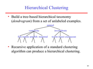
  • 61. Hierarchical Clustering Build a tree-based hierarchical taxonomy ( dendrogram ) from a set of unlabeled examples. Recursive application of a standard clustering algorithm can produce a hierarchical clustering. animal vertebrate fish reptile amphib. mammal worm insect crustacean invertebrate
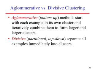
  • 62. Aglommerative vs. Divisive Clustering Aglommerative ( bottom-up ) methods start with each example in its own cluster and iteratively combine them to form larger and larger clusters. Divisive ( partitional, top-down ) separate all examples immediately into clusters.
  • 63. Direct Clustering Method Direct clustering methods require a specification of the number of clusters, k , desired. A clustering evaluation function assigns a real-value quality measure to a clustering. The number of clusters can be determined automatically by explicitly generating clusterings for multiple values of k and choosing the best result according to a clustering evaluation function.
  • 64. Hierarchical Agglomerative Clustering (HAC) Assumes a similarity function for determining the similarity of two instances. Starts with all instances in a separate cluster and then repeatedly joins the two clusters that are most similar until there is only one cluster. The history of merging forms a binary tree or hierarchy.
  • 65. HAC Algorithm Start with all instances in their own cluster. Until there is only one cluster: Among the current clusters, determine the two clusters, c i and c j , that are most similar. Replace c i and c j with a single cluster c i  c j
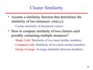
  • 66. Cluster Similarity Assume a similarity function that determines the similarity of two instances: sim ( x , y ). Cosine similarity of document vectors. How to compute similarity of two clusters each possibly containing multiple instances? Single Link : Similarity of two most similar members. Complete Link : Similarity of two least similar members. Group Average : Average similarity between members.
  • 67. Single Link Agglomerative Clustering Use maximum similarity of pairs: Can result in “straggly” (long and thin) clusters due to chaining effect . Appropriate in some domains, such as clustering islands.
  • 69. Complete Link Agglomerative Clustering Use minimum similarity of pairs: Makes more “tight,” spherical clusters that are typically preferable.
  • 71. Computational Complexity In the first iteration, all HAC methods need to compute similarity of all pairs of n individual instances which is O( n 2 ). In each of the subsequent n  2 merging iterations, it must compute the distance between the most recently created cluster and all other existing clusters. In order to maintain an overall O( n 2 ) performance, computing similarity to each other cluster must be done in constant time.
  • 72. Computing Cluster Similarity After merging c i and c j , the similarity of the resulting cluster to any other cluster, c k , can be computed by: Single Link: Complete Link:
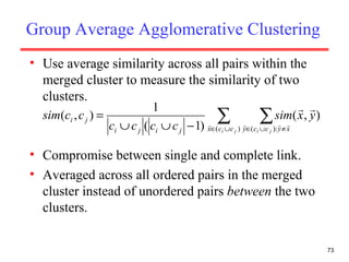
  • 73. Group Average Agglomerative Clustering Use average similarity across all pairs within the merged cluster to measure the similarity of two clusters. Compromise between single and complete link. Averaged across all ordered pairs in the merged cluster instead of unordered pairs between the two clusters.
  • 74. Computing Group Average Similarity Assume cosine similarity and normalized vectors with unit length. Always maintain sum of vectors in each cluster. Compute similarity of clusters in constant time:
  • 75. Non-Hierarchical Clustering Typically must provide the number of desired clusters, k . Randomly choose k instances as seeds , one per cluster. Form initial clusters based on these seeds. Iterate, repeatedly reallocating instances to different clusters to improve the overall clustering. Stop when clustering converges or after a fixed number of iterations.
  • 76. K-Means Assumes instances are real-valued vectors. Clusters based on centroids , center of gravity , or mean of points in a cluster, c : Reassignment of instances to clusters is based on distance to the current cluster centroids.
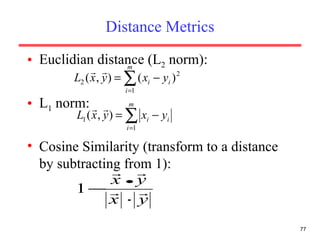
  • 77. Distance Metrics Euclidian distance (L 2 norm): L 1 norm: Cosine Similarity (transform to a distance by subtracting from 1):
  • 78. K-Means Algorithm Let d be the distance measure between instances. Select k random instances { s 1 , s 2 ,… s k } as seeds. Until clustering converges or other stopping criterion: For each instance x i : Assign x i to the cluster c j such that d ( x i , s j ) is minimal. ( Update the seeds to the centroid of each cluster ) For each cluster c j s j =  ( c j )
  • 79. K Means Example (K=2) Reassign clusters Converged! Pick seeds Reassign clusters Compute centroids x x Reasssign clusters x x x x Compute centroids
  • 80. Time Complexity Assume computing distance between two instances is O( m ) where m is the dimensionality of the vectors. Reassigning clusters: O( kn ) distance computations, or O( knm ). Computing centroids: Each instance vector gets added once to some centroid: O( nm ). Assume these two steps are each done once for I iterations: O( Iknm ). Linear in all relevant factors, assuming a fixed number of iterations, more efficient than O(n 2 ) HAC.
  • 81. Seed Choice Results can vary based on random seed selection. Some seeds can result in poor convergence rate, or convergence to sub-optimal clusterings. Select good seeds using a heuristic or the results of another method.
  • 82. Buckshot Algorithm Combines HAC and K-Means clustering. First randomly take a sample of instances of size  n Run group-average HAC on this sample, which takes only O( n ) time. Use the results of HAC as initial seeds for K-means. Overall algorithm is O( n ) and avoids problems of bad seed selection.
  • 83. Text Clustering HAC and K-Means have been applied to text in a straightforward way. Typically use normalized , TF/IDF-weighted vectors and cosine similarity. Optimize computations for sparse vectors. Applications: During retrieval, add other documents in the same cluster as the initial retrieved documents to improve recall. Clustering of results of retrieval to present more organized results to the user ( à la Northernlight folders). Automated production of hierarchical taxonomies of documents for browsing purposes ( à la Yahoo & DMOZ).
  • 84. Soft Clustering Clustering typically assumes that each instance is given a “hard” assignment to exactly one cluster. Does not allow uncertainty in class membership or for an instance to belong to more than one cluster. Soft clustering gives probabilities that an instance belongs to each of a set of clusters. Each instance is assigned a probability distribution across a set of discovered categories (probabilities of all categories must sum to 1).
  • 85. Expectation Maximization (EM) Probabilistic method for soft clustering. Direct method that assumes k clusters: { c 1 , c 2 ,… c k } Soft version of k -means. Assumes a probabilistic model of categories that allows computing P( c i | E ) for each category, c i , for a given example, E . For text, typically assume a naïve-Bayes category model. Parameters  = {P( c i ), P( w j | c i ): i  {1,… k }, j  {1,…,| V |}}
  • 86. EM Algorithm Iterative method for learning probabilistic categorization model from unsupervised data. Initially assume random assignment of examples to categories. Learn an initial probabilistic model by estimating model parameters  from this randomly labeled data. Iterate following two steps until convergence: Expectation (E-step): Compute P( c i | E ) for each example given the current model, and probabilistically re-label the examples based on these posterior probability estimates. Maximization (M-step): Re-estimate the model parameters,  , from the probabilistically re-labeled data.
  • 87. Learning from Probabilistically Labeled Data Instead of training data labeled with “hard” category labels, training data is labeled with “soft” probabilistic category labels. When estimating model parameters  from training data, weight counts by the corresponding probability of the given category label. For example, if P( c 1 | E ) = 0.8 and P( c 2 | E ) = 0.2, each word w j in E contributes only 0.8 towards the counts n 1 and n 1 j , and 0.2 towards the counts n 2 and n 2 j .
  • 88. Naïve Bayes EM Randomly assign examples probabilistic category labels. Use standard naïve-Bayes training to learn a probabilistic model with parameters  from the labeled data. Until convergence or until maximum number of iterations reached: E-Step : Use the naïve Bayes model  to compute P( c i | E ) for each category and example, and re-label each example using these probability values as soft category labels. M-Step : Use standard naïve-Bayes training to re-estimate the parameters  using these new probabilistic category labels.
  • 89. Semi-Supervised Learning For supervised categorization, generating labeled training data is expensive. Idea : Use unlabeled data to aid supervised categorization. Use EM in a semi-supervised mode by training EM on both labeled and unlabeled data. Train initial probabilistic model on user-labeled subset of data instead of randomly labeled unsupervised data. Labels of user-labeled examples are “frozen” and never relabeled during EM iterations. Labels of unsupervised data are constantly probabilistically relabeled by EM.
  • 90. Semi-Supervised Example Assume “quantum” is present in several labeled physics documents, but “Heisenberg” occurs in none of the labeled data. From labeled data, learn that “quantum” is indicative of a physics document. When labeling unsupervised data, label several documents with “quantum” and “Heisenberg” correctly with the “physics” category. When retraining, learn that “Heisenberg” is also indicative of a physics document. Final learned model is able to correctly assign documents containing only “Heisenberg” to physics.
  • 91. Semi-Supervision Results Experiments on assigning messages from 20 Usenet newsgroups their proper newsgroup label. With very few labeled examples (2 examples per class), semi-supervised EM improved accuracy from 27% (supervised data only) to 43% (supervised + unsupervised data). With more labeled examples, semi-supervision can actually decrease accuracy, but refinements to standard EM can prevent this. For semi-supervised EM to work, the “natural clustering of data” must be consistent with the desired categories.
  • 92. Active Learning Select only the most informative examples for labeling. Initial methods: Uncertainty sampling Committee-based sampling Error-reduction sampling
  • 93. Weak Supervision Sometimes uncertain labeling can be inferred. Learning apprentices Inferred feedback Click patterns, reading time, non-verbal cues Delayed feedback Reinforcement learning Programming by Demonstration
  • 94. Prior Knowledge Use of prior declarative knowledge in learning. Initial methods: Explanation-based Learning Theory Refinement Bayesian Priors Reinforcement Learning with Advice
  • 95. Learning to Learn Many applications require learning for multiple, related problems. What can be learned from one problem that can aid the learning for other problems? Initial approaches: Multi-task learning Life-long learning Learning similarity metrics Supra-classifiers