This document presents a nonparametric approach to multiple regression that uses ranks instead of raw values for both the dependent and independent variables. The key points are:
1. It develops a nonparametric multiple regression model using the ranks of observations on the dependent variable and ranks of observations on the independent variables.
2. The method of least squares is applied to the rank-based model to obtain estimates of the regression coefficients.
3. Prediction equations are presented that allow predicting dependent variable ranks based on independent variable ranks.
Bba 3274 qm week 6 part 1 regression modelsStephen Ong
This document provides an overview and outline of regression models and forecasting techniques. It discusses simple and multiple linear regression analysis, how to measure the fit of regression models, assumptions of regression models, and testing models for significance. The goals are to help students understand relationships between variables, predict variable values, develop regression equations from sample data, and properly apply and interpret regression analysis.
Please Subscribe to this Channel for more solutions and lectures
http://www.youtube.com/onlineteaching
Chapter 10: Correlation and Regression
10.2: Regression
This chapter discusses regression models, including simple and multiple linear regression. It covers developing regression equations from sample data, measuring the fit of regression models, and assumptions of regression analysis. Key aspects covered include using scatter plots to examine relationships between variables, calculating the slope, intercept, coefficient of determination, and correlation coefficient, and performing hypothesis tests to determine if regression models are statistically significant. The chapter objectives are to help students understand and appropriately apply simple, multiple, and nonlinear regression techniques.
The document discusses applying machine learning techniques to identify compiler optimizations that impact program performance. It used classification trees to analyze a dataset containing runtime measurements for 19 programs compiled with different combinations of 45 LLVM optimizations. The trees identified optimizations like SROA and inlining that generally improved performance across programs. Analysis of individual programs found some variations, but also common optimizations like SROA and simplifying the control flow graph. Precision, accuracy, and AUC metrics were used to evaluate the trees' ability to classify optimizations for best runtime.
simple linear regression - brief introductionedinyoka
Goal of regression analysis: quantitative description and
prediction of the interdependence between two or more variables.
• Definition of the correlation
• The specification of a simple linear regression model
• Least squares estimators: construction and properties
• Verification of statistical significance of regression model
The document discusses various techniques for fitting curves to data including linear regression, polynomial regression, and linearization of nonlinear relationships.
Linear regression finds the line that best fits a set of data points by minimizing the sum of the squared residuals. The normal equations are derived and solved to determine the slope and intercept. Polynomial regression extends this to find the best-fit polynomial curve through the data. An example shows fitting a second-order polynomial. Nonlinear relationships can sometimes be linearized by a transformation of variables to apply linear regression. Examples demonstrate applying these techniques.
This document discusses various matrix decomposition techniques including least squares, eigendecomposition, and singular value decomposition. It begins with an introduction to the importance of linear algebra and decompositions for applications. Then it provides examples of using least squares to fit curves to data and find regression lines. It defines eigenvalues and eigenvectors and provides examples of eigendecomposition. It also discusses diagonalization of matrices and using the eigendecomposition to raise matrices to powers. Finally, it discusses singular value decomposition and its applications.
The document provides information on correlation and linear regression. It defines correlation as the association between two variables and discusses how the correlation coefficient r measures the strength of this linear association. It then discusses:
- Computing r from sample data
- Testing the hypothesis that r = 0 using a t-test
- Computing the linear regression equation and coefficient of determination
- Using the regression equation to make predictions when there is a significant linear correlation
Two examples are then provided to demonstrate computing r from data, testing for a significant correlation, finding the regression equation, and making a prediction.
Comparing the methods of Estimation of Three-Parameter Weibull distributionIOSRJM
This document compares different methods for estimating the parameters of a three-parameter Weibull distribution from sample data, including graphical methods, trial and error, Jiang/Murthy's approach, and maximum likelihood estimation. It applies these methods to simulated sample data from a Weibull distribution with known parameters to estimate the location, scale, and shape parameters. The trial and error method uses residual sum of squares to select the location parameter that provides the best fit. The maximum likelihood method derives equations that are solved numerically. The results show that all methods can estimate the parameters reasonably well, though accuracy varies depending on the full or censored sample size.
Economics
Curve Fitting
macroeconomics
Curve fitting helps in capturing the trend in the data by assigning a single function
across the entire range.
If the functional relationship between the two quantities being graphed is known to be
within additive or multiplicative constants, it is common practice to transform the data in
such a way that the resulting line is a straight line.(by plotting) A process of quantitatively
estimating the trend of the outcomes, also known as regression or curve fitting, therefore
becomes necessary.
For a series of data, curve fitting is used to find the best fit curve. The produced equation is
used to find points anywhere along the curve. It also uses interpolation (exact fit to the data)
and smoothing.
Some people also refer it as regression analysis instead of curve fitting. The curve fitting
process fits equations of approximating curves to the raw field data. Nevertheless, for a
given set of data, the fitting curves of a given type are generally NOT unique.
Smoothing of the curve eliminates components like seasonal, cyclical and random
variations. Thus, a curve with a minimal deviation from all data points is desired. This
best-fitting curve can be obtained by the method of least squares.
What is curve fitting Curve fitting?
Curve fitting is the process of constructing a curve, or mathematical functions, which possess closest
proximity to the series of data. By the curve fitting we can mathematically construct the functional
relationship between the observed fact and parameter values, etc. It is highly effective in mathematical
modelling some natural processes.
What is a fitting model?
A fit model (sometimes fitting model) is a person who is used by a fashion designer or
clothing manufacturer to check the fit, drape and visual appearance of a design on a
'real' human being, effectively acting as a live mannequin.
What is a model fit statistics?
The goodness of fit of a statistical model describes how well it fits a set of
observations. Measures of goodness of fit typically summarize the discrepancy
between observed values and the values expected under the model in question.
What is a commercial model?
Commercial modeling is a more generalized type of modeling. There are high
fashion models, and then there are commercial models. ... They can model for
television, commercials, websites, magazines, newspapers, billboards and any other
type of advertisement. Most people who tell you they are models are “commercial”
models.
What is the exponential growth curve?
Growth of a system in which the amount being added to the system is proportional to the
amount already present: the bigger the system is, the greater the increase. ( See geometric
progression.) Note : In everyday speech, exponential growth means runaway expansion, such
as in population growth.
Why is population exponential?
Exponential population growth: When resources are unlimited, populations
exhibit exponential growth, resulting in a J-shaped curve.
1) The document discusses simple linear regression using a scatter diagram and data from a study of employees' years of working experience and income.
2) It presents the scatter diagram and shows how to draw a trend line to roughly estimate dependent variable (income) values from the independent variable (years experience).
3) Equations for the least squares linear regression line are provided, including how to calculate the standard error of estimate, which is interpreted as the standard deviation around the regression line.
Simple Regression presentation is a
partial fulfillment to the requirement in PA 297 Research for Public Administrators, presented by Atty. Gayam , Dr. Cabling and Mr. Cagampang
Regression analysis is a mathematical measure of the average relationship between two or more variables in terms of the original units of the data.
In regression analysis there are two types of variables. The variable whose value is influenced or is to be predicted is called dependent variable and the variable which influences the values or is used for prediction, is called independent variable.
In regression analysis independent variable is also known as regressor or predictor or explanatory variable while the dependent variable is also known as regressed or explained variable.
This document discusses principal component analysis (PCA) and its applications in image processing and facial recognition. PCA is a technique used to reduce the dimensionality of data while retaining as much information as possible. It works by transforming a set of correlated variables into a set of linearly uncorrelated variables called principal components. The first principal component accounts for as much of the variability in the data as possible, and each succeeding component accounts for as much of the remaining variability as possible. The document provides an example of applying PCA to a set of facial images to reduce them to their principal components for analysis and recognition.
Lecture Notes in Econometrics Arsen Palestini.pdfMDNomanCh
This document contains lecture notes on introductory econometrics. It introduces the basic regression model and discusses ordinary least squares (OLS) estimation for both the two-variable and multiple variable cases. It also covers assessing goodness of fit, maximum likelihood estimation, approaches to hypothesis testing, and the use of dummy variables. Examples are provided to illustrate key concepts.
Stuck with your Regression Assignment? Get 24/7 help from tutors with Phd in the subject. Email us at [email protected]
Reach us at http://www.HelpWithAssignment.com
- The document discusses principles of least squares adjustment for survey measurements.
- It introduces random error adjustment to account for measurement errors by minimizing the sum of squared residuals.
- The fundamental principle of least squares states that to obtain the most probable values, the sum of squares of the residuals must be minimized.
- It presents examples to demonstrate setting up and solving least squares adjustments through normal equation matrices in both linear and nonlinear systems.
The document describes nonlinear regression models, including exponential, power, and polynomial models. It provides examples of using these models to fit data and find the best-fit parameters. Specifically, it examines using an exponential model to analyze radiation intensity data over time from a medical isotope. It shows setting up the nonlinear equation to solve for the decay rate parameter numerically, calculates the other model constant, and plots the fit. The example also calculates the radiation intensity remaining after 24 hours based on the regression model.
This document provides an overview of regression analysis and compares regression to neural networks. It defines regression as estimating the relationship between variables. The main types covered are linear, nonlinear, simple, multiple and logistic regression. Examples are given to illustrate simple linear regression and least squares methods. The document also discusses best practices like avoiding overfitting and dealing with multicollinearity. Finally, it provides examples comparing regression and deep learning approaches.
Foreign exchange (forex) is a decentralized global market where currencies trade 24/5. It is the largest market by volume at over $5 trillion daily. Forex involves speculating on currency pairs by buying one currency and selling another. For example, buying the EUR/USD pair if expecting the euro to rise against the dollar. Profits are made if the currency is later sold higher than it was bought. Technical analysis tools help traders analyze trends and make trading decisions. Forex leverage allows traders to control large positions with relatively small amounts of capital, but also increases risk.
Investigating the central role that theories of the visual arts and creativity played in the development of fascism in France, Mark Antliff examines the aesthetic dimension of fascist myth-making within the history of the avant-garde. Between 1909 and 1939, a surprising array of modernists were implicated in this project, including such well-known figures as the symbolist painter Maurice Denis, the architects Le Corbusier and Auguste Perret, the sculptors Charles Despiau and Aristide Maillol, the “New Vision” photographer Germaine Krull, and the fauve Maurice Vlaminck.
Infrastructure for Tracking Information Flow from Social Media to U.S. TV New...Himarsha Jayanetti
This study examines the intersection between social media and mainstream television (TV) news with an aim to understand how social media content amplifies its impact through TV broadcasts. While many studies emphasize social media as a primary platform for information dissemination, they often underestimate its total influence by focusing solely on interactions within the platform. This research examines instances where social media posts gain prominence on TV broadcasts, reaching new audiences and prompting public discourse. By using TV news closed captions, on-screen text recognition, and social media logo detection, we analyze how social media is referenced in TV news.
Body temperature_chemical thermogenesis_hypothermia_hypothermiaMetabolic acti...muralinath2
Homeothermic animals, poikilothermic animals, metabolic activities, muscular activities, radiation of heat from environment, shivering, brown fat tissue, temperature, cinduction, convection, radiation, evaporation, panting, chemical thermogenesis, hyper pyrexia, hypothermia, second law of thermodynamics, mild hypothrtmia, moderate hypothermia, severe hypothertmia, low-grade fever, moderate=grade fever, high-grade fever, heat loss center, heat gain center
Vital Vitamins: A Clinical Nutrition Approach to Functions, Deficiency & SourcesSarumathi Murugesan
This presentation, titled "Vital Vitamins: A Clinical Nutrition Approach to Functions, Deficiency & Sources," offers a concise yet comprehensive overview of essential vitamins including A, D, E, K, B-complex, and C, as studied in the fields of clinical nutrition and dietetics.
Designed for students, educators, and healthcare professionals, this resource covers:
Physiological functions of fat- and water-soluble vitamins
Recommended Dietary Allowances (RDA) based on age and life stage
Major dietary sources relevant to practical diet planning
Common deficiency disorders with clinical relevance
Toxicity symptoms and risk of over-supplementation (where applicable)
Ideal for learners preparing for UGC NET, B.Sc. & M.Sc. Nutrition, Nursing, and Allied Health Sciences, this SlideShare simplifies complex content into clear, easy-to-follow slides rooted in evidence-based practice.
They envisioned a brave new world, and what they got was fascism. As vibrant as its counterparts in Paris, Munich, and Milan, the avant-garde of Florence rose on a wave of artistic, political, and social idealism that swept the world with the arrival of the twentieth century. How the movement flourished in its first heady years, only to flounder in the bloody wake of World War I, is a fascinating story, told here for the first time. It is the history of a whole generation's extraordinary promise--and equally extraordinary failure.
The Man Who Dared to Challenge Newton: The True Story of Thane Heins, the Canadian Genius
Who Changed the World
By Johnny Poppi – for international press
In a small town in Ontario, among wheat fields and wind-filled silences, a man has worked for decades in
anonymity, armed only with naive curiosity, motors, copper wires, and questions too big to ignore. His
name is Thane C/ Heins, and according to some scientists who have seen him in action, he may have
made—and indeed has made—the most important scientific discovery in the history of humanity.
A discovery which will eventually eliminate the need for oil, coal, and uranium, and at the very least their
harmful effects while eliminating the need to recharge electric vehicles, and even rewrite—as it has already
begun—the very laws of physics as we’ve known them since Aristotle in 300 BC.
Sound like science fiction? Then listen to this story.
Structure formation with primordial black holes: collisional dynamics, binari...Sérgio Sacani
Primordial black holes (PBHs) could compose the dark matter content of the Universe. We present the first simulations of cosmological structure formation with PBH dark matter that consistently include collisional few-body effects, post-Newtonian orbit corrections, orbital decay due to gravitational wave emission, and black-hole mergers. We carefully construct initial conditions by considering the evolution during radiation domination as well as early-forming binary systems. We identify numerous dynamical effects due to the collisional nature of PBH dark matter, including evolution of the internal structures of PBH halos and the formation of a hot component of PBHs. We also study the properties of the emergent population of PBH binary systems, distinguishing those that form at primordial times from those that form during the nonlinear structure formation process. These results will be crucial to sharpen constraints on the PBH scenario derived from observational constraints on the gravitational wave background. Even under conservative assumptions, the gravitational radiation emitted over the course of the simulation appears to exceed current limits from ground-based experiments, but this depends on the evolution of the gravitational wave spectrum and PBH merger rate toward lower redshifts.
2025 Insilicogen Company Korean BrochureInsilico Gen
Insilicogen is a company, specializes in Bioinformatics. Our company provides a platform to share and communicate various biological data analysis effectively.
A tale of two Lucies: talk at the maths dept, Free University of AmsterdamRichard Gill
Despite the title, this talk will focus on the case of Lucy Letby. It focusses on the way the police investigation determined "suspicious incidents" and enters into the actual medical condition of those babies. I hope to also discuss the mathematics of sandwich ELISA immunoassay and of neonatal insulin metabolism.
Direct Evidence for r-process Nucleosynthesis in Delayed MeV Emission from th...Sérgio Sacani
The origin of heavy elements synthesized through the rapid neutron capture process (r-process) has been an enduring mystery for over half a century. J. Cehula et al. recently showed that magnetar giant flares, among the brightest transients ever observed, can shock heat and eject neutron star crustal material at high velocity, achieving the requisite conditions for an r-process.A. Patel et al. confirmed an r-process in these ejecta using detailed nucleosynthesis calculations. Radioactive decay of the freshly synthesized nuclei releases a forest of gamma-ray lines, Doppler broadened by the high ejecta velocities v 0.1c into a quasi-continuous spectrum peaking around 1 MeV. Here, we show that the predicted emission properties (light curve, fluence, and spectrum) match a previously unexplained hard gamma-ray signal seen in the aftermath of the famous 2004 December giant flare from the magnetar SGR 1806–20. This MeV emission component, rising to peak around 10 minutes after the initial spike before decaying away over the next few hours, is direct observational evidence for the synthesis of ∼10−6 Me of r-process elements. The discovery of magnetar giant flares as confirmed r-process sites, contributing at least ∼1%–10% of the total Galactic abundances, has implications for the Galactic chemical evolution, especially at the earliest epochs probed by low-metallicity stars. It also implicates magnetars as potentially dominant sources of heavy cosmic rays. Characterization of the r-process emission from giant flares by resolving decay line features offers a compelling science case for NASA’s forthcomingCOSI nuclear spectrometer, as well as next-generation MeV telescope missions.
Examining Visual Attention in Gaze-Driven VR Learning: An Eye-Tracking Study ...Yasasi Abeysinghe
This study presents an eye-tracking user study for analyzing visual attention in a gaze-driven VR learning environment using a consumer-grade Meta Quest Pro VR headset. Eye tracking data were captured through the headset's built-in eye tracker. We then generated basic and advanced eye-tracking measures—such as fixation duration, saccade amplitude, and the ambient/focal attention coefficient K—as indicators of visual attention within the VR setting. The generated gaze data are visualized in an advanced gaze analytics dashboard, enabling us to assess users' gaze behaviors and attention during interactive VR learning tasks. This study contributes by proposing a novel approach for integrating advanced eye-tracking technology into VR learning environments, specifically utilizing consumer-grade head-mounted displays.
3. http://numericalmethods.eng.usf.edu 3
What is Regression?
What is regression? Given n data points
best fit )
(x
f
y = to the data.
Residual at each point is
)
(x
f
y =
Figure. Basic model for regression
)
,
(
),......,
,
(
),
,
( 2
2
1
1 n
n y
x
y
x
y
x
)
( i
i
i x
f
y
E −
=
y
x
)
,
( 1
1 y
x
)
,
( n
n y
x
)
,
( i
i y
x
)
( i
i
i x
f
y
E −
=
4. http://numericalmethods.eng.usf.edu 4
Linear Regression-Criterion#1
Given n data points best fit x
a
a
y 1
0 +
= to the data.
Does minimizing∑
=
n
i
i
E
1
work as a criterion?
x
x
a
a
y 1
0 +
=
)
,
( 1
1 y
x
)
,
( 2
2 y
x
)
,
( 3
3 y
x
)
,
( n
n y
x
)
,
( i
i y
x
i
i
i x
a
a
y
E 1
0 −
−
=
y
Figure. Linear regression of y vs x data showing residuals at a typical point, xi .
)
,
(
),......,
,
(
),
,
( 2
2
1
1 n
n y
x
y
x
y
x
5. http://numericalmethods.eng.usf.edu 5
Example for Criterion#1
x y
2.0 4.0
3.0 6.0
2.0 6.0
3.0 8.0
Example: Given the data points (2,4), (3,6), (2,6) and (3,8), best fit
the data to a straight line using Criterion#1
Figure. Data points for y vs x data.
Table. Data Points
0
2
4
6
8
10
0 1 2 3 4
y
x
Minimize∑
=
n
i
i
E
1
8. http://numericalmethods.eng.usf.edu 8
Linear Regression – Criterion #1
0
4
1
=
∑
=
i
i
E for both regression models of y=4x-4 and y=6
The sum of the residuals is minimized, in this case it is zero,
but the regression model is not unique.
Hence the criterion of minimizing the sum of the residuals is a
bad criterion.
0
2
4
6
8
10
0 1 2 3 4
y
x
11. http://numericalmethods.eng.usf.edu 11
Example for Criterion#2
x y
2.0 4.0
3.0 6.0
2.0 6.0
3.0 8.0
Example: Given the data points (2,4), (3,6), (2,6) and (3,8), best fit
the data to a straight line using Criterion#2
Figure. Data points for y vs. x data.
Table. Data Points
0
2
4
6
8
10
0 1 2 3 4
y
x
Minimize ∑
=
n
i
i
E
1
|
|
15. http://numericalmethods.eng.usf.edu 15
Least Squares Criterion
The least squares criterion minimizes the sum of the square of the
residuals in the model, and also produces a unique line.
( )
2
1
1
0
1
2
∑ −
−
=
∑
=
=
=
n
i
i
i
n
i
i
r x
a
a
y
E
S
x
1
1
, y
x
2
2
, y
x
3
3
, y
x
n
n
y
x ,
i
i
y
x ,
y
Figure. Linear regression of y vs x data showing residuals at a typical point, xi .
x
a
a
y 1
0 +
=
i
i
i x
a
a
y
E 1
0 −
−
=
1
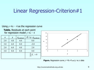
6. http://numericalmethods.eng.usf.edu
16
Finding Constants of Linear Model
( )
2
1
1
0
1
2
∑ −
−
=
∑
=
=
=
n
i
i
i
n
i
i
r x
a
a
y
E
S
Minimize the sum of the square of the residuals:
To find
( )( ) 0
1
2
1
1
0
0
=
−
−
−
−
=
∂
∂
∑
=
n
i
i
i
r
x
a
a
y
a
S
( )( ) 0
2
1
1
0
1
=
−
−
−
−
=
∂
∂
∑
=
n
i
i
i
i
r
x
x
a
a
y
a
S
giving
i
n
i
i
i
n
i
i
n
i
x
y
x
a
x
a ∑
∑
∑ =
=
=
=
+
1
2
1
1
1
0
0
a and 1
a we minimize with respect to 1
a 0
a
and
r
S .
∑
∑
∑ =
=
=
=
+
n
i
i
i
n
i
n
i
y
x
a
a
1
1
1
1
0
17. http://numericalmethods.eng.usf.edu
17
Finding Constants of Linear Model
0
a
Solving for
2
1
1
2
1
1
1
1
−
−
=
∑
∑
∑
∑
∑
=
=
=
=
=
n
i
i
n
i
i
n
i
i
n
i
i
n
i
i
i
x
x
n
y
x
y
x
n
a
and
2
1
1
2
1
1
1
1
2
0
−
−
=
∑
∑
∑
∑
∑
∑
=
=
=
=
=
=
n
i
i
n
i
i
n
i
i
i
n
i
i
n
i
i
n
i
i
x
x
n
y
x
x
y
x
a
1
a
and directly yields,
x
a
y
a 1
0 −
=
18. http://numericalmethods.eng.usf.edu
18
Example 1
The torque, T needed to turn the torsion spring of a mousetrap through
an angle, is given below.
Angle, θ Torque, T
Radians N-m
0.698132 0.188224
0.959931 0.209138
1.134464 0.230052
1.570796 0.250965
1.919862 0.313707
Table: Torque vs Angle for a
torsional spring
Find the constants for the model given by
θ
2
1 k
k
T +
=
Figure. Data points for Torque vs Angle data
0.1
0.2
0.3
0.4
0.5 1 1.5 2
θ (radians)
Torque
(N-m)
19. http://numericalmethods.eng.usf.edu
19
Example 1 cont.
1
a
The following table shows the summations needed for the calculations of
the constants in the regression model.
θ 2
θ θ
T
Radians N-m Radians2 N-m-Radians
0.698132 0.188224 0.487388 0.131405
0.959931 0.209138 0.921468 0.200758
1.134464 0.230052 1.2870 0.260986
1.570796 0.250965 2.4674 0.394215
1.919862 0.313707 3.6859 0.602274
6.2831 1.1921 8.8491 1.5896
Table. Tabulation of data for calculation of important
∑
=
=
5
1
i
5
=
n
Using equations described for
2
5
1
5
1
2
5
1
5
1
5
1
2
−
−
=
∑
∑
∑
∑
∑
=
=
=
=
=
i
i
i
i
i
i
i
i
i
i
i
n
T
T
n
k
θ
θ
θ
θ
( ) ( )( )
( ) ( )2
2831
6
8491
8
5
1921
1
2831
6
5896
1
5
.
.
.
.
.
−
−
=
2
10
6091
9 −
×
= . N-m/rad
summations
0
a
T
and with
27. http://numericalmethods.eng.usf.edu
27
Linear Regression (special case cont.)
∑
∑
=
=
= n
i
i
n
i
i
i
x
y
x
a
1
2
1
1
( )
∑
=
+
−
=
n
i
i
i
i
r
x
a
x
y
da
dS
1
2
1
1
2
2
0
2
1
2
2
1
2
>
= ∑
=
n
i
i
r
x
da
S
d
∑
∑
=
=
= n
i
i
n
i
i
i
x
y
x
a
1
2
1
1
Does this value of a1 correspond to a local minima or local
maxima?
Yes, it corresponds to a local minima.
29. http://numericalmethods.eng.usf.edu
29
Example 2
Strain Stress
(%) (MPa)
0 0
0.183 306
0.36 612
0.5324 917
0.702 1223
0.867 1529
1.0244 1835
1.1774 2140
1.329 2446
1.479 2752
1.5 2767
1.56 2896
To find the longitudinal modulus of composite, the following data is
collected. Find the longitudinal modulus,
Table. Stress vs. Strain data
E using the regression model
ε
σ E
= and the sum of the square of the
0.0E+00
1.0E+09
2.0E+09
3.0E+09
0 0.005 0.01 0.015 0.02
Strain, ε (m/m)
Stress,
σ
(Pa)
residuals.
Figure. Data points for Stress vs. Strain data
30. http://numericalmethods.eng.usf.edu
30
Example 2 cont.
i ε σ ε 2 εσ
1 0.0000 0.0000 0.0000 0.0000
2 1.8300×10⁻³ 3.0600×10⁸ 3.3489×10⁻⁶ 5.5998×10⁵
3 3.6000×10⁻³ 6.1200×10⁸ 1.2960×10⁻⁵ 2.2032×10⁶
4 5.3240×10⁻³ 9.1700×10⁸ 2.8345×10⁻⁵ 4.8821×10⁶
5 7.0200×10⁻³ 1.2230×10⁹ 4.9280×10⁻⁵ 8.5855×10⁶
6 8.6700×10⁻³ 1.5290×10⁹ 7.5169×10⁻⁵ 1.3256×10⁷
7 1.0244×10⁻² 1.8350×10⁹ 1.0494×10⁻⁴ 1.8798×10⁷
8 1.1774×10⁻² 2.1400×10⁹ 1.3863×10⁻⁴ 2.5196×10⁷
9 1.3290×10⁻² 2.4460×10⁹ 1.7662×10⁻⁴ 3.2507×10⁷
10 1.4790×10⁻² 2.7520×10⁹ 2.1874×10⁻⁴ 4.0702×10⁷
11 1.5000×10⁻² 2.7670×10⁹ 2.2500×10⁻⁴ 4.1505×10⁷
12 1.5600×10⁻² 2.8960×10⁹ 2.4336×10⁻⁴ 4.5178×10⁷
1.2764×10⁻³ 2.3337×10⁸
Table. Summation data for regression model
∑
=
12
1
i
∑
=
−
×
=
12
1
3
2
10
2764
.
1
i
i
ε
∑
=
×
=
12
1
8
10
3337
.
2
i
i
iε
σ
∑
∑
=
=
= 12
1
2
12
1
i
i
i
i
i
E
ε
ε
σ
3
8
10
2764
.
1
10
3337
.
2
−
×
×
=
GPa
84
.
182
=
∑
∑
=
=
= n
i
i
n
i
i
i
E
1
2
1
ε
ε
σ
32. Additional Resources
For all resources on this topic such as digital audiovisual
lectures, primers, textbook chapters, multiple-choice
tests, worksheets in MATLAB, MATHEMATICA, MathCad
and MAPLE, blogs, related physical problems, please
visit
http://numericalmethods.eng.usf.edu/topics/linear_regr
ession.html