SlideShare a Scribd company logo
By
(Prof)Dr. Maya Nayak
 Introduction
The explosive growth in data and databases has generated
an urgent need for new techniques and tools that can
intelligently and automatically transform the processed
data into useful information and knowledge.
Consequently, data mining has become a research area
with increasing importance.
What is Data Mining ?
Data mining is nothing but the knowledge discovery in
databases, that means a process of nontrivial extraction of
implicit, previously unknown and potentially useful
information (such as knowledge rules, constraints,
regularities) from data in databases.
A data-mining algorithm constitutes a model, a
preference criterion, and a search algorithm. The
more common model functions in data mining
include classification, clustering, rule generation
and knowledge discovery
 What is Knowledge Discovery in Databases (KDD)?
Extraction of meaningful information from a large
database.
Data
Selection
Data
Compression
Data
formatting
Data Mining
KDD
Raw voltage
Data samples
Overall KDD block diagram
 What is time series data mining ?
A time series data is nothing but the data varies with time.
 Two types of time series data:
1. Periodic data
2. Non-stationary data
Examples of Non-stationary data:
 Seismic signal
 Power signal
 Speech signal
 Radar signal
 Biomedical signal and fluctuating data occurring in
business, financial markets including stocks, etc
 Existing Research work ?
 Objective of the thesis :
In this thesis is focused on the application of data
mining concepts to power network signal
disturbance time series, the approach is a general
one and can be applied to any time varying and non-
stationary data that arises in different fields of
science and engineering.
Data Mining Block diagram
Figure to be inserted from
published paper
Thus the main objective of the thesis is summarized as
1. Feature vector selection in data mining using
advanced signal processing techniques using Wavelet
transform and S-transform.
2. Developing a S-Transform based new hybrid K-
means and Particle Swarm Optimizer for data
clustering and classification in time series data mining.
Developing new Neural and Neuro-Fuzzy classifiers for
classification in data mining.
* Wavelet transform
* S-Transform
Fourier Transform
The Fourier Transform is one of the oldest and most
powerful tools in signal processing. This transform
maps the signal in time domain to a frequency domain.
The Fourier Transform of a signal is given as:
2
( ) ( ) i ft
Y f y t e dt



 
2
( ) ( ) i ft
y t Y f e df


 
Discrete version of FT is DFT of a time series of
length N is
21
0
1
[ ]
i nkTN
NT
k
n
Y y kT e
NT N
 

 
  

where T is the sampling interval.
Short Time Fourier Transform (STFT)
  2
, ( ) ( ) i ft
STFT f y t w t e dt
 



 
 Wavelet Transform and Multi-resolution
analysis
*
,( , ) ( ) ( )a bW a b y t t dt


 
where is any square integrable function, a is the scaling
parameter, b is the translation parameter and is the
dilation and translation of the mother wavelet.
, ( )a b t
( )y t
,
1
( )a b
t b
t
aa
 
 
  
 
Phase Corrected Wavelet: S-Transform
  2
( , ) ( ) , i ft
S f y t g t f e 
 



 
where the Gaussian modulation function g( , f) is given by
2
2
2
( , )
2
t
f
g f e 




with the spread parameter inversely proportional to the
frequency
1
f
 
The final expression becomes
2 2
( )
22
( , ) ( )
2
t f
i ftf
S f y t e e dt




 



 
To increase the frequency resolution, the spread of the Gaussian
window  is written as
f

 
and the generalized S-Transform is obtained as
2 2
2
( )
22
( , ) ( )
2
t f
i ftf
S f y t e e dt



 




 
Implementation of S-Transform (ST)
The computation of the S-Transform is efficiently implemented
using the convolution theorem and FFT. The following steps are
used for the computation of S-Transform:
1. Compute the DFT of the signal y(k) using FFT software
routine and shift spectrum Y[m] to Y[m+n].
2. Compute the Gaussian window function for
the required frequency n.
3. Compute the inverse Fourier Transform of the product of DFT
and Gaussian window function to give the ST matrix.
2 2 2 2
exp(-2π β m /n )
Comparison between DWT and S-Transform for
Analysis of Time Series Events
(a)Oscillatory transient (b) S-Transform output of oscillatory
transient
(a)
(b)
(a) Oscillatory transient (b) Level 4 detail coefficients (c) Level 3
detail coefficients (d) Level 2 detail coefficients (e) Level 1 detail
coefficients
(a) Swell (b) S-Transform output of voltage swell
(a) Swell (b) Level 4 detail coefficients (c) Level 3 detail coefficients
(d) Level 2 detail coefficients (e) Level 1 detail coefficients
Feature Extraction
Disturbances F1 F2 F3 F4 F5
Normal 1.002
Sag (60%) 0.593 0.053 .031 .0312 50.0
Swell (50%) 1.50 0.012
9
.076 .015 50
Momentary
Interruption (MI)
(5%)
0.0724 0.035 .019 .0350 50
Harmonics
(0% 3rd + 10% 5th)
1.0 0.033
9
.0556 .141 50
Sag with Harmonic
(60%)
0.601 .0228 .0408 .1139 50
Swell with Harmonic
(50%)
1.5 .0219 .079 .1155 50
Flicker (5 Hz, 4%) 0.987 .0168 .026 0.0186 55
Sag (60%) .591 .022 .039 .027 50
Swell (50%) 1.503 .012 .076 .029 50
Momentary
Interruption (MI)
.070 .0387 .0323 .044 50
Harmonics 1.032 .050 .064 0.25 50
Sag with Harmonic
(60%)
0.601 .0228 .0408 0.1139 50
Swell with Harmonic
(50%)
1.50 .0219 .079 .1155 50
Flicker (4%, 5 Hz) .998 .0209 .027 0.1159 55
Notch + harmonics .940 .1275 .0531 0.198 50
Spike + harmonics 1.072 .141 .066 .204 50
Transient
(low frequency)
1.021 0.1473 .0148 .0566 440
Table- 3: Effects of Window parameter α
Steady state variations Transient variations
Factor  F1 F2 F1 F2
0.4 0.602 0.0427 0.9877 0.1654
0.6 0.610 0.0236 0.9898 0.1650
0.8 0.621 0.01735 0.9911 0.1647
1 0.633 0.0145 0.9923 0.1623
1.2 0.645 0.0126 0.9927 0.1600
 Conclusion
 Introduction
The goal of clustering is to identify the structure of an
unlabeled data set by objectively organizing data into
homogenous groups where the within-group-object
similarity is minimized and between the groups object-
dissimilarity is maximized. The clustering aims at
identifying and extracting significant groups in
underlying data.
Time series clustering using feature based approach.
Feature
Extraction (ST
or WT)
Clustering
algorithm
Time series ClustersFeatures
Model based Clustering
Discretization Modeling
Modeling Clustering
Model
parameters
Cluster
Centres
Coefficients of Residualsraw materials
K-Means Clustering
},...,2,1(},,...,2,1{, KjNizxd ji 


ji Cx
i
j
j Kjx
N
z ,...,2,1,
1
where zj is the jth cluster center. The necessary
condition of the minimum J is
where Nj is the number of points belonging to cluster
Cj.
PSO (Particle Swarm Optimization)
The aim of the PSO is to find the particle position that
results in the best evaluation of a given fitness (objective)
function. Each particle represents a position in Nd
dimensional space, and is “flown” through this multi-
dimensional search space, adjusting its position towards
both.
 the particle’s best position found thus far, and
 the best position in the neighborhood of that particle.
Each particle i maintains the following information:
 xi : The current position of the particle;
 vi : The current velocity of the particle ;
yi : The personal best position of the particle.
, , 1 1, , 2 2, ,
ˆ( 1) ( ) ( ) ( ( )) ( )( ( ) ( ))i k i k k i k k k i kv t wv t c r t y x t c r t y t x t      
( 1) ( ) ( 1)i i ix t x t v t   
where w is the inertia weight c1 and c2 are the acceleration
constants, , and k=1,…,Nd.1, ( )kr t 2, ( ) ~ (0,1),jr t U
PSO Clustering
In the context of clustering, a single particle represents the Nc cluster
centroid vectors. That is, each particle xi is constructed as follows:
1 1( ,..., ,..., )ci i j iNx m m m
where mi1 refers to the j-th cluster centroid vector of the i-th particle in cluster
Cij. The fitness of particles is easily measured as the quantization error,
1 ( , ) /p ij
Nc
j Z C p j ij
e
c
d z m C
J
N
  
  
 
where is the number of data vectors belonging to cluster Cij.ijC
gbest PSO Cluster Algorithm
1. Initialize each particle to contain Nc randomly selected cluster
centroids.
Calculate the Euclidean distance d(zp , mij) to all cluster
centroids Cij.
Using the above notation, the standard K-means algorithm is
summarized as
1. Randomly initialize the Nc cluster centroid vectors.
2. Repeat
(a) For each data vector, assign the vector to the class with
the closest centroid vector, where the distance to the centroid is
determined using
(b) Recalculate the cluster centroid vectors, using
1
p j
j p
Z Cj
m z
n  
 
until a stopping criterion is satisfied.
(ii) Assign zp to cluster Cij such that
(i)
 1,...,( , ) min ( , )cp ij c N p icd z m d z m 
(1)
(2)
(iii) Calculate the global best and local best positions
c) Update the global best and local best positions
d) Update the cluster centroids using equations (1) and (2).
where tmax is the maximum number of iterations.
Hybrid PSO Algorithm
It is based on the passive congregation and a kind of coordinated
aggregation observed in the swarms known as GPAC-PSO and
modifying it further to yield GPAC-Adaptive PSO or simply to be
known as GPAC-APSO.
The swarms of the enhanced GPAC is manipulated by the velocity
update
 1 1 2 2 3 3( 1) . ( ). ( ) . .( ( ) . .( ( )) . .( ( ))i i i i k i r iv t k w t v t c rand P S t c rand P S t c rand P S t       
where i = 1, 2,…, N; c1, c2, and c3 are the cognitive, social, and
passive congregation parameters, respectively; rand1, rand2, and
rand3 are random numbers uniformly distributed within [0,1]; Pi is
the best previous position of the ith particle; Pk is either the global
best position ever attained among all particles in the case of
enhanced GPAC and Pr is the position of passive congregator
(position of a randomly chosen particle-r).
 the quantization error
 the intra-cluster distances, i.e. the distance between
data vectors within a cluster, where the objective is to
minimize the intra-cluster distances;
 the inter-cluster distances, i.e. the distance between the
centroids of the clusters, where the objective is to
maximize the distance between clusters.
w=0.72 and c1=c2=1.49 to ensure good convergence.
(a) F1- F2 K-Means PSO
Cluster-4
Cluster-3
Cluster-1
Cluster-2
HYBRID PSO OUTPUT :
Cluster 1 Sag
Cluster 2: Swell
Cluster 3: Normal + harmonic
Cluster 4: Transient + Notch
GBEST PSO OUTPUT
(b) F1 - F2 GBEST PSO
Cluster-1
Cluster-4
Cluster-3Cluster-2
GBEST PSO OUTPUT
Cluster 1 Sag
Cluster 2: Swell
Cluster 3: Normal + harmonic
Cluster 4: Transient + Notch
(c) F1- F2 GPAC APSO
GPAC APSO OUTPUT
Cluster-4
Cluster-1
Cluster-3
Cluster-2
Cluster 1 Sag
Cluster 2: Swell
Cluster 3: Normal + harmonic
Cluster 4: Transient + Notch
F1 - F2 Fitness Plots
GPAC APSO
PSO
K-Means
GBEST PSOGPAC APSO
K-Means
PSO
GPAC-APSO
GBEST PSO
The proposed method is very efficient and simple to
implement for clustering analysis when the number of
clusters is known a priori. The modified GPAC-PSO
known as GPAC-APSO is found to be more efficient and
has a quick convergence property in comparison to other
PSO variants.
The next step in this research is to transform the
visually distinguishable patterns to feature vectors
that can be used by classifiers such as neural
networks to automatically classify the
disturbances.
*
In order to improve the classification accuracy a novel neural
architecture comprising hybrid combinations of the radial basis
function neural network and a functional link network that provides
a more robust pattern recognizer for non-stationary time series data
is undertaken for detailed study.
Signal
S-transform
Feature
extraction
Neural
Network
Display recognized
patterns
PO
ST
PR
OC
ESS
I
NG
A Neural network architecture is used to test the efficacy
of the proposed method.
 
2
1


Q
j
ij xdE
)()1( kEk w  
where Q is the number of training samples and the
weights are updated as
where wE is the gradient with respect to weight, and  is
the momentum constant, and  is the learning rate.
It consists of a radial basis layer and a competitive layer.
FIGURE 4.3
TO INSERT
where
i number of input layers;
h number of hidden layers
j number of output layers;
k number of training examples;
Nk number of classification (clusters);
σ smoothing parameters (standard deviation), 0.1< σ <1
X input vector;
The algorithm of the inference output vector Y in the PNN is as
follows:
1
. and ,hy hy
j hj h j hj
h hj
net W H N W
N
  
max( ) then 1, else 0j k j j
k
net net Y Y  If
Euclidean distance between the vectors X and Xkj,
 
2
kj i kji
X X X X  
connection weight between the input layer X and the hidden layer
H;
is the connection weight between the hidden layer H and the output
layer Y.
xh
ihW
hy
hjW
We use RBFs with the random vector functional link nets
(RVFLNs) to obtain the powerful radial basis functional
link nets (RBFLNs).
As RBFNN represents a nonlinear model while the RBFLN
includes that nonlinear model as well as a linear model
(the direct lines from the input to output nodes) so that the
linear parts of a mapping do not need to be approximated
by the nonlinear model.
Radial Basis Functional Link Net (RBFLN)
For an input vector , the output of th output node produced by
an RBF is given by
  

 

11
11
)(
1 1
)(
2
)()()(
m
n
noj
m
i i
ctx
ij
m
i
m
n
nojiijj txwewtxwtwto
i


where is the center of the ‘i’ th hidden node, is the width
of the ‘i’th center, and is the total number of hidden
nodes.
If output of the hidden neurons, by vector notation
))t(....,),........t(),t(( tot 21
and weight vector for the hidden RBF units
)w,......,w,w(w mjj2j1j  and the weight vector for the linear units
)w,.......,w,w(w mjj2j1j

RBFLN output can be written as
j
T
jj wwo 
The sets of centers are trained with K-means clustering
approach, where the centers are initially defined as the first
training inputs that correspond to a specific class . The
Centroid vector is given by
 )c(x.,),........c(x),c(x)i(C mcc 210 
c
At each iteration , following a new input is presented,
the distance for each of the centers is denoted by
i )(ix
)i(jj c)i(x)i( 1 cm...,,.........2,1j where
The kth center is updated by the following equation:
)i()i(C)i(C kkk  1
k is chosen in such a way that it minimizes )(ij
)i(arg(min(k jThus
and is the learning rate.
The width associated with the k th center is adjusted as
2
1
1


aN
j
jkk )i(C)i(C
N
)i(
Where N is the number of hidden neurons.
Wavelet based Neural Classification Schemes
Method-1 (WT-1) was implemented using the thirteen level coiflet
5-wavelet decomposition. The de-noising step in Method-2(WT-2)
was omitted to test its effectiveness in noise. A hybrid DFT-DWT
fuzzy expert system approach known as Method-3 (WT-3) is also
considered in this paper for feature extraction and disturbance
pattern classification.
Distortionclassificationinwaveletdomain
Block diagram of classification algorithm
The important features obtained from the Fourier (DFT) and wavelet analysis
(DWT) for the non-stationary disturbance time series data are listed as follows:
1 Fundamental and harmonic components obtained from the Discrete
Fourier Transform of the time series signal data samples.
2. The phase angle shift of the disturbance time series with respect to
normal waveform Ln.
3. Number of peaks of the wavelet coefficients (Nn).
4. Energy of the wavelet coefficients (Ewn).
5. Oscillation number of missing voltage time series data.
The extracted features are then used with different types of
neural classifiers such as multilayered perceptron network,
probabilistic neural network, and proposed radial basis
functional link network for pattern classification, data
mining and subsequent knowledge discovery.
MLP Pure 30dB
Method WT-1 WT-2 ST WT-1 WT-2 ST
Oscillatory transient 95% 95% 90% 30% 90% 95%
Impulsive transient 100% 70% 95% 100% 65% 85%
Multiple notch 100% 85% 100% 90% 85% 100%
Voltage swell 100% 100% 100% 55% 95% 100%
Voltage sag 90% 80% 80% 60% 85% 96%
Interruption 100% 90% 100% 100% 95% 100%
Harmonics 100% 85% 90% 15% 80% 85%
Swell +
harmonics 100% 95% 100% 60% 95% 100%
Sag +harmonics 100% 80% 100% 25% 80% 100%
Average 98.33% 86.67% 95% 59.44% 85.56% %
RBFLN Pure 30dB
Method WT-1 WT-2 ST WT-1 WT-2 ST
Oscillatory
transient 95% 95% 80% 45% 30% 90%
Impulsive
transient 100% 75% 100% 95% 65% 70%
Multiple notch 85% 85% 90% 85% 85% 95%
Voltage swell 100% 95% 90% 75% 95% 90%
Voltage sag 85% 85% 80% 80% 85% 70%
Interruption 100% 100% 100% 25% 100% 100%
Harmonics 100% 95% 90% 5% 80% 90%
Swell
+harmonics 100% 100% 100% 50% 100% 100%
Sag+harmonics 80% 85% 100% 55% 85% 100%
Method WT-1 WT-2 ST WT-1 WT-2 ST
Oscillatory
transient 95% 95% 95% 35% 15% 80%
Impulsive
transient 100% 65% 95% 100% 70% 60%
Multiple notch 100% 85% 90% 90% 90% 95%
Voltage swell 100% 100% 90% 50% 100% 85%
Voltage sag 75% 85% 80% 35% 85% 75%
Interruption 100% 100% 100% 100% 100% 100%
Harmonics 95% 90% 90% 25% 85% 90%
Swell+
harmonics 85% 100% 100% 45% 100% 100%
Sag+harmonics 60% 80% 75% 45% 75% 70%
Average 90% 88.89% 90.56% 58.33% 80% 83.89%
Type of time
series data
Number of
disturbances
Number of class
correctly identified
WT-3 ST
Sag 100 99 92
Swell 100 100 96
Interruption 100 100 97
Harmonics 100 98 95
Switching
transients
100 95 90
Impulse 100 92 97
Flicker 100 99 96
Notch 100 100 94
Average 100% 97.87% 94.62%
Mining of time series data base using fuzzy neural information systems
Ad

Recommended

PDF
Automatic digital modulation recognition using articial
Hemant Ingale
 
PDF
Adaptive dynamic programming algorithm for uncertain nonlinear switched systems
International Journal of Power Electronics and Drive Systems
 
PDF
A Simple Design to Mitigate Problems of Conventional Digital Phase Locked Loop
CSCJournals
 
PPTX
Radix-2 DIT FFT
Sarang Joshi
 
PDF
DIGITAL IMAGE PROCESSING - Day 4 Image Transform
vijayanand Kandaswamy
 
PDF
Decimation in Time
SURAJ KUMAR SAINI
 
PPTX
Unit ii
Chetan Selukar
 
PDF
Ml srhwt-machine-learning-based-superlative-rapid-haar-wavelet-transformation...
Jumlesha Shaik
 
PPTX
Radio Signal Classification with Deep Neural Networks
Kachi Odoemene
 
PDF
第13回 配信講義 計算科学技術特論A(2021)
RCCSRENKEI
 
PDF
Stochastic Alternating Direction Method of Multipliers
Taiji Suzuki
 
PDF
Improving initial generations in pso algorithm for transportation network des...
ijcsit
 
PPTX
Image transforms
11mr11mahesh
 
PDF
ISCAS2013_v5
Chih-Tsung Shen
 
PDF
Minimax optimal alternating minimization \\ for kernel nonparametric tensor l...
Taiji Suzuki
 
PDF
Report01_rev1
Shashidhar Sanda
 
PDF
jammer_placement
M. Reza Gholami
 
PDF
Digital Signal Processing Tutorial:Chapt 3 frequency analysis
Chandrashekhar Padole
 
PDF
Slide tesi
Nicolò Savioli
 
PDF
Neural Networks: Least Mean Square (LSM) Algorithm
Mostafa G. M. Mostafa
 
PDF
El text.tokuron a(2019).jung190711
RCCSRENKEI
 
PPTX
Group01_Project3
Shashidhar Sanda
 
PDF
EE443 - Communications 1 - Lab 1 - Loren Schwappach.pdf
Loren Schwappach
 
PDF
CUDA and Caffe for deep learning
Amgad Muhammad
 
PDF
Real Time Results of a Fuzzy Neural Network Active Noise Controller
IRJET Journal
 
PDF
Extended pso algorithm for improvement problems k means clustering algorithm
IJMIT JOURNAL
 
PDF
Extended pso algorithm for improvement problems k means clustering algorithm
IJMIT JOURNAL
 
PDF
Imecs2012 pp440 445
Rasha Orban
 
PDF
A survey of modified support vector machine using particle of swarm optimizat...
Editor Jacotech
 

More Related Content

What's hot (18)

PPTX
Radio Signal Classification with Deep Neural Networks
Kachi Odoemene
 
PDF
第13回 配信講義 計算科学技術特論A(2021)
RCCSRENKEI
 
PDF
Stochastic Alternating Direction Method of Multipliers
Taiji Suzuki
 
PDF
Improving initial generations in pso algorithm for transportation network des...
ijcsit
 
PPTX
Image transforms
11mr11mahesh
 
PDF
ISCAS2013_v5
Chih-Tsung Shen
 
PDF
Minimax optimal alternating minimization \\ for kernel nonparametric tensor l...
Taiji Suzuki
 
PDF
Report01_rev1
Shashidhar Sanda
 
PDF
jammer_placement
M. Reza Gholami
 
PDF
Digital Signal Processing Tutorial:Chapt 3 frequency analysis
Chandrashekhar Padole
 
PDF
Slide tesi
Nicolò Savioli
 
PDF
Neural Networks: Least Mean Square (LSM) Algorithm
Mostafa G. M. Mostafa
 
PDF
El text.tokuron a(2019).jung190711
RCCSRENKEI
 
PPTX
Group01_Project3
Shashidhar Sanda
 
PDF
EE443 - Communications 1 - Lab 1 - Loren Schwappach.pdf
Loren Schwappach
 
PDF
CUDA and Caffe for deep learning
Amgad Muhammad
 
PDF
Real Time Results of a Fuzzy Neural Network Active Noise Controller
IRJET Journal
 
Radio Signal Classification with Deep Neural Networks
Kachi Odoemene
 
第13回 配信講義 計算科学技術特論A(2021)
RCCSRENKEI
 
Stochastic Alternating Direction Method of Multipliers
Taiji Suzuki
 
Improving initial generations in pso algorithm for transportation network des...
ijcsit
 
Image transforms
11mr11mahesh
 
ISCAS2013_v5
Chih-Tsung Shen
 
Minimax optimal alternating minimization \\ for kernel nonparametric tensor l...
Taiji Suzuki
 
Report01_rev1
Shashidhar Sanda
 
jammer_placement
M. Reza Gholami
 
Digital Signal Processing Tutorial:Chapt 3 frequency analysis
Chandrashekhar Padole
 
Slide tesi
Nicolò Savioli
 
Neural Networks: Least Mean Square (LSM) Algorithm
Mostafa G. M. Mostafa
 
El text.tokuron a(2019).jung190711
RCCSRENKEI
 
Group01_Project3
Shashidhar Sanda
 
EE443 - Communications 1 - Lab 1 - Loren Schwappach.pdf
Loren Schwappach
 
CUDA and Caffe for deep learning
Amgad Muhammad
 
Real Time Results of a Fuzzy Neural Network Active Noise Controller
IRJET Journal
 

Similar to Mining of time series data base using fuzzy neural information systems (20)

PDF
Extended pso algorithm for improvement problems k means clustering algorithm
IJMIT JOURNAL
 
PDF
Extended pso algorithm for improvement problems k means clustering algorithm
IJMIT JOURNAL
 
PDF
Imecs2012 pp440 445
Rasha Orban
 
PDF
A survey of modified support vector machine using particle of swarm optimizat...
Editor Jacotech
 
PDF
The improved k means with particle swarm optimization
Alexander Decker
 
PDF
Ijartes v1-i2-006
IJARTES
 
PDF
Feature Subset Selection for High Dimensional Data using Clustering Techniques
IRJET Journal
 
PPTX
Time series clustering presentation
Eleni Stamatelou
 
PDF
Mat189: Cluster Analysis with NBA Sports Data
KathleneNgo
 
PDF
84cc04ff77007e457df6aa2b814d2346bf1b
PRAWEEN KUMAR
 
PDF
Improved K-mean Clustering Algorithm for Prediction Analysis using Classifica...
IJCSIS Research Publications
 
PDF
How Partitioning Clustering Technique For Implementing...
Nicolle Dammann
 
PDF
TERRIAN IDENTIFICATION USING CO-CLUSTERED MODEL OF THE SWARM INTELLEGENCE & S...
cscpconf
 
PDF
Advanced SOM & K Mean Method for Load Curve Clustering
IJECEIAES
 
PDF
The International Journal of Engineering and Science (The IJES)
theijes
 
PDF
Intelligent fault diagnosis for power distribution systemcomparative studies
nooriasukmaningtyas
 
PDF
Applications Of Clustering Techniques In Data Mining A Comparative Study
Fiona Phillips
 
PPT
about data mining and Exp about data mining and Exp.
MohammadMoreb
 
PDF
Particle Swarm Optimization based K-Prototype Clustering Algorithm
iosrjce
 
PDF
I017235662
IOSR Journals
 
Extended pso algorithm for improvement problems k means clustering algorithm
IJMIT JOURNAL
 
Extended pso algorithm for improvement problems k means clustering algorithm
IJMIT JOURNAL
 
Imecs2012 pp440 445
Rasha Orban
 
A survey of modified support vector machine using particle of swarm optimizat...
Editor Jacotech
 
The improved k means with particle swarm optimization
Alexander Decker
 
Ijartes v1-i2-006
IJARTES
 
Feature Subset Selection for High Dimensional Data using Clustering Techniques
IRJET Journal
 
Time series clustering presentation
Eleni Stamatelou
 
Mat189: Cluster Analysis with NBA Sports Data
KathleneNgo
 
84cc04ff77007e457df6aa2b814d2346bf1b
PRAWEEN KUMAR
 
Improved K-mean Clustering Algorithm for Prediction Analysis using Classifica...
IJCSIS Research Publications
 
How Partitioning Clustering Technique For Implementing...
Nicolle Dammann
 
TERRIAN IDENTIFICATION USING CO-CLUSTERED MODEL OF THE SWARM INTELLEGENCE & S...
cscpconf
 
Advanced SOM & K Mean Method for Load Curve Clustering
IJECEIAES
 
The International Journal of Engineering and Science (The IJES)
theijes
 
Intelligent fault diagnosis for power distribution systemcomparative studies
nooriasukmaningtyas
 
Applications Of Clustering Techniques In Data Mining A Comparative Study
Fiona Phillips
 
about data mining and Exp about data mining and Exp.
MohammadMoreb
 
Particle Swarm Optimization based K-Prototype Clustering Algorithm
iosrjce
 
I017235662
IOSR Journals
 
Ad

More from Dr.MAYA NAYAK (8)

PDF
Data structures
Dr.MAYA NAYAK
 
PDF
COMPUTER ORGANIZATION NOTES Unit 7
Dr.MAYA NAYAK
 
PDF
COMPUTER ORGANIZATION NOTES Unit 6
Dr.MAYA NAYAK
 
PDF
COMPUTER ORGANIZATION NOTES Unit 5
Dr.MAYA NAYAK
 
PDF
COMPUTER ORGANIZATION NOTES Unit 3 4
Dr.MAYA NAYAK
 
PDF
COMPUTER ORGANIZATION NOTES Unit 2
Dr.MAYA NAYAK
 
PDF
COMPUTER ORGNAIZATION NOTES
Dr.MAYA NAYAK
 
PPTX
Noinse polution in bhubaneswar city
Dr.MAYA NAYAK
 
Data structures
Dr.MAYA NAYAK
 
COMPUTER ORGANIZATION NOTES Unit 7
Dr.MAYA NAYAK
 
COMPUTER ORGANIZATION NOTES Unit 6
Dr.MAYA NAYAK
 
COMPUTER ORGANIZATION NOTES Unit 5
Dr.MAYA NAYAK
 
COMPUTER ORGANIZATION NOTES Unit 3 4
Dr.MAYA NAYAK
 
COMPUTER ORGANIZATION NOTES Unit 2
Dr.MAYA NAYAK
 
COMPUTER ORGNAIZATION NOTES
Dr.MAYA NAYAK
 
Noinse polution in bhubaneswar city
Dr.MAYA NAYAK
 
Ad

Recently uploaded (20)

PPTX
Communication_Skills_Class10_Visual.pptx
namanrastogi70555
 
PDF
Boost Business Efficiency with Professional Data Entry Services
eloiacs eloiacs
 
DOCX
Starbucks in the Indian market through its joint venture.
sales480687
 
PPTX
最新版美国威斯康星大学河城分校毕业证(UWRF毕业证书)原版定制
taqyea
 
PPTX
Data Visualisation in data science for students
confidenceascend
 
PDF
11_L2_Defects_and_Trouble_Shooting_2014[1].pdf
gun3awan88
 
PDF
Microsoft Power BI - Advanced Certificate for Business Intelligence using Pow...
Prasenjit Debnath
 
PPTX
Flextronics Employee Safety Data-Project-2.pptx
kilarihemadri
 
PDF
624753984-Annex-A3-RPMS-Tool-for-Proficient-Teachers-SY-2024-2025.pdf
CristineGraceAcuyan
 
PPT
Reliability Monitoring of Aircrfat commerce
Rizk2
 
PPTX
Daily, Weekly, Monthly Report MTC March 2025.pptx
PanjiDewaPamungkas1
 
PPTX
Presentation by Tariq & Mohammed (1).pptx
AbooddSandoqaa
 
PPTX
美国毕业证范本中华盛顿大学学位证书CWU学生卡购买
Taqyea
 
PPTX
RESEARCH-FINAL-GROUP-3, about the final .pptx
gwapokoha1
 
PPTX
英国毕业证范本利物浦约翰摩尔斯大学成绩单底纹防伪LJMU学生证办理学历认证
taqyed
 
PPTX
Indigo dyeing Presentation (2).pptx as dye
shreeroop1335
 
PPTX
最新版美国芝加哥大学毕业证(UChicago毕业证书)原版定制
taqyea
 
PPTX
Crafting-Research-Recommendations Grade 12.pptx
DaryllWhere
 
PPTX
最新版意大利米兰大学毕业证(UNIMI毕业证书)原版定制
taqyea
 
PPTX
最新版美国约翰霍普金斯大学毕业证(JHU毕业证书)原版定制
Taqyea
 
Communication_Skills_Class10_Visual.pptx
namanrastogi70555
 
Boost Business Efficiency with Professional Data Entry Services
eloiacs eloiacs
 
Starbucks in the Indian market through its joint venture.
sales480687
 
最新版美国威斯康星大学河城分校毕业证(UWRF毕业证书)原版定制
taqyea
 
Data Visualisation in data science for students
confidenceascend
 
11_L2_Defects_and_Trouble_Shooting_2014[1].pdf
gun3awan88
 
Microsoft Power BI - Advanced Certificate for Business Intelligence using Pow...
Prasenjit Debnath
 
Flextronics Employee Safety Data-Project-2.pptx
kilarihemadri
 
624753984-Annex-A3-RPMS-Tool-for-Proficient-Teachers-SY-2024-2025.pdf
CristineGraceAcuyan
 
Reliability Monitoring of Aircrfat commerce
Rizk2
 
Daily, Weekly, Monthly Report MTC March 2025.pptx
PanjiDewaPamungkas1
 
Presentation by Tariq & Mohammed (1).pptx
AbooddSandoqaa
 
美国毕业证范本中华盛顿大学学位证书CWU学生卡购买
Taqyea
 
RESEARCH-FINAL-GROUP-3, about the final .pptx
gwapokoha1
 
英国毕业证范本利物浦约翰摩尔斯大学成绩单底纹防伪LJMU学生证办理学历认证
taqyed
 
Indigo dyeing Presentation (2).pptx as dye
shreeroop1335
 
最新版美国芝加哥大学毕业证(UChicago毕业证书)原版定制
taqyea
 
Crafting-Research-Recommendations Grade 12.pptx
DaryllWhere
 
最新版意大利米兰大学毕业证(UNIMI毕业证书)原版定制
taqyea
 
最新版美国约翰霍普金斯大学毕业证(JHU毕业证书)原版定制
Taqyea
 

Mining of time series data base using fuzzy neural information systems

  • 2.  Introduction The explosive growth in data and databases has generated an urgent need for new techniques and tools that can intelligently and automatically transform the processed data into useful information and knowledge. Consequently, data mining has become a research area with increasing importance. What is Data Mining ? Data mining is nothing but the knowledge discovery in databases, that means a process of nontrivial extraction of implicit, previously unknown and potentially useful information (such as knowledge rules, constraints, regularities) from data in databases.
  • 3. A data-mining algorithm constitutes a model, a preference criterion, and a search algorithm. The more common model functions in data mining include classification, clustering, rule generation and knowledge discovery  What is Knowledge Discovery in Databases (KDD)? Extraction of meaningful information from a large database.
  • 5.  What is time series data mining ? A time series data is nothing but the data varies with time.  Two types of time series data: 1. Periodic data 2. Non-stationary data Examples of Non-stationary data:  Seismic signal  Power signal  Speech signal  Radar signal  Biomedical signal and fluctuating data occurring in business, financial markets including stocks, etc
  • 6.  Existing Research work ?  Objective of the thesis : In this thesis is focused on the application of data mining concepts to power network signal disturbance time series, the approach is a general one and can be applied to any time varying and non- stationary data that arises in different fields of science and engineering.
  • 7. Data Mining Block diagram Figure to be inserted from published paper
  • 8. Thus the main objective of the thesis is summarized as 1. Feature vector selection in data mining using advanced signal processing techniques using Wavelet transform and S-transform. 2. Developing a S-Transform based new hybrid K- means and Particle Swarm Optimizer for data clustering and classification in time series data mining. Developing new Neural and Neuro-Fuzzy classifiers for classification in data mining. * Wavelet transform * S-Transform
  • 9. Fourier Transform The Fourier Transform is one of the oldest and most powerful tools in signal processing. This transform maps the signal in time domain to a frequency domain. The Fourier Transform of a signal is given as: 2 ( ) ( ) i ft Y f y t e dt      2 ( ) ( ) i ft y t Y f e df    
  • 10. Discrete version of FT is DFT of a time series of length N is 21 0 1 [ ] i nkTN NT k n Y y kT e NT N          where T is the sampling interval. Short Time Fourier Transform (STFT)   2 , ( ) ( ) i ft STFT f y t w t e dt       
  • 11.  Wavelet Transform and Multi-resolution analysis * ,( , ) ( ) ( )a bW a b y t t dt     where is any square integrable function, a is the scaling parameter, b is the translation parameter and is the dilation and translation of the mother wavelet. , ( )a b t ( )y t , 1 ( )a b t b t aa         
  • 12. Phase Corrected Wavelet: S-Transform   2 ( , ) ( ) , i ft S f y t g t f e         where the Gaussian modulation function g( , f) is given by 2 2 2 ( , ) 2 t f g f e      with the spread parameter inversely proportional to the frequency 1 f  
  • 13. The final expression becomes 2 2 ( ) 22 ( , ) ( ) 2 t f i ftf S f y t e e dt            To increase the frequency resolution, the spread of the Gaussian window  is written as f    and the generalized S-Transform is obtained as 2 2 2 ( ) 22 ( , ) ( ) 2 t f i ftf S f y t e e dt           
  • 14. Implementation of S-Transform (ST) The computation of the S-Transform is efficiently implemented using the convolution theorem and FFT. The following steps are used for the computation of S-Transform: 1. Compute the DFT of the signal y(k) using FFT software routine and shift spectrum Y[m] to Y[m+n]. 2. Compute the Gaussian window function for the required frequency n. 3. Compute the inverse Fourier Transform of the product of DFT and Gaussian window function to give the ST matrix. 2 2 2 2 exp(-2π β m /n )
  • 15. Comparison between DWT and S-Transform for Analysis of Time Series Events (a)Oscillatory transient (b) S-Transform output of oscillatory transient (a) (b)
  • 16. (a) Oscillatory transient (b) Level 4 detail coefficients (c) Level 3 detail coefficients (d) Level 2 detail coefficients (e) Level 1 detail coefficients
  • 17. (a) Swell (b) S-Transform output of voltage swell
  • 18. (a) Swell (b) Level 4 detail coefficients (c) Level 3 detail coefficients (d) Level 2 detail coefficients (e) Level 1 detail coefficients
  • 19. Feature Extraction Disturbances F1 F2 F3 F4 F5 Normal 1.002 Sag (60%) 0.593 0.053 .031 .0312 50.0 Swell (50%) 1.50 0.012 9 .076 .015 50 Momentary Interruption (MI) (5%) 0.0724 0.035 .019 .0350 50 Harmonics (0% 3rd + 10% 5th) 1.0 0.033 9 .0556 .141 50 Sag with Harmonic (60%) 0.601 .0228 .0408 .1139 50 Swell with Harmonic (50%) 1.5 .0219 .079 .1155 50 Flicker (5 Hz, 4%) 0.987 .0168 .026 0.0186 55
  • 20. Sag (60%) .591 .022 .039 .027 50 Swell (50%) 1.503 .012 .076 .029 50 Momentary Interruption (MI) .070 .0387 .0323 .044 50 Harmonics 1.032 .050 .064 0.25 50 Sag with Harmonic (60%) 0.601 .0228 .0408 0.1139 50 Swell with Harmonic (50%) 1.50 .0219 .079 .1155 50 Flicker (4%, 5 Hz) .998 .0209 .027 0.1159 55 Notch + harmonics .940 .1275 .0531 0.198 50 Spike + harmonics 1.072 .141 .066 .204 50 Transient (low frequency) 1.021 0.1473 .0148 .0566 440
  • 21. Table- 3: Effects of Window parameter α Steady state variations Transient variations Factor  F1 F2 F1 F2 0.4 0.602 0.0427 0.9877 0.1654 0.6 0.610 0.0236 0.9898 0.1650 0.8 0.621 0.01735 0.9911 0.1647 1 0.633 0.0145 0.9923 0.1623 1.2 0.645 0.0126 0.9927 0.1600
  • 23.  Introduction The goal of clustering is to identify the structure of an unlabeled data set by objectively organizing data into homogenous groups where the within-group-object similarity is minimized and between the groups object- dissimilarity is maximized. The clustering aims at identifying and extracting significant groups in underlying data.
  • 24. Time series clustering using feature based approach. Feature Extraction (ST or WT) Clustering algorithm Time series ClustersFeatures Model based Clustering Discretization Modeling Modeling Clustering Model parameters Cluster Centres Coefficients of Residualsraw materials
  • 25. K-Means Clustering },...,2,1(},,...,2,1{, KjNizxd ji    ji Cx i j j Kjx N z ,...,2,1, 1 where zj is the jth cluster center. The necessary condition of the minimum J is where Nj is the number of points belonging to cluster Cj.
  • 26. PSO (Particle Swarm Optimization) The aim of the PSO is to find the particle position that results in the best evaluation of a given fitness (objective) function. Each particle represents a position in Nd dimensional space, and is “flown” through this multi- dimensional search space, adjusting its position towards both.  the particle’s best position found thus far, and  the best position in the neighborhood of that particle. Each particle i maintains the following information:  xi : The current position of the particle;  vi : The current velocity of the particle ; yi : The personal best position of the particle.
  • 27. , , 1 1, , 2 2, , ˆ( 1) ( ) ( ) ( ( )) ( )( ( ) ( ))i k i k k i k k k i kv t wv t c r t y x t c r t y t x t       ( 1) ( ) ( 1)i i ix t x t v t    where w is the inertia weight c1 and c2 are the acceleration constants, , and k=1,…,Nd.1, ( )kr t 2, ( ) ~ (0,1),jr t U PSO Clustering In the context of clustering, a single particle represents the Nc cluster centroid vectors. That is, each particle xi is constructed as follows: 1 1( ,..., ,..., )ci i j iNx m m m where mi1 refers to the j-th cluster centroid vector of the i-th particle in cluster Cij. The fitness of particles is easily measured as the quantization error,
  • 28. 1 ( , ) /p ij Nc j Z C p j ij e c d z m C J N         where is the number of data vectors belonging to cluster Cij.ijC gbest PSO Cluster Algorithm 1. Initialize each particle to contain Nc randomly selected cluster centroids. Calculate the Euclidean distance d(zp , mij) to all cluster centroids Cij. Using the above notation, the standard K-means algorithm is summarized as 1. Randomly initialize the Nc cluster centroid vectors.
  • 29. 2. Repeat (a) For each data vector, assign the vector to the class with the closest centroid vector, where the distance to the centroid is determined using (b) Recalculate the cluster centroid vectors, using 1 p j j p Z Cj m z n     until a stopping criterion is satisfied. (ii) Assign zp to cluster Cij such that (i)  1,...,( , ) min ( , )cp ij c N p icd z m d z m  (1) (2)
  • 30. (iii) Calculate the global best and local best positions c) Update the global best and local best positions d) Update the cluster centroids using equations (1) and (2). where tmax is the maximum number of iterations. Hybrid PSO Algorithm It is based on the passive congregation and a kind of coordinated aggregation observed in the swarms known as GPAC-PSO and modifying it further to yield GPAC-Adaptive PSO or simply to be known as GPAC-APSO. The swarms of the enhanced GPAC is manipulated by the velocity update  1 1 2 2 3 3( 1) . ( ). ( ) . .( ( ) . .( ( )) . .( ( ))i i i i k i r iv t k w t v t c rand P S t c rand P S t c rand P S t       
  • 31. where i = 1, 2,…, N; c1, c2, and c3 are the cognitive, social, and passive congregation parameters, respectively; rand1, rand2, and rand3 are random numbers uniformly distributed within [0,1]; Pi is the best previous position of the ith particle; Pk is either the global best position ever attained among all particles in the case of enhanced GPAC and Pr is the position of passive congregator (position of a randomly chosen particle-r).
  • 32.  the quantization error  the intra-cluster distances, i.e. the distance between data vectors within a cluster, where the objective is to minimize the intra-cluster distances;  the inter-cluster distances, i.e. the distance between the centroids of the clusters, where the objective is to maximize the distance between clusters. w=0.72 and c1=c2=1.49 to ensure good convergence.
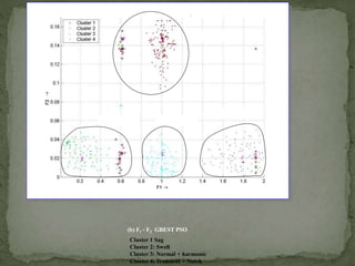
  • 33. (a) F1- F2 K-Means PSO Cluster-4 Cluster-3 Cluster-1 Cluster-2 HYBRID PSO OUTPUT : Cluster 1 Sag Cluster 2: Swell Cluster 3: Normal + harmonic Cluster 4: Transient + Notch
  • 34. GBEST PSO OUTPUT (b) F1 - F2 GBEST PSO Cluster-1 Cluster-4 Cluster-3Cluster-2 GBEST PSO OUTPUT Cluster 1 Sag Cluster 2: Swell Cluster 3: Normal + harmonic Cluster 4: Transient + Notch
  • 35. (c) F1- F2 GPAC APSO GPAC APSO OUTPUT Cluster-4 Cluster-1 Cluster-3 Cluster-2 Cluster 1 Sag Cluster 2: Swell Cluster 3: Normal + harmonic Cluster 4: Transient + Notch
  • 36. F1 - F2 Fitness Plots GPAC APSO PSO K-Means GBEST PSOGPAC APSO K-Means PSO GPAC-APSO GBEST PSO
  • 37. The proposed method is very efficient and simple to implement for clustering analysis when the number of clusters is known a priori. The modified GPAC-PSO known as GPAC-APSO is found to be more efficient and has a quick convergence property in comparison to other PSO variants.
  • 38. The next step in this research is to transform the visually distinguishable patterns to feature vectors that can be used by classifiers such as neural networks to automatically classify the disturbances.
  • 39. * In order to improve the classification accuracy a novel neural architecture comprising hybrid combinations of the radial basis function neural network and a functional link network that provides a more robust pattern recognizer for non-stationary time series data is undertaken for detailed study.
  • 40. Signal S-transform Feature extraction Neural Network Display recognized patterns PO ST PR OC ESS I NG A Neural network architecture is used to test the efficacy of the proposed method.
  • 41.   2 1   Q j ij xdE )()1( kEk w   where Q is the number of training samples and the weights are updated as where wE is the gradient with respect to weight, and  is the momentum constant, and  is the learning rate.
  • 42. It consists of a radial basis layer and a competitive layer. FIGURE 4.3 TO INSERT
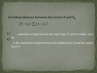
  • 43. where i number of input layers; h number of hidden layers j number of output layers; k number of training examples; Nk number of classification (clusters); σ smoothing parameters (standard deviation), 0.1< σ <1 X input vector; The algorithm of the inference output vector Y in the PNN is as follows: 1 . and ,hy hy j hj h j hj h hj net W H N W N    max( ) then 1, else 0j k j j k net net Y Y  If
  • 44. Euclidean distance between the vectors X and Xkj,   2 kj i kji X X X X   connection weight between the input layer X and the hidden layer H; is the connection weight between the hidden layer H and the output layer Y. xh ihW hy hjW
  • 45. We use RBFs with the random vector functional link nets (RVFLNs) to obtain the powerful radial basis functional link nets (RBFLNs). As RBFNN represents a nonlinear model while the RBFLN includes that nonlinear model as well as a linear model (the direct lines from the input to output nodes) so that the linear parts of a mapping do not need to be approximated by the nonlinear model.
  • 46. Radial Basis Functional Link Net (RBFLN)
  • 47. For an input vector , the output of th output node produced by an RBF is given by        11 11 )( 1 1 )( 2 )()()( m n noj m i i ctx ij m i m n nojiijj txwewtxwtwto i   where is the center of the ‘i’ th hidden node, is the width of the ‘i’th center, and is the total number of hidden nodes. If output of the hidden neurons, by vector notation ))t(....,),........t(),t(( tot 21 and weight vector for the hidden RBF units
  • 48. )w,......,w,w(w mjj2j1j  and the weight vector for the linear units )w,.......,w,w(w mjj2j1j  RBFLN output can be written as j T jj wwo  The sets of centers are trained with K-means clustering approach, where the centers are initially defined as the first training inputs that correspond to a specific class . The Centroid vector is given by  )c(x.,),........c(x),c(x)i(C mcc 210  c
  • 49. At each iteration , following a new input is presented, the distance for each of the centers is denoted by i )(ix )i(jj c)i(x)i( 1 cm...,,.........2,1j where The kth center is updated by the following equation: )i()i(C)i(C kkk  1 k is chosen in such a way that it minimizes )(ij )i(arg(min(k jThus and is the learning rate.
  • 50. The width associated with the k th center is adjusted as 2 1 1   aN j jkk )i(C)i(C N )i( Where N is the number of hidden neurons. Wavelet based Neural Classification Schemes Method-1 (WT-1) was implemented using the thirteen level coiflet 5-wavelet decomposition. The de-noising step in Method-2(WT-2) was omitted to test its effectiveness in noise. A hybrid DFT-DWT fuzzy expert system approach known as Method-3 (WT-3) is also considered in this paper for feature extraction and disturbance pattern classification.
  • 52. Block diagram of classification algorithm
  • 53. The important features obtained from the Fourier (DFT) and wavelet analysis (DWT) for the non-stationary disturbance time series data are listed as follows: 1 Fundamental and harmonic components obtained from the Discrete Fourier Transform of the time series signal data samples. 2. The phase angle shift of the disturbance time series with respect to normal waveform Ln. 3. Number of peaks of the wavelet coefficients (Nn). 4. Energy of the wavelet coefficients (Ewn). 5. Oscillation number of missing voltage time series data.
  • 54. The extracted features are then used with different types of neural classifiers such as multilayered perceptron network, probabilistic neural network, and proposed radial basis functional link network for pattern classification, data mining and subsequent knowledge discovery.
  • 55. MLP Pure 30dB Method WT-1 WT-2 ST WT-1 WT-2 ST Oscillatory transient 95% 95% 90% 30% 90% 95% Impulsive transient 100% 70% 95% 100% 65% 85% Multiple notch 100% 85% 100% 90% 85% 100% Voltage swell 100% 100% 100% 55% 95% 100% Voltage sag 90% 80% 80% 60% 85% 96% Interruption 100% 90% 100% 100% 95% 100% Harmonics 100% 85% 90% 15% 80% 85% Swell + harmonics 100% 95% 100% 60% 95% 100% Sag +harmonics 100% 80% 100% 25% 80% 100% Average 98.33% 86.67% 95% 59.44% 85.56% %
  • 56. RBFLN Pure 30dB Method WT-1 WT-2 ST WT-1 WT-2 ST Oscillatory transient 95% 95% 80% 45% 30% 90% Impulsive transient 100% 75% 100% 95% 65% 70% Multiple notch 85% 85% 90% 85% 85% 95% Voltage swell 100% 95% 90% 75% 95% 90% Voltage sag 85% 85% 80% 80% 85% 70% Interruption 100% 100% 100% 25% 100% 100% Harmonics 100% 95% 90% 5% 80% 90% Swell +harmonics 100% 100% 100% 50% 100% 100% Sag+harmonics 80% 85% 100% 55% 85% 100%
  • 57. Method WT-1 WT-2 ST WT-1 WT-2 ST Oscillatory transient 95% 95% 95% 35% 15% 80% Impulsive transient 100% 65% 95% 100% 70% 60% Multiple notch 100% 85% 90% 90% 90% 95% Voltage swell 100% 100% 90% 50% 100% 85% Voltage sag 75% 85% 80% 35% 85% 75% Interruption 100% 100% 100% 100% 100% 100% Harmonics 95% 90% 90% 25% 85% 90% Swell+ harmonics 85% 100% 100% 45% 100% 100% Sag+harmonics 60% 80% 75% 45% 75% 70% Average 90% 88.89% 90.56% 58.33% 80% 83.89%
  • 58. Type of time series data Number of disturbances Number of class correctly identified WT-3 ST Sag 100 99 92 Swell 100 100 96 Interruption 100 100 97 Harmonics 100 98 95 Switching transients 100 95 90 Impulse 100 92 97 Flicker 100 99 96 Notch 100 100 94 Average 100% 97.87% 94.62%