module1_Introductiontoalgorithms_2022.pdf

MODULE 1
INTRODUCTION TO
ALGORITHM ANALYSIS

2
What is an algorithm?
An algorithm is
a sequence of unambiguous instructions
for solving a computational problem,
i.e., for obtaining a required output
for any legitimate input
in a finite amount of time.
Shiwani Gupta

4
Features of Algorithm
• Input : zero or more valid inputs are clearly specified
• Output: produce at least 1 correct output given valid input
• Definiteness: clearly and unambiguously specified
instructions
• Finiteness : terminates after finite steps for all cases
• Effectiveness: steps are sufficiently simple and basic
Shiwani Gupta

5
A Brief History of Algorithms
• According to the Oxford English Dictionary, the
word algorithm is a combination of the Middle
English word algorism with arithmetic.
• The word algorism derives from the name of Arabic
mathematician Al-Khwarizmi.
• Al-Khwarizmi wrote a book on solving equations
from whose title the word algebra derives.
• It is commonly believed that the first algorithm was
Euclid’s Algorithm for finding the greatest common
divisor of two integers, m and n (m ≥n).
Shiwani Gupta

6
Rules for writing a Pseudocode
• Head
Algorithm name (<parameter list>)
//Problem Description:
// Input:
// Output:
• Body {includes programming constructs or assignment statements}
Compound statements enclosed in { }
Single line comments //
Identifier can be combination of alphanumeric string beginning by letter
Use assignment operator
Boolean, Logical, Relational operators
Array indices [ ] begin with 0
Input and Output using read(val) and write(“Hello”)
if (condition) then statement
if (condition) then statement else statement
Shiwani Gupta

7
while (cond) do
{
stmt 1
stmt 2
:
:
stmt n
}
for var val1 to valn do
{
stmt 1
stmt 2
:
:
stmt n
}
Rules for writing a Pseudocode
repeat
{
stmt 1
stmt 2
:
:
stmt n
} until (condition)
break stmt to exit from inner loop
return stmt to return control from one
point to another
Shiwani Gupta

8
• Brute Force
• Divide and Conquer / Decrease and Conquer
– Merge Sort / Binary Search
• Greedy Method
– Kruskal algorithm for Minimal Spanning Tree
• Dynamic Programming
– All Pair Shortest Path
• Search and Enumeration (Search algo, B&B,
Backtracking)
– Graph Problems
• Probabilistic and Heuristics and Genetic
Classification by Design Paradigm
Shiwani Gupta

9
Classification of Algorithm by Implementation
• Recursion / Iteration
– Tower of Hanoi, Fibonacci
• Logical
– Algorithm = logic + control
• Serial / Parallel or Distributed
– Sorting, Iterative
• Deterministic / Non Deterministic
– Exact decision / Guess via heuristics
• Exact / Approximate
– Approximate algorithms are useful for hard problems
Shiwani Gupta

10
Performance Analysis of Algorithm
• Determine run-time of a program as function of
input –TIME COMPLEXITY
• Determine total or maximum memory required for
program data – SPACE COMPLEXITY
• Determine total size of program code
• Determine whether program correctly computes
desired result
• Determine complexity of program
– Ease of reading, understanding and modification
• Determine robustness of program
– Dealing with unexpected and erroneous input
Shiwani Gupta

11
Space Complexity
• The space S(p) needed by an algorithm is the sum of
a fixed part and a variable part
• The fixed part c includes space for
– Instructions
– Variables
– Identifiers
– Constants
• The variable part Sp includes space for
– Variables whose size is dependant on the particular
problem instance being solved
– Recursion stack space S(p) = c + Sp
Shiwani Gupta

12
Algorithm abc (a, b, c)
{
return a+b+b*c+((a+b-c)/(a+b)+4.0
}
For every instance 3 computer words require to store variables: a, b, c
Sp () = 3
Shiwani Gupta

13
Algorithm Sum (a, n)
{
s:=0.0
for i 1 to n do
s = s + a[i]
return s
}
Every instance needs to store array a[] and n
Space needed to store n = 1 word
Space needed to store a[] = n floating point words
Space needed to store i and s = 2 words
Sp (n) = n+3
Shiwani Gupta

14
Time Complexity
• The time complexity of a problem is
– The number of steps that it takes to solve an instance of
the problem as a function of the size of the input (usually
measured in bits), using the most efficient algorithm.
• The time needed by an algorithm T(p) is the sum of
a fixed part and a variable part
– The fixed part includes compile time c which is
independent of problem instance.
– The variable part is the run time tp which is dependent on
problem instance.
T(p) = c + tp
Shiwani Gupta

15
Analyzing Running Time
1. read(n)
2. Sum ← 0
3. i ← 0
4. while (i < n) do
5. read(number)
6. sum ← sum + number
7. i ← i + 1
8. mean ← sum / n
T(n), or the running time of a particular algorithm on input of size n, is
taken to be the number of times the instructions in the algorithm are
executed.
Example pseudo code illustrates the calculation of the mean (average) of
a set of n numbers:
Number of times executed
1
1
1
n+1
n
n
n
1
The computing time for this algorithm in
terms on input size n is: T(n) = 4n + 5.

16
Sr.
No.
Statements S/E Freq. Total
1 Algorithm Sum(a, n ) 0 - 0
2 { 0 - 0
3 s←0.0 1 1 1
4 for i ← 1 to n do 1 n+1 n+1
5 s←s+a[i] 1 n n
6 return s 1 1 1
7 } 0 - 0
Shiwani Gupta

17
Sr.
No.
1 Algorithm Add(a, b, c, n, m ) 0 - 0
2 { 0 - 0
3 for i ←1 to n do 1 n+1 n+1
4 for j ← 1 to m do 1 n(m+1) n(m+1)
5 c[i,j] ← a[i,j]+b[i,j] 1 nm nm
6 } 0 - 0
Shiwani Gupta

18
Sr.
No.
n=
0
n>
0
n=
0
n>0
1 Algorithm RSum(a, n ) 0 - - 0 0
2 { 0 0 0 - -
3 if(n<=0) then 1 1 1 1 1
4 return 0.0 1 1 0 1 0
5 else return Rsum(a,n-1)+a[n] 1+tRsum(n-1) 0 1 0 1+tRsum(n-1)
6 } 0 0 0 - -
Shiwani Gupta

19
Best, average, worst-case Efficiency
• Worst case:
– Efficiency (# of times the basic operation will be executed) for the worst case
input of size n, for which
– The algorithm runs the longest among all possible inputs of size n.
• Best case:
– Efficiency (# of times the basic operation will be executed) for the best case
input of size n, for which
– The algorithm runs the fastest among all possible inputs of size n.
• Average case:
– Efficiency (#of times the basic operation will be executed) for a typical/random
input
– NOT the average of worst and best case.
Shiwani Gupta

20
Growth of function (Asymptotics)
Used to formalize that an algorithm has running
time or storage requirements that are
``never more than'' ,
``always greater than” , or
``exactly'' some amount
Less than equal to (“≤”)
Greater than equal to (“≥”)
Equal to (“=“)
Shiwani Gupta

21
Big Oh (O) Notation
Asymptotic Upper Bound
Definition 1: Let f(n) and g(n) be two functions. We write:
f(n) = O(g(n)) or f = O(g)
(read "f of n is big oh of g of n" or "f is big oh of g")
if there is a positive integer c such that f(n) <= c * g(n) for all positive integers n>n0.
The basic idea of big-Oh notation is this: Suppose f and g are both real-valued functions
of a real variable x. If, for large values of x, the graph of f lies closer to the horizontal
axis than the graph of some multiple of g, then f is of order g, i.e., f(x) = O(g(x)). So,
g(x) represents an upper bound on f(x).
Shiwani Gupta

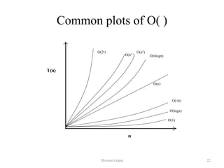
22
Common plots of O( )
O(2n)
O(n3 )
O(n2)
O(nlogn)
O(n)
O(√n)
O(logn)
O(1)
Shiwani Gupta

23
Omega (Ω) Notation
Asymptotic Lower Bound
f(n) = Ω(g(n)) or f = Ω(g)
(read "f of n is omega of g of n" or "f is omega of g")
if there is a positive integer c such that f(n) >= c * g(n) >= 0 for all positive integers n>n0.
The basic idea of omega notation is this: Suppose f and g are both real-valued functions
of a real variable x. If, for large values of x, the graph of some multiple of g lies closer
to the horizontal axis than the graph of f, then f is of order g, i.e., f(x) = Ω(g(x)). So,
g(x) represents an lower bound on f(x).
Shiwani Gupta

24
Theta (Θ) Notation
Asymptotic Tight Bound
f(n) = Θ (g(n)) or f = Θ (g)
(read "f of n is theta of g of n" or "f is theta of g")
if there is a positive integer c such that
c2 * g(n) >= f(n) >= c1 * g(n) >= 0 for all positive integers n.
The basic idea of theta notation is this: Suppose f and g are both real-valued functions
of a real variable x. If, for large values of x, the graph of some multiple of g lies closer
to the horizontal axis than the graph of f and the graph of f lies closer to the horizontal
axis than some other multiple of g, then f is of order g, i.e., f(x) = Ω(g(x)). So, g(x)
represents a tight bound on f(x). Thus g(x) is both upper and lower bound on f(n).
Thus, (f) = O(f)  (f)
Shiwani Gupta

25
Compare n and (n+1)/2
lim( n / ((n+1)/2 )) = 2,
same rate of growth
(n+1)/2 = Θ(n)
rate of growth of a linear function
Compare n2 and n2+ 6n
lim( n2 / (n2+ 6n ) )= 1
same rate of growth.
n2+6n = Θ(n2)
rate of growth of a quadratic function
Compare log n and log n2
lim( log n / log n2 ) = 1/2
same rate of growth.
log n2 = Θ(log n)
logarithmic rate of growth
Θ(n3): n3
5n3+ 4n
105n3+ 4n2 + 6n
Θ(n2): n2
5n2+ 4n + 6
n2 + 5
Θ(log n): log n
log n2
log (n + n3)
Shiwani Gupta

26
Input
Size:
n
(1) log n n n log n n² n³ 2ⁿ n!
constant log linear n-log-n quadratic cubic exponential factorial
Scanning
Array
Elements
Performing
Binary
Search
Operation
Performing
Sequential
Search
Operation
Sorting
Elements
using Merge
Sort or Quick
Sort
Scanning
Matrix
Elements
Performing
Matrix
Multiplicatio
n
Towers of
Hanoi
problem
Traveling
Salesman
Problem by
Brute Force
Search
5 1 3 5 15 25 125 32 120
10 1 4 10 33 100 10³ 10³ 3628800
100 1 7 100 664 104 106 1030 9.33e+157
1000 1 10 1000 104 106 109 10300 4.02e+2567
10000 1 13 10000 105 108 1012 103000 2.84e+35659
Generalizing Running Time (Basic Efficiency classes)
Shiwani Gupta

27
Running Time Calculations - Loops
for (j = 0; j < n; ++j) {
// 3 atomics
}
• Complexity = (3n) = (n)
- Loops with Break
for (j = 0; j < n; ++j) {
// 3 atomics
if (condition) break;
}
• Upper bound = O(4n) = O(n)
• Lower bound = (4) = (1)
• Complexity = O(n)
Shiwani Gupta

28
- Loops in
Sequence
for (j = 0; j < n; ++j) {
// 3 atomics
}
for (j = 0; j < n; ++j) {
// 5 atomics
}
• Complexity = (3n + 5n) = (n)
- Nested
Loops
for (j = 0; j < n; ++j) {
// 2 atomics
for (k = 0; k < n; ++k) {
// 3 atomics
}
}
• Complexity = ((2 + 3n)n) = (n2)
Shiwani Gupta

29
-Multiply
Loop
1 i=1
2 loop (i<n)
1 appl code
2 i = i*2
Complexity = (3log2 n + 2) = (log2 n)
- Divide
Loop
Logarithmic Loops
1 i=n
2 loop (i>=1)
1 appl code
2 i = i/2
Complexity = (3log2 n + 5) = (log2 n)
Shiwani Gupta

30
-Dependent
Quadratic
1 i=1
2 loop (i<=n)
1 j=1
2 loop (j<=i)
1 appl code
2 j=j+1
3 i=i+1
Complexity = ((3n(n+1)/2)+3n+3) = (n2)
- Quadratic
1 i=1
2 loop (i<=n)
1 j=1
2 loop (j<=n)
1 appl code
2 j=j+1
3 i=i+1
Complexity = ((3n2+4n+2) = (n2)
Shiwani Gupta

31
- Consecutive
Statements
for (i = 0; i < n; ++i) {
// 1 atomic
if(condition) break;
}
for (j = 0; j < n; ++j) {
// 1 atomic
for (k = 0; k < n; ++k) {
// 3 atomics
}
}
• Complexity =
O(2n) + O((3+3n)n)
• = O(n) + O(n2) = ??
• = O(n2)
Shiwani Gupta

32
1 i=1
2 loop (i<=n)
1 j=1
2 loop (j<n)
1 appl code
2 j=j*2
3 i=i+1
Complexity = (4n+3nlogn+1) = (nlogn)
- Linear Logarithmic
Shiwani Gupta

33
- If-then-else
if(condition)
i = 0;
else
for ( j = 0; j < n; j++)
a[j] = j;
• Complexity
= O(1) + max ( O(1), O(N))
= O(1) + O(n)
= O(n)
- Sequential Search
• Given an unsorted vector a[], find if the element X occurs in a[]
for (i = 0; i < n; i++) {
if (a[i] == X) return true;
}
return false;
• Complexity = O(n)
Shiwani Gupta

34
Mathematical Background for non
recursive algorithm analysis
1. Decide on a parameter(s) indicating an input’s size.
2. Identify algorithm’s basic operation.
3. Check whether the number of times basic operation is executed
depends only on size of input.
4. Investigate worst, average and best case efficiencies.
5. Find no. of times basic operation is executed.
6. Either Find a closed formula for count OR It’s order of growth.
// Largest element in an array
ALGORITHM
MaxElement(A[0...n-1])
Maxval A[0]
for i 1 to n-1 do
if A[i]>maxval
maxval A[i]
return maxval Shiwani Gupta

35
Mathematical Background for recursive
algorithm analysis
1. Decide on a parameter(s) indicating an input’s size.
2. Identify algorithm’s basic operation.
3. Check whether the number of times basic operation is executed can
vary on different inputs of same size.
4. Investigate worst, average and best case efficiencies.
5. Set up a recurrence relation with an appropriate initial condition for
no. of times the basic operation is executed.
6. Solve recurrence or ascertain order of growth.
// factorial for an arbitrary nonnegative no.
ALGORITHM F(n)
if n=0 return 1
else return F(n-1)*n
Shiwani Gupta

36
Algorithm: Fibonacci
Algorithm 1 fib(n)
if n = 0 then
return (0)
if n = 1 then
return (1)
return (fib(n − 1) + fib(n − 2))
Algorithm 2: fib(n)
comment: Initially we create an array A[0: n]
A[0] ← 0, A[1] ← 1
for i = 2 to n do
A[i] = A[i − 1] + A[i − 2]
return (A[n])
Recurrence Relation of Fibonacci Number fib(n):
{0, 1, 2, 3, 5, 8, 13, 21, 34, 55, 89, 144, 233, …}
Shiwani Gupta

TASK
• Determine the running time of a piece of code for the following cases:
(i) Dependent loop (ii) If-then-else statement (iii) Nested For loop
• An algorithm takes 0.5ms for input size 100. How long will it take for input
size 500 if run time is
(i) quadratic (ii) nlogn
• Calculate the running time for following program segment.
i=1
loop(i<=n)
print(i)
i=i+1
• Write procedure to find sum of series and find time complexity.
• Write a routine for finding factorial of a given number using recursion.
• Define notations. State their interrelationship.
Shiwani Gupta 37

Selection Sort
• Task: rearrange books on shelf by height
– Shortest book on the left
• Approach:
– Look at books, select shortest book
– Swap with first book
– Look at remaining books, select shortest
– Swap with second book
– Repeat …
Shiwani Gupta 38

Selection Sort
A selection sort of an array of integers into
ascending order.
Shiwani Gupta 39

Iterative Selection Sort
Algorithm selectionSort(a, n)
// Sorts the first n elements of an array a.
for (index = 0; index < n - 1; index++)
{ indexOfNextSmallest = the index of the smallest value among
a[index], a[index+1], . . . , a[n-1]
Interchange the values of a[index] and a[indexOfNextSmallest]
// Assertion: a[0] £ a[1] £ . . . £ a[index], and these are the smallest of
the original array elements.
// The remaining array elements begin at a[index+1].
}
Shiwani Gupta 40

Recursive Selection Sort
Algorithm selectionSort(a, first, last)
// Sorts the array elements a[first] through a[last] recursively
if (first < last)
{ indexOfNextSmallest = the index of the smallest value among
a[first], a[first+1], . . . , a[last]
Interchange the values of a[first] and a[indexOfNextSmallest]
// Assertion: a[0] £ a[1] £ . . . £ a[first] and these are the smallest of
the original array elements.
// The remaining array elements begin at a[first+1].
selectionSort(a, first+1, last)
}
Shiwani Gupta 41

The Efficiency of Selection Sort
• Iterative method for loop executes n – 1 times
– For each of n – 1 calls, the indexOfSmallest is invoked, last is n-1,
and first ranges from 0 to n-2.
– For each indexOfSmallest, compares last – first times
– Total operations: (n – 1) + (n – 2) + …+ 1 = n(n – 1)/2 = O(n2)
• It does not depends on the nature of the data in the array.
• Recursive selection sort performs same operations
– Also O(n2)
Shiwani Gupta 42

Insertion Sort
• If only one book, it is sorted.
• Consider the second book, if shorter than first one
– Remove second book
– Slide first book to right
– Insert removed book into first slot
• Then look at third book, if it is shorter than 2nd book
– Remove 3rd book
– Slide 2nd book to right
– Compare with the 1st book, if is taller than 3rd, slide 1st to right,
insert the 3rd book into first slot
Shiwani Gupta 43

Insertion Sort
• Partitions the array into two parts. One part is sorted and initially
contains the first element.
• The second part contains the remaining elements.
• Removes the first element from the unsorted part and inserts it into
its proper sorted position within the sorted part by comparing with
element from the end of sorted part and toward its beginning.
• The sorted part keeps expanding and unsorted part keeps shrinking
by one element at each pass
Shiwani Gupta 44

Insertion Sort
at each iteration, the array is divided in two sub-arrays:
Shiwani Gupta 45

INSERTION-SORT (Iterative)
Alg.: INSERTION-SORT(A)
for j ← 2 to n
do key ← A[ j ]
Insert A[ j ] into the sorted sequence A[1 . . j -1]
i ← j - 1
while i > 0 and A[i] > key
do A[i + 1] ← A[i]
i ← i – 1
A[i + 1] ← key
a8
a7
a6
a5
a4
a3
a2
a1
1 2 3 4 5 6 7 8
key
Shiwani Gupta 46

Analysis of Insertion Sort
cost times
c1 n
c2 n-1
0 n-1
c4 n-1
c5
c6
c7
c8 n-1
 
n
j j
t
2
 

n
j j
t
2
)
1
(
 

n
j j
t
2
)
1
(
    )
1
(
1
1
)
1
(
)
1
(
)
( 8
2
7
2
6
2
5
4
2
1 










 

 


n
c
t
c
t
c
t
c
n
c
n
c
n
c
n
T
n
j
j
n
j
j
n
j
j
INSERTION-SORT(A)
for j ← 2 to n
do key ← A[ j ]
Insert A[ j ] into the sorted sequence A[1 . . j -1]
i ← j - 1
while i > 0 and A[i] > key
do A[i + 1] ← A[i]
i ← i – 1
A[i + 1] ← key
tj: # of times the while statement is executed at iteration j
 n2/2 comparisons
 n2/2 exchanges
Shiwani Gupta 47

Best Case Analysis
• The array is already sorted
– A[i] ≤ key upon the first time the while loop test is run
(when i = j -1)
– tj = 1
• T(n) = c1n + c2(n -1) + c4(n -1) + c5(n -1) + c8(n-1)
= (c1 + c2 + c4 + c5 + c8)n + (c2 + c4 + c5 + c8)
= an + b a linear function of n
T(n) = (n) linear growth
“while i > 0 and A[i] > key”
Shiwani Gupta 48

Worst Case Analysis
• The array is in reverse sorted order
– Always A[i] > key in while loop test
– Have to compare key with all elements to the left of the j-th
position  compare with j-1 elements  tj = j
a quadratic function of n
T(n) = (n2) quadratic growth
1 2 2
( 1) ( 1) ( 1)
1 ( 1)
2 2 2
n n n
j j j
n n n n n n
j j j
  
  
      
  
)
1
(
2
)
1
(
2
)
1
(
1
2
)
1
(
)
1
(
)
1
(
)
( 8
7
6
5
4
2
1 


















 n
c
n
n
c
n
n
c
n
n
c
n
c
n
c
n
c
n
T
c
bn
an 

 2
“while i > 0 and A[i] > key”
using we have:
Shiwani Gupta 49

Recursive Insertion Sort
Algorithm insertionSort(a, first, last)
// Sorts the array elements a[first] through a[last] recursively.
if (the array contains more than one element)
{ Sort the array elements a[first] through a[last-1]
Insert the last element a[last] into its correct sorted position
within the rest of the array
}
• Complexity is O(n2).
• Usually implemented nonrecursively.
• If array is closer to sorted order; Less work the insertion sort does
and hence more efficient the sort is
• Insertion sort is acceptable for small array sizes
Shiwani Gupta 50

Recurrence Relations
• Equation or an inequality that characterizes a function by its
values on smaller inputs.
• Solution Methods
– Substitution Method.
– Recursion-tree Method.
– Master Method.
• Recurrence relations arise when we analyze the running
time of iterative or recursive algorithms.
– Ex: Divide and Conquer.
T(n) = (1) if n  d
T(n) = a T(n/b) + D(n) + C(n) otherwise
Shiwani Gupta 51

Substitution Method
• Guess the form of the solution, then
use mathematical induction to show it correct.
– Substitute guessed answer for the function when the inductive
hypothesis is applied to smaller values – hence, the name.
• Works well when the solution is easy to guess.
• No general way to guess the correct solution.
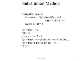
Shiwani Gupta 52

Shiwani Gupta 53
T(n)=T(n−1)+c1
T(1)=c2
assume c1 = c2 = 1
T(n)=T(n−1)+1=(T(n−2)+1)+1=T(n−2)+2...
T(n)=T(n-(n-1))+(n-1)=T(1)+(n-1)
T(n)=n
Example: Factorial
Recurrence: F(n)=F(n-1)*n , n>0
M(n) = M(n-1) + 1
Guess: M(n) = n
Substitution Method

Tower of Hanoi
A mathematical puzzle where we have three rods and n
disks.
The objective of the puzzle is to move the entire stack to
another rod, obeying the following simple rules:
1) Only one disk can be moved at a time.
2) Each move consists of taking the upper disk from one
of the stacks and placing it on top of another stack i.e. a
disk can only be moved if it is the uppermost disk on a
stack.
3) No disk may be placed on top of a smaller disk.
Shiwani Gupta 54

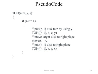
Shiwani Gupta 56
PseudoCode
TOH(n, x, y, z)
{
if (n >= 1)
{
// put (n-1) disk to z by using y
TOH((n-1), x, z, y)
// move larger disk to right place
move:x-->y
// put (n-1) disk to right place
TOH((n-1), z, y, x)
}
}

Analysis
Shiwani Gupta 57
Recursive Equation : Eq-1
Solving it by Backsubstitution :
Eq-2
T(n-2) = 2T(n-3) + 1 Eq-3
Put the value of T(n-2) in the Eq-2 with help of Eq-3
Eq-4
Put the value of T(n-1) in Eq-1 with help of Eq-4
After Generalization :
Base condition T(1) =1
n – k = 1
k = n-1
put, k = n-1
It is a GP series, and the sum is
or you can say which is exponential

Recursion-tree Method
• Making a good guess is sometimes difficult with the
substitution method.
• Use recursion trees to devise good guesses.
• Recursion Trees
– Show successive expansions of recurrences using trees.
– Keep track of the time spent on the subproblems of a
Divide and Conquer algorithm.
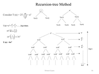
Shiwani Gupta 58

Shiwani Gupta 59
Consider T (n) = 2T + n2
Recursion-tree Method

Master Method
• Many Divide-and-Conquer recurrence equations have the form:
where a>=1, b>1, f(n) is asymptotically positive function
• The Master Theorem Cases:







d
n
n
f
b
n
aT
d
n
c
n
T
if
)
(
)
/
(
if
)
(
log log
log log 1
log
1. if ( ) is ( ), then ( ) is ( ), 0
2. if ( ) is ( log ), then ( ) is ( log )
3. if ( ) is ( ), then ( ) is ( ( )), 0
provided ( / ) ( ) for some 1.
b b
b b
b
a a
a a
k k
a
f n O n T n n
f n n n T n n n
f n n T n f n
af n b f n




 



 
 
  
 
f(n) grows asymptotically slower
Same growth rate
f(n) grows asymptotically faster
Compare f(n) and nlog
b
a
Requires memorization of three cases
60

Master Method
Eg. 1:
Eg. 2:
Eg. 3:
Eg. 4:
Eg. 5:
Eg. 6:
n
n
T
n
T 
 )
2
/
(
4
)
(
Solution: logba=2, so case 1 says T(n) is Ѳ(n2).
n
n
n
T
n
T log
)
2
/
(
2
)
( 

Solution: logba=1, so case 2 says T(n) is Ѳ(n log2 n).
n
n
n
T
n
T log
)
3
/
(
)
( 

Solution: logba=0, so case 3 says T(n) is Ѳ(n log n) , (δ=1/3<1).
n
n
T
n
T log
)
2
/
(
2
)
( 

Solution: logba=1, so case 1 says T(n) is Ѳ(n).
1
)
2
/
(
)
( 
 n
T
n
T
Solution: logba=0, so case 2 says T(n) is Ѳ(log n).
3
)
3
/
(
9
)
( n
n
T
n
T 

Solution: logba=2, so case 3 says T(n) is Ѳ(n3) , (1/3<δ=1/3<1).
Heap construction
Binary search
61

Task
• Explain the terms in the recurrence relation: T(n)= aT(n/b) + f(n)
• Explain Master's Method for solving recurrences to obtain asymptotic bounds.
• Solve the recurrence using Master Method -
a. T(n) = 16T (n/4) + n
b. T(n) = 3T (n/4) + n log n
c. T(n) = 2T (n/4) + √n
d. T(n) = 4T (n/2) +n2
e. T(n) = 2T (n/2) +n3
f. T(n) = 16T (n/4) +n2
• Arrange the following functions in increasing order. n, logn, n3, n2, nlogn, 2n, n!
• Frame and solve the recurrence using Substitution method for –
a. Tower of Hanoi b Fibonacci series c Factorial
• Solve using recursion tree method
a. T(n) = 3T(n/4)+n2
b. T(n) = 2T(n/2)+n2
62
g. T(n) = 16T(n/4) - n2log n
h. T(n) = 2T(n/2) + n, n>1
i. T(n) = T(n/2)+1
j. T(n) = 9T(n/3)+n
k. T(n) = 3T (n/2) +n
l. T(n) = 64T (n/4) + n
c. T(n) = 3T(n/2)+cn2
d. T(n) = T(n/3)+T(2n/3)+n
e. T(n) = 3T (n/2) +n

module1_Introductiontoalgorithms_2022.pdf

Recommended

More Related Content

Similar to module1_Introductiontoalgorithms_2022.pdf (20)

More from Shiwani Gupta (20)

Recently uploaded (20)

module1_Introductiontoalgorithms_2022.pdf