Monte-Carlo method for Two-Stage SLP

Lecture 5

Monte-Carlo method for Two-Stage
SLP
Leonidas Sakalauskas
Institute of Mathematics and Informatics
Vilnius, Lithuania <sakal@ktl.mii.lt>

EURO Working Group on Continuous Optimization

Content
 Introduction
 Monte Carlo estimators

 Stochastic Differentiation

  -feasible gradient approach for two-stage SLP

 Interior-point method for two stage SLP

 Testing optimality

 Convergence analysis

 Counterexample

Two-stage stochastic optimization
problem

 
F ( x)  c  x  E min y [q  y | W  y  T  x  h, y  R ]  min
m

Ax  b, x  n ,


assume vectors q, h and matrices W, T random in
general.

problem

 Say, vector h can be distributed
multivariate normally:
N ( , S )

here  , S are correspondingly the
vector of means and the covariance
matrix

problem

the random vector Z distributed with
respect to N (  , S ) is simulated as

Z  R
T

 is standard normal vector,
R is triangle matrix that

RT  R  S
(Choletzky factorization)

Two-stage stochastic optimization problem with
complete recourse will be

F ( x )  c  x  E Q ( x,  )  min n
xD 

subject to the feasible set


D  x A  x  b, x  R
n

where

Q( x,  )  min y [q  y | W  y  T  x  h, y  R ]
m

It can be derived under the assumption on the existence
of a solution at the second stage and continuity of
measure P, that the objective function is smoothly
differentiable and the gradient is

 x F ( x)  Eg ( x,  )
where

g ( x,  )  c  T  u *

is given by the set of solutions of the dual problem

(h  T  x)T  u *  max u [(h  T  x)T  u | u  W T  q  0, u  R ]
s

Monte-Carlo samples
We assume here that the Monte-Carlo sample of a
certain size N is provided for any x  D  n

Y  ( y1, y 2 ,..., y N ),
the sampling estimator of the objective function

1 N
F ( x)   f ( x, y )
j

N j 1
and sampling variance can be computed
1 N
  
2
D ( x) 
2
f ( x, y j )  F ( x)
N  1 j 1

Gradient

The gradient is evaluated using
the same random sample:

1 N
g ( x)   g ( x, y ),
j

N j 1
xD  R n

Covariance matrix

We use the sampling covariance matrix

1 N
 
 g  x, y   g  x   g  x, y   g  x  
T
A( x)  j j

N  n j 1

later on for normalising the gradient estimator.

 – feasible direction approach

Let us define the set of feasible
directions as follows:

 
V ( x)  g  Ag  0, 1in  g j  0, if x j  0 
n

Gradient projection

Denote, gU as projection of vector g onto the set U.
Since the objective function is differentiable, the
solution
xD
is optimal if
F  x V  0

Gradient projection

the projection of G onto the set
Ax  0
is
GA  G  P
T


P  I  A  A A
T T 1
 A

where is projector

Assume a certain multiplier 0 to be given.
Define the function  : V ( x)   
x
by
 
1 j n g j  0
 xj 
 x ( g )  min   , min( ) 
ˆ
 1j 0, g j 
g
 j n 

Thus, x    g  D , when    x ( g ),
for any g V  x  , x  D

Now, let a certain small value   0 be given.

Then we introduce the function  x : V ( x)  
 x ( g )    maxmin x j ,   g j  ,
ˆ ˆ  g  0 ,
1 j  n
1 j  n j
g j 0

 x ( g )  0 , if 1 j  n ( g j  0)

and define the ε - feasible set

 
V ( x)  g n Ag  0, 1i n g j  0, if  0  x j   x ( g )  

The starting point can be obtained as the solution of the
deterministic linear problem:
( x 0 , y 0 )  arg min[c  x  q  y | A  x  b, W  y  T  x  h, y  R , x  R ].
m n
x, y

The iterative stochastic procedure of gradient search could
be used further:
xt 1  xt   t  G ( xt )
where  t   t (Gt ) is the step-length multiplier and
x
G  G( xt )
t
 -feasible the projection of gradient
estimator to the ε
 is set.
V xt

Monte-Carlo sample size problem

There is no a great necessity to compute
estimators with a high accuracy on starting the
optimisation, because then it suffices only to
approximately evaluate the direction leading to
the optimum.
Therefore, one can obtain not so large samples at
the beginning of the optimum search and, later
on, increase the size of samples so as to get the
estimate of the objective function with a desired
accuracy just at the time of decision making on
finding the solution to the optimisation problem.

We propose a following version for regulating the
sample size:

  n  Fish( , nt , N t  nt )   
N  min  max 
t 1
~ t T ~ t   n t ,N min ,N max 
    (G( x )  ( A( x t ))1  (G( x )  
   t   

Statistical testing of the optimality
hypothesis
The optimality hypothesis could be accepted for some
point x t with significance 1   , if the following
condition is sattisfied
~ ~
( N t  nt )  ( g ( x t ))T  A( x t ) 1  g ( x t )
T2   Fish(  , nt , N t  nt )
nt
Next, we can use the asymptotic normality again and
decide that the objective function is estimated with a
permissible accuracy  , if its confidence bound does
not exceed this value:
~ t
   D( x ) / N  
t

Computer simulation
 Two-stage stochastic linear optimisation problem.
 Dimensions of the task are as follows:
 the first stage has 10 rows and 20 variables;
 the second stage has 20 rows and 30 variables.

http://www.math.bme.hu/~deak/twostage/ l1/20x20.1/
(2006-01-20).

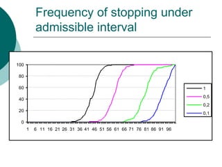
Two stage stochastic
programing

 The estimate of the optimal value of the objective
function given in the database is 182.94234  0.066
 N0=Nmin=100 Nmax=10000.
 Maximal number of iterations tmax  100 , generation of
trials was broken when the estimated confidence
interval of the objective function exceeds admissible
value  .
 Initial data were as follows:
 = =0.95;   0.99,   0.1; 0.2; 0.5; 1.0.

Frequency of stopping under
admissible interval

100

80

60 1
0,5
40
0,2
20
0,1

0
1 6 11 16 21 26 31 36 41 46 51 56 61 66 71 76 81 86 91 96

Change of the objective function
under admissible interval

184,5
184 0,1
183,5 0,2
183 0,5
182,5 1

182
1 12 23 34 45 56 67 78 89 100

Change of confidence interval
under admissible interval

7
6
5 0,1
4 0,2
3 0,5
2
1
1
0
1 8 15 22 29 36 43 50 57 64 71 78 85 92 99

Change of the Monte-Carlo sample
size under admissible interval

1400000
1200000
1000000 0,1
800000 0,2
600000 0,5
400000 1
200000
0
1 6 11 16 21 26 31 36 41 46 51 56 61 66 71 76 81 86 91 96

Hotelling statistics under
admissible interval
10
9
8
7 0,1
6
0,2
5
4 0,5
3 1
2
1
0
1 11 21 31 41 51 61 71 81 91

t
Nj
Histogram of ratio  Nt
j 1
under
admissible interval
30

25

20
0,1
0,2
15
0,5
1
10

5

0
8 10 12 14 16 18 20 22 24 26 28 30 32 34 36

Wrap-Up and Conclisions
 The stochastic adaptive method has been developed to
solve stochastic linear problems by a finite sequence of
Monte-Carlo sampling estimators

 The method is grounded by adaptive regulation of the size
of Monte-Carlo samples and the statistical termination
procedure, taking into consideration the statistical
modeling accuracy

 The proposed adjustment of sample size, when it is taken
inversely proportional to the square of the norm of the
Monte-Carlo estimate of the gradient, guarantees the
convergence a. s. at a linear rate

Monte-Carlo method for Two-Stage SLP

More Related Content

What's hot (20)

Viewers also liked (8)

Similar to Monte-Carlo method for Two-Stage SLP (20)

More from SSA KPI (20)

Monte-Carlo method for Two-Stage SLP