multiple regression

Multiple Regression
The test you choose depends on level of measurement:
Independent Variable Dependent Variable Test
Dichotomous Interval-Ratio Independent Samples t-test
Dichotomous
Nominal Nominal Cross Tabs
Dichotomous Dichotomous
Nominal Interval-Ratio ANOVA
Dichotomous Dichotomous
Interval-Ratio Interval-Ratio Bivariate Regression/Correlation
Dichotomous
Two or More…
Interval-Ratio
Dichotomous Interval-Ratio Multiple Regression

Multiple Regression
 Multiple Regression is very popular among
social scientists.
 Most social phenomena have more than one
cause.
 It is very difficult to manipulate just one social
variable through experimentation.
 Social scientists must attempt to model complex
social realities to explain them.

Multiple Regression
 Multiple Regression allows us to:
 Use several variables at once to explain the variation in a
continuous dependent variable.
 Isolate the unique effect of one variable on the continuous
dependent variable while taking into consideration that
other variables are affecting it too.
 Write a mathematical equation that tells us the overall
effects of several variables together and the unique effects
of each on a continuous dependent variable.
 Control for other variables to demonstrate whether
bivariate relationships are spurious

Multiple Regression
 For example:
A researcher may be interested in the relationship
between Education and Income and Number of
Children in a family.
Independent Variables
Education
Family Income
Dependent Variable
Number of Children

Multiple Regression
 For example:
 Research Hypothesis: As education of respondents
increases, the number of children in families will decline
(negative relationship).
 Research Hypothesis: As family income of respondents
increases, the number of children in families will decline
(negative relationship).
Education
Family Income
Dependent Variable
Number of Children

Multiple Regression
 For example:
 Null Hypothesis: There is no relationship between
education of respondents and the number of children in
families.
 Null Hypothesis: There is no relationship between family
income and the number of children in families.
Education
Family Income
Dependent Variable
Number of Children

Multiple Regression
 Bivariate regression is based on fitting a line as close
as possible to the plotted coordinates of your data on
a two-dimensional graph.
 Trivariate regression is based on fitting a plane as
close as possible to the plotted coordinates of your
data on a three-dimensional graph.
Case: 1 2 3 4 5 6 7 8 9 10 11 12 13 14 15 16 17 18 19 20 21 22 23 24 25
Children (Y): 2 5 1 9 6 3 0 3 7 7 2 5 1 9 6 3 0 3 7 14 2 5 1 9 6
Education (X1) 12 16 2012 9 18 16 14 9 12 12 10 20 11 9 18 16 14 9 8 12 10 20 11 9
Income 1=$10K (X2): 3 4 9 5 4 12 10 1 4 3 10 4 9 4 4 12 10 6 4 1 10 3 9 2 4

Multiple Regression
Case: 1 2 3 4 5 6 7 8 9 10 11 12 13 14 15 16 17 18 19 20 21 22 23 24 25
Children (Y): 2 5 1 9 6 3 0 3 7 7 2 5 1 9 6 3 0 3 7 14 2 5 1 9 6
Education (X1) 12 16 2012 9 18 16 14 9 12 12 10 20 11 9 18 16 14 9 8 12 10 20 11 9
Income 1=$10K (X2): 3 4 9 5 4 12 10 1 4 3 10 4 9 4 4 12 10 6 4 1 10 3 9 2 4
Y
X1X2
0
Plotted coordinates
(1 – 10) for Education,
Income and Number of
Children

Multiple Regression
Case: 1 2 3 4 5 6 7 8 9 10
Children (Y): 2 5 1 9 6 3 0 3 7 7
Education (X1) 12 16 2012 9 18 16 14 9 12
Income 1=$10K (X2): 3 4 9 5 4 12 10 1 4 3
Y
X1X2
0
What multiple regression
does is fit a plane to
these coordinates.

Multiple Regression
 Mathematically, that plane is:
Y = a + b1X1 + b2X2
a = y-intercept, where X’s equal zero
b=coefficient or slope for each variable
For our problem, SPSS says the equation is:
Y = 11.8 - .36X1 - .40X2
Expected # of Children = 11.8 - .36*Educ - .40*Income
∧
∧

Multiple Regression
 Let’s take a moment to reflect…
Why do I write the equation:
Y = a + b1X1 + b2X2
Whereas KBM often write:
Yi = a + b1X1i + b2X2i + ei
One is the equation for a prediction,
the other is the value of a data
point for a person.
∧

Multiple Regression
Model Summary
.757a .573 .534 2.33785
Model
1
R R Square
Adjusted
R Square
Std. Error of
the Estimate
Predictors: (Constant), Income, Educationa.
ANOVAb
161.518 2 80.759 14.776 .000a
120.242 22 5.466
281.760 24
Regression
Residual
Total
Model
1
Sum of
Squares df Mean Square F Sig.
Dependent Variable: Childrenb.
Coefficientsa
11.770 1.734 6.787 .000
-.364 .173 -.412 -2.105 .047
-.403 .194 -.408 -2.084 .049
(Constant)
Education
Income
Model
1
B Std. Error
Unstandardized
Coefficients
Beta
Standardized
Coefficients
t Sig.
Dependent Variable: Childrena.
Y = 11.8 - .36X1 - .40X2
57% of the variation in
number of children is
explained by education
and income!
∧

Multiple Regression
Model Summary
.757a .573 .534 2.33785
Model
1
R R Square
Adjusted
R Square
Std. Error of
the Estimate
ANOVAb
161.518 2 80.759 14.776 .000a
120.242 22 5.466
281.760 24
Regression
Residual
Total
Model
1
Sum of
Dependent Variable: Childrenb.
Coefficientsa
11.770 1.734 6.787 .000
-.364 .173 -.412 -2.105 .047
-.403 .194 -.408 -2.084 .049
(Constant)
Education
Income
Model
1
B Std. Error
Unstandardized
Coefficients
Beta
Standardized
Coefficients
t Sig.
Y = 11.8 - .36X1 - .40X2
r2
Σ (Y – Y)2
- Σ (Y – Y)2
Σ (Y – Y)2
∧
161.518 ÷ 261.76 = .573
∧

Multiple Regression
So what does our equation tell us?
Y = 11.8 - .36X1 - .40X2
Try “plugging in” some values for your
variables.
∧

Multiple Regression
Y = 11.8 - .36X1 - .40X2
If Education equals:& If Income Equals: Then, children equals:
0 0 11.8
10 0 8.2
10 10 4.2
20 10 0.6
20 11 0.2
^

Multiple Regression
Y = 11.8 - .36X1 - .40X2
1 0 11.44
1 1 11.04
1 5 9.44
1 10 7.44
1 15 5.44
^

Multiple Regression
Y = 11.8 - .36X1 - .40X2
0 1 11.40
1 1 11.04
5 1 9.60
10 1 7.80
15 1 6.00
^

Multiple Regression
If graphed, holding one variable constant produces a two-
dimensional graph for the other variable.
Y
X2 = Income
0 15
11.44
5.44
b = -.4
Y
X1 = Education
0 15
11.40
6.00
b = -.36

Multiple Regression
 An interesting effect of controlling for other
variables is “Simpson’s Paradox.”
 The direction of relationship between two
variables can change when you control for
another variable.
Education Crime Rate Y = -51.3 + 1.5X
+ ∧

Multiple Regression
 “Simpson’s Paradox”
Education Crime Rate Y = -51.3 + 1.5X1
+
Urbanization
(is related to
both)
Education
Crime Rate
+
+
Regression Controlling for Urbanization
Education
Urbanization
Crime Rate
-
+
Y = 58.9 - .6X1 + .7X2
∧
∧

Multiple Regression
Crime
Education
Original
Regression Line
Looking at each level of
urbanization, new lines
Rural
Small town
Suburban
City

Multiple Regression
Now… More Variables!
 The social world is very complex.
 What happens when you have even more variables?
 For example:
A researcher may be interested in the effects of Education, Income,
Sex, and Gender Attitudes on Number of Children in a family.
Education
Family Income
Sex
Gender Attitudes
Dependent Variable
Number of Children

Multiple Regression
 Research Hypotheses:
1. As education of respondents increases, the number of children in
families will decline (negative relationship).
2. As family income of respondents increases, the number of children
in families will decline (negative relationship).
3. As one moves from male to female, the number of children in
families will increase (positive relationship).
4. As gender attitudes get more conservative, the number of children in
families will increase (positive relationship).
Education
Family Income
Sex
Gender Attitudes
Dependent Variable
Number of Children

Multiple Regression
 Null Hypotheses:
1. There will be no relationship between education of respondents and
the number of children in families.
2. There will be no relationship between family income and the number
of children in families.
3. There will be no relationship between sex and number of children.
4. There will be no relationship between gender attitudes and number
of children.
Education
Family Income
Sex
Gender Attitudes
Dependent Variable
Number of Children

Multiple Regression
 Bivariate regression is based on fitting a line as close
as possible to the plotted coordinates of your data on
a two-dimensional graph.
 Trivariate regression is based on fitting a plane as
close as possible to the plotted coordinates of your
data on a three-dimensional graph.
 Regression with more than two independent variables
is based on fitting a shape to your constellation of
data on an multi-dimensional graph.

Multiple Regression
 The shape will be placed so that it minimizes the
distance (sum of squared errors) from the shape to
every data point.

Multiple Regression
 The shape will be placed so that it minimizes the
distance (sum of squared errors) from the shape to
every data point.
 The shape is no longer a line, but if you hold all other
variables constant, it is linear for each independent
variable.

Multiple Regression
Y
X1X2
0
Imagining a graph with four dimensions!
Y
X1X2
0
Y
X1X2
0
Y
X1X2
0
Y
X1X2
0

Multiple Regression
For our problem, our equation could be:
Y = 7.5 - .30X1 - .40X2 + 0.5X3 + 0.25X4
E(Children) =
7.5 - .30*Educ - .40*Income + 0.5*Sex + 0.25*Gender Att.
∧

Multiple Regression
Y = 7.5 - .30X1 - .40X2 + 0.5X3 + 0.25X4
E(Children) =
7.5 - .30*Educ - .40*Income + 0.5*Sex + 0.25*Gender Att.
Education: Income: Sex: Gender Att: Children:
10 5 0 0 2.5
10 5 0 5 3.75
10 10 0 5 1.75
10 5 1 0 3.0
10 5 1 5 4.25
^

Multiple Regression
Each variable, holding the other variables constant, has a linear,
two-dimensional graph of its relationship with the dependent
variable.
Here we hold every other variable constant at “zero.”
Y
X2 = Education
Y
X1 = Income
0 10 0 10
7.5
7.5
4.5
3.5
b = -.3
b = -.4
Y = 7.5 - .30X1 - .40X2 + 0.5X3 + 0.25X4
^

Multiple Regression
Y
X3 = Sex
Y
X4 = Gender Attitudes
0 1 0 5
7.5 7.5
8
8.75
Each variable, holding the other variables constant, has a linear,
two-dimensional graph of its relationship with the dependent
variable.
Here we hold every other variable constant at “zero.”
b = .5
b = .25
Y = 7.5 - .30X1 - .40X2 + 0.5X3 + 0.25X4
^

Multiple Regression:
SPSS Model Summary
 R2
 TSS – SSE / TSS
 TSS = Distance from mean to value on Y for each case
 SSE = Distance from shape to value on Y for each case
 Can be interpreted the same for multiple regression—joint explanatory
value of all of your variables (or “your model”)
 Can request a change in R2
test from SPSS to see if adding new
variables improves the fit of your model
Model Summary
.757a .573 .534 2.33785
Model
1
R R Square
Adjusted
R Square
Std. Error of
the Estimate

SPSS Model Summary
Model Summary
.757a .573 .534 2.33785
Model
1
R R Square
Adjusted
R Square
Std. Error of
the Estimate
 R
 The correlation of your actual Y value and the predicted Y value using
your model for each person
 Adjusted R2
 Explained variation can never go down when new variables are added
to a model.
 Because R2
can never go down, some statisticians figured out a way to
adjust R2
by the number of variables in your model.
 This is a way of ensuring that your explanatory power is not just a
product of throwing in a lot of variables.
Average
deviation from
the regression
shape.

BLUE Criteria
The BLUE Regression Criteria
Regression forces a best-fitting model (a “straight-edges” shape
so to speak) onto data (data-points constellation so to speak). If
the model (shape) is appropriate for the data (constellation),
regression should be used.
But how do we know that our “straight-edges” model (shape) is
appropriate for the data (constellation)?
Criteria for determining whether a regression (straight-edge)
model is appropriate for the data (constellation) are nicknamed
“BLUE” for best linear unbiased estimate.

BLUE Criteria
The BLUE Regression Criteria
Violating the BLUE assumptions may result in biased estimates
or incorrect significance tests. (However, OLS is robust to most
violations.)
Data (constellation) should meet these criteria:
1. The relationship between the dependent variable and its
predictors is linear
2. No irrelevant variables are either omitted from or included in
the equation. (Good luck!)
3. All variables are measured without error. (Good luck!)

BLUE Criteria
1. The relationship between the dependent variable and its predictors is linear
2. No irrelevant variables are either omitted from or included in the equation.
(Good luck!)
3. All variables are measured without error. (Good luck!)
4. The error term (ei) for a single regression equation has the following
properties:
 Error is normally distributed
 The mean of the errors is zero
 The errors are independently distributed with constant variances
(homoscedasticity)
 Each predictor is uncorrelated with the equation’s error term*
*Omitted variable, IV measurement error, time series missing t – 1 variables
affecting IV, simultaneity IV  DV

Multicollinearity
Controlling for
other variables
means finding how
one variable
affects the
dependent variable
at each level of the
other variables.
So what if two of
your independent
variables were
highly correlated
with each other???
Multicollinearity
Income
Age
0Years
on Job
Control, Typical
Control,
Multicollinear

Multiple Regression
So what if two of your
independent variables
were highly correlated
with each other???
(this is the problem
called multicollinearity)
How would one have a
relationship independent
of the other?
Multicollinearity Income
Age
0Years
on Job
As you hold one constant, you in effect hold the other constant!
Each variable would have the same value for the dependent variable at each
level, so the partial effect on the dependent variable for each may be 0.

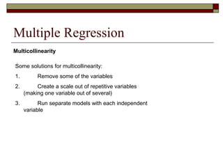
Multiple Regression
Some solutions for multicollinearity:
1. Remove some of the variables
2. Create a scale out of repetitive variables
(making one variable out of several)
3. Run separate models with each independent
variable
Multicollinearity

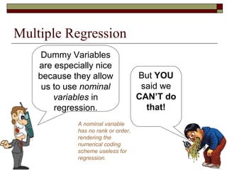
Multiple Regression
 Dummy Variables
 They are simply dichotomous variables that are entered into
regression. They have 0 – 1 coding where 0 = absence of
something and 1 = presence of something. E.g., Female
(0=M; 1=F) or Southern (0=Non-Southern; 1=Southern).
What are
dummy
variables?!

Multiple Regression
But YOU
said we
CAN’T do
that!
A nominal variable
has no rank or order,
rendering the
numerical coding
scheme useless for
regression.
Dummy Variables
are especially nice
because they allow
us to use nominal
variables in
regression.

Multiple Regression
 The way you use nominal variables in regression is by
converting them to a series of dummy variables.
Recode into different
Nomimal Variable Dummy Variables
Race 1. White
1 = White 0 = Not White; 1 = White
2 = Black 2. Black
3 = Other 0 = Not Black; 1 = Black
3. Other
0 = Not Other; 1 = Other

Multiple Regression
 The way you use nominal variables in regression is by converting them to
a series of dummy variables.
Recode into different
Nomimal Variable Dummy Variables
Religion 1. Catholic
1 = Catholic 0 = Not Catholic; 1 = Catholic
2 = Protestant 2. Protestant
3 = Jewish 0 = Not Prot.; 1 = Protestant
4 = Muslim 3. Jewish
5 = Other Religions 0 = Not Jewish; 1 = Jewish
4. Muslim
0 = Not Muslim; 1 = Muslim
5. Other Religions
0 = Not Other; 1 = Other Relig.

Multiple Regression
 When you need to use a nominal variable in
regression (like race), just convert it to a
series of dummy variables.
 When you enter the variables into your
model, you MUST LEAVE OUT ONE OF
THE DUMMIES.
Leave Out One Enter Rest into Regression
White Black
Other

Multiple Regression
 The reason you MUST LEAVE OUT ONE OF THE
DUMMIES is that regression is mathematically
impossible without an excluded group.
 If all were in, holding one of them constant would
prohibit variation in all the rest.
Leave Out One Enter Rest into Regression
Catholic Protestant
Jewish
Muslim
Other Religion

Multiple Regression
 The regression equations for dummies will
look the same.
For Race, with 3 dummies, predicting self-esteem:
Y = a + b1X1 + b2X2
∧
a = the y-intercept,
which in this case is
the predicted value
of self-esteem for
the excluded group,
white.
b1 = the slope
for variable
X1, black
b2 = the slope
for variable
X2, other

Multiple Regression
 If our equation were:
For Race, with 3 dummies, predicting self-esteem:
Y = 28 + 5X1 – 2X2
a = the y-intercept,
which in this case is
the predicted value
of self-esteem for
the excluded group,
white.
5 = the slope
for variable
X1, black
-2 = the slope
for variable
X2, other
∧
Plugging in values for
the dummies tells you
each group’s self-esteem
average:
White = 28
Black = 33
Other = 26
When cases’ values for X1 = 0 and X2 = 0, they are white;
when X1 = 1 and X2 = 0, they are black;
when X1 = 0 and X2 = 1, they are other.

Multiple Regression
 Dummy variables can be entered into multiple
regression along with other dichotomous and
continuous variables.
 For example, you could regress self-esteem
on sex, race, and education:
Y = a + b1X1 + b2X2 + b3X3 + b4X4
How would you interpret this?
Y = 30 – 4X1 + 5X2 – 2X3 + 0.3X4
X1 = Female
X2 = Black
X3 = Other
X4 = Education
∧
∧

Multiple Regression
Y = 30 – 4X1 + 5X2 – 2X3 + 0.3X4
 Women’s self-esteem is 4 points lower than men’s.
 Blacks’ self-esteem is 5 points higher than whites’.
 Others’ self-esteem is 2 points lower than whites’
and consequently 7 points lower than blacks’.
 Each year of education improves self-esteem by 0.3
units.
X1 = Female
X2 = Black
X3 = Other
X4 = Education
∧

Multiple Regression
Y = 30 – 4X1 + 5X2 – 2X3 + 0.3X4
Plugging in some select values, we’d get self-esteem for
select groups:
 White males with 10 years of education = 33
 Black males with 10 years of education = 38
 Other females with 10 years of education = 27
 Other females with 16 years of education = 28.8
X1 = Female
X2 = Black
X3 = Other
X4 = Education
∧

Multiple Regression
Y = 30 – 4X1 + 5X2 – 2X3 + 0.3X4
The same regression rules apply. The slopes represent
the linear relationship of each independent variable
in relation to the dependent while holding all other
variables constant.
X1 = Female
X2 = Black
X3 = Other
X4 = Education
∧
Make sure you get into the habit of saying
the slope is the effect of an independent
variable “while holding everything else
constant.”

Multiple Regression
Y = 30 – 4X1 + 5X2 – 2X3 + 0.3X4
The same regression rules apply…
R2
tells you the proportion of variation in your dependent
variable that explained by your independent variables
The significance tests tell you whether your null hypotheses
are to be rejected or not. If they are rejected, you have a low
probability that your sample could have come from a
X1 = Female
X2 = Black
X3 = Other
X4 = Education
∧

Multiple Regression
Interactions
Another very important concept in multiple regression is
“interaction,” where two variables have a joint effect on the
dependent variable. The relationship between X1 and Y is affected
by the value each person has on X2.
For example:
Wages (Y) are decreased by being black (X1), and wages (Y) are
decreased by being female (X2). However, being a black woman
(X1* X2) increases wages relative to being a black man.

Multiple Regression
 One models for interactions by creating a new
variable that is the cross product of the two variables
that may be interacting, and placing this variable into
the equation with the original two.
 Without interaction, male and female slopes create
parallel lines, as do black and white.
 Wages = 28k - 3k*Black - 1k*Female^
28k
25k
0 1
men
women
27k
24k
Black
28k
27k
0 1
white
black
25k
24k
Female

Multiple Regression
 One models for interactions by creating a new
variable that is the cross product of the two variables
that may be interacting, and placing this variable into
the equation with the original two.
 With interaction, male and female slopes do not have
to be parallel, nor do black and white slopes.
 Wages = 28k - 3k*Black - 1k*Female + 2k*Black*Female^
28k
25k
0 1
men
women
27k
26k
Black
28k
27k
0 1
white
black25k 26k
Female

Multiple Regression
 Let’s look at another example…
 Sex and Education may affect Wages as such:
Wages = 20k - 1k*Female + .3k*Education
But there is reason to think that men get a higher
payout for education than women.
With the interaction, the equation may be:
Wages = 19k - 1k*F + .4k*Educ - .2k*F*Educ
^
^

Multiple Regression
With the interaction, the equation may be:
Wages = 19k - 1k*F + .4k*Educ - .2k*F*Educ
0 10 20 Education
30k
20kWages
men
women
The results show different slopes for the increase in
wages for women and men as education increases.

Multiple Regression
 When one suspects that interactions may be
occurring in the social world, it is appropriate to test
for them.
 To test for an interaction, enter an “interaction term”
into the regression along with the original two
variables.
 If the interaction slope is significant, you have
interaction in the population. Report that!
 If the slope is not significant, remove the interaction
term from your model.

Multiple Regression
Standardized Coefficients
 Sometimes you want to know whether one variable
has a larger impact on your dependent variable than
another.
 If your variables have different units of measure, it is
hard to compare their effects.
 For example, if wages go up one thousand dollars
for each year of education, is that a greater effect
than if wages go up five hundred dollars for each
year increase in age.

Multiple Regression
 So which is better for increasing wages, education or
aging?
 One thing you can do is “standardize” your slopes so
that you can compare the standard deviation increase
in your dependent variable for each standard
deviation increase in your independent variables.
 You might find that Wages go up 0.3 standard
deviations for each standard deviation increase in
education, but 0.4 standard deviations for each
standard deviation increase in age.

Multiple Regression
 Recall that standardizing regression coefficients is
accomplished by the formula: b(Sx/Sy)
 In the example above, education and income have very
comparable effects on number of children.
 Each lowers the number of children by .4 standard deviations
for a standard deviation increase in each, controlling for the
other.
Coefficientsa
11.770 1.734 6.787 .000
-.364 .173 -.412 -2.105 .047
-.403 .194 -.408 -2.084 .049
(Constant)
Education
Income
Model
1
B Std. Error
Unstandardized
Coefficients
Beta
Standardized
Coefficients
t Sig.

Multiple Regression
 One last note of caution...
 It does not make sense to standardize slopes for
dichotomous variables.
 It makes no sense to refer to standard deviation increases
in sex, or in race--these are either 0 or they are 1 only.

Multiple Regression
Nested Models
 “Nested models” refers to starting with a smaller set of
independent variables and adding sets of variables in stages.
 Keeping the models smaller achieves parsimony, simplest
explanation.
 Sometimes it makes sense to see whether adding a new set of
variables improves your model’s explanatory power
(increases R2
).
 For example, you know that sex, race, education and age
affect wages. Would adding self-esteem and self-efficacy
help explain wages even better?

Multiple Regression
Nested Models
Y = a + b1X1 + b2X2 + b3X3 ReducedModel
Y = a + b1X1 + b2X2 + b3X3 + b4X4 + b5X5 CompleteModel
 You should start by seeing whether the coefficients are
significant.
 Another test, to see if they jointly improve your model, is the
change in R2
test (which you can request from SPSS)
R2
c - R2
r/df=#extra slopes in complete
F =
1 - R2
c / df=#slopes+1 in complete
Nested
Models

Multiple Regression
Nested Models with Change in R2
Dependent Variable: How often does S attend religious
services. Higher values equal more often.
Model 1 Model 2
Female Female
White (W=1) White
Black (B=1) Black
Age Age
Education

Multiple Regression
Dependent Variable: How often does S attend religious services. Higher values equal more
often. Model Summary
.232a .054 .052 2.632 .054 38.565 4 2724 .000
.249b .062 .060 2.622 .008 23.763 1 2723 .000
Model
1
2
R R Square
Adjusted
R Square
Std. Error of
the Estimate
R Square
Change F Change df1 df2 Sig. F Change
Change Statistics
Predictors: (Constant), AGE OF RESPONDENT, female = 1, Black, Whitea.
Predictors: (Constant), AGE OF RESPONDENT, female = 1, Black, White, HIGHEST YEAR OF SCHOOL COMPLETEDb.
ANOVAc
1068.987 4 267.247 38.565 .000a
18876.482 2724 6.930
19945.469 2728
1232.295 5 246.459 35.863 .000b
18713.174 2723 6.872
19945.469 2728
Regression
Residual
Total
Regression
Residual
Total
Model
1
2
Sum of
Predictors: (Constant), AGE OF RESPONDENT, female = 1, Black, Whitea.
Predictors: (Constant), AGE OF RESPONDENT, female = 1, Black, White, HIGHEST
YEAR OF SCHOOL COMPLETED
b.
Dependent Variable: HOW OFTEN R ATTENDS RELIGIOUS SERVICESc.

Multiple Regression
Dependent Variable: How often does S attend religious services. Higher values equal more often.
Coefficientsa
2.298 .232 9.887 .000
.783 .102 .144 7.698 .000
-.116 .205 -.017 -.566 .572
.894 .237 .116 3.779 .000
.019 .003 .124 6.561 .000
1.110 .336 3.302 .001
.777 .101 .143 7.674 .000
-.140 .204 -.021 -.688 .492
.966 .236 .125 4.093 .000
.021 .003 .135 7.157 .000
.084 .017 .092 4.875 .000
(Constant)
female = 1
White
Black
AGE OF RESPONDENT
(Constant)
female = 1
White
Black
AGE OF RESPONDENT
HIGHEST YEAR OF
SCHOOL COMPLETED
Model
1
2
B Std. Error
Unstandardized
Coefficients
Beta
Standardized
Coefficients
t Sig.
Dependent Variable: HOW OFTEN R ATTENDS RELIGIOUS SERVICESa.

Multiple Regression
 Females attend services more often than males.
 Blacks attend services more often than whites and
others.
 Older persons attend services more often than
younger persons.
 The more educated a person is, the more often he or
she attends religious services.
 Education adds to the explanatory power of the
model.
 Only five to six percent of the variation in religious
service attendance is explained by our models.

multiple regression

Recommended

More Related Content

What's hot (20)

Similar to multiple regression (20)

Recently uploaded (20)

multiple regression