 for null value
✌
✆](https://image.slidesharecdn.com/notesonoctave-cloneofmatlab-02of02byarunumrao-211010171923/85/Notes-for-GNU-Octave-Numerical-Programming-for-Students-02-of-02-by-arun-umrao-1-320.jpg)

✌
✆
2.2.1 Is Variable Global
isglobal is used to find whether a variable is global or not. It returns ‘true’ if
variable is global otherwise ‘false’.
✞
>>> global x; # global variable x
2 >>> isglobal ("x")
✌
✆
✞
ans = 1
✌
✆
2.3 Persistant Of a Variable
A variable that has been declared persistent within a function will retain its con-
tents in memory between subsequent calls to the same function. The difference
between persistent variables and global variables is that persistent variables are
local in scope to a particular function and are not visible elsewhere.
✞
1 >>> global x=1; # global scope; can be called or copy
anywhere
>>> isglobal ("x")
3 >>> function f(y);
>>> y=2; #local scope; within the function body
5 >>> endfunction
✌
✆
✞
ans = 1
✌
✆
2.3.1 Clear Symbol From Table (clear)
Delete the names matching the given patterns from the symbol table. The
pattern may contain the following special characters:
1. ‘?’ : Match any single character.
2. ‘*’ : Match zero or more characters.
3. ‘[ ¡list¿ ]’ : Match the list of characters specified by list.
If the first character is ‘!’ or ‘ˆ’ then matching of all characters is performed
excepting those specified by a list. For example, the pattern [a-zA-Z]’ will match
all lower and upper case alphabetic characters. For example](https://image.slidesharecdn.com/notesonoctave-cloneofmatlab-02of02byarunumrao-211010171923/85/Notes-for-GNU-Octave-Numerical-Programming-for-Students-02-of-02-by-arun-umrao-2-320.jpg)


![158 Functions
Now, here are two forms of outputs. If called a function with terminating
symbol, then only user defined out variable is shown in the screen. Similarly,
when called function is not terminated, then both user defined output variable
and default output variable are shown in the screen. Her, the function can be
called in its standard form too:
✞
>>> [a]= myAvg (4,5);
✌
✆
✞
o = 4.5000
✌
✆
✞
1 >>> [a]= myAvg (4,5)
✌
✆
✞
o = 4.5000
a = 4.5000
✌
✆
Arguments and their corresponding values may also be assigned in ‘argument
list’ region.
✞
>>> function myFunc(msg="Hello!!!")
2 >>> printf(msg);
>>> endfunction
4 >>> myFunc ()
✌
✆
✞
Hello !!!
✌
✆
The multiple output variables can be used in a function if output variables are
arranged in a vector form. Each element has unique output value and they are
independent of each other.
✞
1 >>> function [<ret vector >] = <func name >(<args list >)
>>> <contents of function i.e. body >
3 >>> endfunction
✌
✆
Example is
✞
1 >>> x=0;
>>> function [y, z]= myFunc(x)
3 >>> y = x/10;
>>> z = x*2;
5 >>> endfunction
>>> [y,z]= myFunc (10)
✌
✆
✞
y = 1
z = 20
✌
✆](https://image.slidesharecdn.com/notesonoctave-cloneofmatlab-02of02byarunumrao-211010171923/85/Notes-for-GNU-Octave-Numerical-Programming-for-Students-02-of-02-by-arun-umrao-8-320.jpg)
![3.1. FUNCTION 159
https://sites.google.com/view/arunumrao
If output variables are more than the return values in the function statements
then output variables without return value in the statement of the body are
assigned as null value.
✞
>>> x=0;
2 >>> function [y, z, t]= myFunc(x)
>>> y = x/10;
4 >>> z = x*2;
>>> # t is not assigned any return value
6 >>> endfunction
>>> [y,z,t]= myFunc (10)
✌
✆
✞
y = 1
z = 20
t = [](0 x0)
✌
✆
3.1.2 Arguments
Arguments are those values which are passed to a function. These arguments
are used by the function itself for its internal operations.
✞
1 >>> Func (<argument 1>, <argument 2>, ..., <argument n>)
✌
✆
3.1.3 Key Words
Some function names are used by Software itself. These function names can not
be redefined or reused by the program. Followings are the key words used by
Octave itself.
case catch classdef continue
do else elseif end
end try catch end unwind protect endclassdef endenumeration
endevents endfor endfunction endif
endmethods endparfor endproperties endswitch
endwhile enumeration events for
function global if methods
otherwise parfor persistent properties
return static switch try
until unwind protect unwind protect cleanup while](https://image.slidesharecdn.com/notesonoctave-cloneofmatlab-02of02byarunumrao-211010171923/85/Notes-for-GNU-Octave-Numerical-Programming-for-Students-02-of-02-by-arun-umrao-9-320.jpg)

![3.1. FUNCTION 161
https://sites.google.com/view/arunumrao
✞
>>> format long ;
2 >>> pi
✌
✆
✞
ans =
3.14159265358979
✌
✆
✞
>>> format hex;
2 >>> pi
✌
✆
✞
ans =
400921fb 54442d18
✌
✆
3.1.7 Number of Input Arguments (nargin)
Octave has a table list called nargin that stores the variables of any size. Each
time a function is called, nargin is automatically initialized to the number of
arguments that have actually been passed to the function.
✞
>>> x=0;
2 >>> function [y, z] = myFunc(x)
>>> y = x/10;
4 >>> z = nargin;
>>> endfunction
6 >>> [y, z] = myFunc (10)
✌
✆
✞
y = 1
z = 1
✌
✆
nargin also tells about the number of arguments a function can accept.
✞
>>> x=0;
2 >>> function y=myFunc(x)
>>> y = x/2;
4 >>> endfunction
>>> function z=myFuncA(x,y)
6 >>> z = (x+y)/2;
>>> endfunction
8 >>> nargin("myFunc")
>>> nargin("myFuncA ")
✌
✆
✞
ans = 1
ans = 2
✌
✆](https://image.slidesharecdn.com/notesonoctave-cloneofmatlab-02of02byarunumrao-211010171923/85/Notes-for-GNU-Octave-Numerical-Programming-for-Students-02-of-02-by-arun-umrao-11-320.jpg)
![162 Functions
3.1.8 Number of Output Arguments (nargout)
nargout tells about the number of return arguments present in the function
definition.
✞
>>> x=0;
2 >>> function y = myFunc(x)
>>> y = x/2;
4 >>> endfunction
>>> function [z, t] = myFuncA(x, y)
6 >>> z = (x+y)/2;
>>> endfunction
8 >>> nargout ("myFunc")
>>> nargout ("myFuncA")
✌
✆
✞
ans = 1
ans = 2
✌
✆
3.1.9 How to Use a Function (usage)
If a function is not called properly, then this function tells about the proper use
of the function. See in the following example:
✞
>>> x=0;
2 >>> function [y, z]= myFunc(x)
>>> if (nargin != 1)
4 >>> usage ("myFunc (<vector >)");
>>> else
6 >>> y=x/10;
>>> z = nargin;
8 >>> endif
>>> endfunction
10 >>> [y,z]= myFunc()
✌
✆
✞
usage: myFunc (<vector >)
✌
✆
3.1.10 Error (error)
This function is used to show the error occurs if any.
✞
1 >>> x=0;
>>> function y=myFunc(x)
3 >>> if (! isvector (x))
>>> y = x/2;](https://image.slidesharecdn.com/notesonoctave-cloneofmatlab-02of02byarunumrao-211010171923/85/Notes-for-GNU-Octave-Numerical-Programming-for-Students-02-of-02-by-arun-umrao-12-320.jpg)
![3.1. FUNCTION 163
https://sites.google.com/view/arunumrao
5 >>> else
>>> error("x should not be a vector.");
7 >>> endif
>>> endfunction
9 >>> myFunc ([10 ,20 ,30])
✌
✆
✞
error: x should not be a vector.
✌
✆
3.1.11 Error Number (errno)
It returns the current value of the system-dependent variable errno.
✞
1 >>> err = errno ()
✌
✆
‘err’ will be zero if there is no error otherwise error number if there is an error.
3.1.12 List of Error Numbers (errno list)
errno list returns the list of errors and their corresponding numbers.
✞
1 >>> errno_list
✌
✆
✞
ans =
{
E2BIG = 7
EACCES = 13
EAGAIN = 11
......
EXDEV = 18
}
✌
✆
3.1.13 Last Error (lasterr)
lasterr returns the error encountered to Octave most recently during the current
session.
✞
>>> lasterr;
✌
✆
3.1.14 Last Warning (lastwarn)
lastwarn returns the recent most warning shown by the Octave during the ses-
sion. If there is not any warning during the session, it return empty result.
✞
1 >>> lastwarn ;
✌
✆](https://image.slidesharecdn.com/notesonoctave-cloneofmatlab-02of02byarunumrao-211010171923/85/Notes-for-GNU-Octave-Numerical-Programming-for-Students-02-of-02-by-arun-umrao-13-320.jpg)
![164 Functions
3.1.15 Variable Input Arguments (varargin)
varargin appears as one argument of a function and it stores the number of
arguments that can be accept by a function. varargin list is initialized auto-
matically when a function is initialized. In other words, if user wants to supply
variable numbers of arguments to a function then argument varargin should be
used as a function argument. The syntax is
✞
1 >>> function [<return value vector >] = <function name by
user >( varargin )
>>> disp (varargin {i}) #ith element of variable argument
3 >>> endfunction
✌
✆
Example is
✞
1 >>> function myVarFunc (varargin )
>>> for i=1: length(varargin )
3 >>> disp (varargin {i});
>>> disp ("n");
5 >>> endfor
>>> endfunction
7 >>> myVarFunc (10, 20, 30)
>>> myVarFunc (10, 20, 30, 40)
✌
✆
✞
ans =
10
20
30
ans =
10
20
30
40
✌
✆
3.1.16 Variable Output Arguments (varargout)
varargout returns variable outputs. varargout list is initialized automatically
when a function is initialized. The syntax is
✞
1 >>> function varargout = <function name by user >( varargin )
>>> varargout {i}=i #ith element as ith out argument
3 >>> endfunction
✌
✆
Example is](https://image.slidesharecdn.com/notesonoctave-cloneofmatlab-02of02byarunumrao-211010171923/85/Notes-for-GNU-Octave-Numerical-Programming-for-Students-02-of-02-by-arun-umrao-14-320.jpg)
![3.1. FUNCTION 165
https://sites.google.com/view/arunumrao
✞
1 >>> function varargout = myVarFunc (varargin )
>>> for i=1: length(varargin )
3 >>> varargout {i}= varargin {i};
>>> endfor
5 >>> endfunction
>>> [a, b, c, d] = myVarFunc (10, 20, 30)
✌
✆
✞
ans =
10
20
30
error: element number 4 undefined in return list
✌
✆
3.1.17 Tilde ( )
is used in place of input argument name of a function to ignore the corre-
sponding argument value and not stored it to any variable. Syntax is
✞
1 >>> function [<ret vector >] = <func name >(~, <other arg(s) >)
>>> val = <any other argument >
3 >>> endfunction
✌
✆
The working example is
✞
1 >>> x=0;
>>> function myFunc(~, x)
3 >>> y = x+2;
>>> endfunction
5 >>> myFunc(10, 20)
✌
✆
✞
ans = 22
✌
✆
The value of nargin is not affected by using this declaration.
3.1.18 Whether Argument is Out Type (isargout)
isargout returns ‘true’ if string is a valid out argument otherwise returns ‘false’.
✞
1 >>> x=0;
>>> function y = myFunc(~, x)
3 >>> isargout (1) # true as y is out argument
>>> isargout (2) # false as there is no
5 >>> # second out argument
>>> y=x+2;
7 >>> endfunction
>>> myFunc(10, 20)
✌
✆](https://image.slidesharecdn.com/notesonoctave-cloneofmatlab-02of02byarunumrao-211010171923/85/Notes-for-GNU-Octave-Numerical-Programming-for-Students-02-of-02-by-arun-umrao-15-320.jpg)


![172 Conditional Function
✞
1 >>> for i=1:5
>>> i
3 >>> endfor
✌
✆
✞
i = 1
i = 2
i = 3
i = 4
i = 5
✌
✆
for statement also accepts the array elements for performing loop.
✞
1 >>> for i={1,2, "A"}
>>> i
3 >>> endfor
✌
✆
✞
i =
{
[1,1] = 1
}
i =
{
[1,1] = 2
}
i =
{
[1,1] = A
}
✌
✆
Here each [1,1] represents the rows and columns of each array element. A two
dimensional array may also be used.
✞
>>> for i={1 ,2;"A","B"}
2 >>> i
>>> endfor
✌
✆
✞
i =
{
[1,1] = 1
[2,1] = A
}
i =
{
[1,1] = 2
[2,1] = B
}
✌
✆](https://image.slidesharecdn.com/notesonoctave-cloneofmatlab-02of02byarunumrao-211010171923/85/Notes-for-GNU-Octave-Numerical-Programming-for-Students-02-of-02-by-arun-umrao-22-320.jpg)
![4.1. LOOP CONDITION 173
https://sites.google.com/view/arunumrao
for statement and matrix expression may be correlated with each other. The
method is given in following example.
✞
>>> for i=[1 ,2;3 ,4]
2 >>> i
>>> endfor
✌
✆
✞
i =
1
3
i =
2
4
✌
✆
In above procedure, columns are executed in one iteration. An key-value relation
of for statement is
✞
>>> x.a=1; # Set key ’a’ for value ’1’
2 >>> x.b=2; # Set key ’b’ for value ’2’
>>> ## Call value and key from variable ’x’ in matrix form
4 >>> for [val , key]=x;
>>> key # Print key
6 >>> val # Print value
>>> endfor # End for loop
✌
✆
✞
key = a
val = 1
key = b
val = 2
✌
✆
4.1.2 While Condition (while)
while statement performs looping until the condition is met.
✞
>>> i=1;
2 >>> while(i<10)
>>> i
4 >>> i++;
>>> endwhile
✌
✆
✞
i = 3
i = 4
i = 5
i = 6
i = 7](https://image.slidesharecdn.com/notesonoctave-cloneofmatlab-02of02byarunumrao-211010171923/85/Notes-for-GNU-Octave-Numerical-Programming-for-Students-02-of-02-by-arun-umrao-23-320.jpg)


![180 File Operation
5.1.4 Parent Machine (isdeployed)
isdeployed checks whether Octave is running in same machine in which it is
compile or not. If it is running in other machine, it returns ‘true’ value otherwise
‘false’ value.
✞
1 >>> isdeployed ()
✌
✆
✞
ans = 0
✌
✆
5.1.5 Version (version)
It returns the version of the Octave.
✞
1 >>> v = version ()
✌
✆
5.1.6 License (license)
It returns the license of the Octave.
✞
1 >>> v = license ()
✌
✆
✞
v = GNU General Public License
✌
✆
5.2 Directory Management
In this section we will discuss about the creation of directory, files, their access-
ing, reading, renaming, deletion etc.
5.2.1 Make a Dir (mkdir)
mkdir creates a directory in the current path used by Octave. If directory is
present then it just returns true value. If a directory is successfully created, it
returns true value otherwise false value. Syntax is
✞
1 >>> [STATUS , MSG , MSGID] = mkdir (PARENT , DIR)
✌
✆
Example of creating a directory “a” is
✞
1 >>> mkdir("a");
✌
✆
The output is](https://image.slidesharecdn.com/notesonoctave-cloneofmatlab-02of02byarunumrao-211010171923/85/Notes-for-GNU-Octave-Numerical-Programming-for-Students-02-of-02-by-arun-umrao-30-320.jpg)

![182 File Operation
5.2.7 Read Directory (readdir)
readdir reads the directory whose name is supplied as argument to the function.
Syntax is given below
✞
1 >>> [files , error , msg] = readdir (< directory name >)
✌
✆
It returns three output handlers. First array is the list of all files inside the
directory. Second array is error type encounters while Octave tries to read
the directory and third is message returned by Octave when it read directory
successfully or not.
5.2.8 Temporary Directory (tempdir)
It returns the path of temporary directory used by the Octave for temporary
operation/execution. In this directory, temporary files are used for internal ap-
plication of Octave. When the session or application of Octave ended, temporary
files are removed from the directory. This function is used like
✞
1 >>> tempdir
✌
✆
Another method is
✞
1 >>> tempdir ()
✌
✆
✞
ans = C: DOCUME ~1 ADMINI ~1 LOCALS ~1 Temp
✌
✆
5.2.9 Temporary Name (tempname)
It returns the name of temporary directory used by the Octave for temporary
operation/execution. User can set another directory as temporary directory as
and when required. Use this function
✞
1 >>> tempname
✌
✆
✞
1 >>> tempname ()
✌
✆
✞
ans = C: DOCUME ~1 ADMINI ~1 LOCALS ~1 Temp oct -2
✌
✆](https://image.slidesharecdn.com/notesonoctave-cloneofmatlab-02of02byarunumrao-211010171923/85/Notes-for-GNU-Octave-Numerical-Programming-for-Students-02-of-02-by-arun-umrao-32-320.jpg)
![5.2. DIRECTORY MANAGEMENT 183
https://sites.google.com/view/arunumrao
5.2.10 Attribute of File (fileattrib)
It returns the attributes of a file supplied as argument to the function. The
syntax of this function is
✞
1 >>> [status , result , msgid] = fileattrib (<file path >)
✌
✆
If Octave is successful in getting of attribute ‘status’ is ‘1’. ‘result’ returns arrays
of the result on successful retrieval of attributes. ‘msgid’ is id of message shown
by Octave if any.
5.2.11 File Marker (filemarker)
It is used to find or set the character used to separate file-name from the the
sub-function names contained within the file. The syntax is
✞
1 >>> val = filemarker () # for query
>>> filemarker (<new val >, " local") # for set the character
✌
✆
5.2.12 File Parts (fileparts)
fileparts returns the directory in which file is placed, name of file, extension of
file and version. Syntax is
✞
>>> [dir , name , ext , ver] = fileparts (<file name >)
✌
✆
5.2.13 File Separator (filesep)
filesep returns the separator of directory/file in path name. It may be forward
slash or backward slash. File separator depends on the Operating System used
by Octave.
✞
1 >>> filesep
✌
✆
✞
ans =
✌
✆
5.2.14 Copy File (copyfile)
copyfile copies a file with another name. The path of directory may be relative
or absolute. Syntax is
✞
1 >>> [status , msg , msgid] =
>>> copyfile (<source file >, <dest file >)
✌
✆](https://image.slidesharecdn.com/notesonoctave-cloneofmatlab-02of02byarunumrao-211010171923/85/Notes-for-GNU-Octave-Numerical-Programming-for-Students-02-of-02-by-arun-umrao-33-320.jpg)
![184 File Operation
If the destination file exists, it overwrites the destination file by the file being
copied without any warning.
5.2.15 Move File (movefile)
movefile moves a file from one directory to another directory. The path of
directory may be relative or absolute. Syntax is
✞
>>> [status , msg , msgid] =
2 >>> movefile (<source file >, <dest file >)
✌
✆
‘status’ handle returns the status of the operation, ‘msg’ returns message and
‘msgid’ is the id of the last message shown by Octave.
5.2.16 Rename a File (rename)
rename renames a file name with another file name. Syntax is
✞
>>> [err , msg] = rename (<old name >, <new name >)
✌
✆
It shows error if there is any error arises during this process & message if any
returned by the Octave.
5.2.17 Delete a File (unlink)
unlink deletes a file. Syntax is
✞
1 >>> [err , msg] = unlink(<file name >)
✌
✆
It shows error if there is any error arises during this process & message if any
returned by the Octave.
5.3 I/O Operation
Reading, writing and managing of a file is known as file operation. Input and
output operations are reading and writing of a file. The functions which are
used in file reading and writing are explained below.
5.3.1 End of File (feof)
Returns ‘1’ if an end-of-file condition has been encountered for a given file
and ‘0’ otherwise. It will only return ‘1’ if the end of the file has already been
encountered otherwise next read operation will result in an end-of-file condition.](https://image.slidesharecdn.com/notesonoctave-cloneofmatlab-02of02byarunumrao-211010171923/85/Notes-for-GNU-Octave-Numerical-Programming-for-Students-02-of-02-by-arun-umrao-34-320.jpg)


![5.3. I/O OPERATION 187
https://sites.google.com/view/arunumrao
5.3.10 Scan a Value (scanf)
scanf scans input stream according to the template string. The syntax is
✞
1 >>> [val , count] = scanf (<template >, <size >)
✌
✆
It returns the scanned value and number of bytes scanned in vector form.
5.3.11 Formatted Scanning (sscanf)
sscanf reads string in format based on template and copies it into output stream.
The syntax is
✞
1 >>> [val , count , errmsg , pos] =
>>> sscanf (<input >, <template >, <variable >)
✌
✆
It returns ‘true’ value if fscanf reads data successfully.
5.3.12 Rewind a Pointer (frewind)
frewind sets the file pointer to the beginning of the file, returning 0 for success,
and ‘-1’ if an error is encountered.
✞
>>> f=fopen(" myfile.txt","r");
2 >>> ipos = ftell(f) # Show the current position
>>> fgets(f,4); # Read the file four bytes
4 >>> ## Set the current position to four bytes from
>>> ## from begining of file .
6 >>> fseek(f,4, SEEK_SET );
>>> cpos = ftell(f) # Get the current file pointer.
8 >>> frewind(f) # Set pointer at the beginning of file .
>>> fpos = ftell(f) # Get the current position of file
pointer.
10 >>> fclose(f); # Close the file .
✌
✆
The output is
✞
ipos = = 0
cpos = = 4
fpos = = 0
✌
✆
5.3.13 Scan to Buffer (fscanf)
fscanf reads data from file stream and copies it into buffer stream. The syntax
is](https://image.slidesharecdn.com/notesonoctave-cloneofmatlab-02of02byarunumrao-211010171923/85/Notes-for-GNU-Octave-Numerical-Programming-for-Students-02-of-02-by-arun-umrao-37-320.jpg)
![188 File Operation
✞
1 >>> [val , count , errmsg] =
>>> fscanf (<in file id >, <template >, <variable >)
✌
✆
It returns ‘true’ value if fscanf reads data successfully.
5.3.14 Get Pointer Position (fseek)
A pointer is positioned at offset pointer from the beginning of a file during the
read mode of the file. Offset may be one of the predefined variables SEEK CUR
(current position), SEEK SET (beginning), or SEEK END (end of file) or strings
“cof”, “bof” or “eof”. If origin is omitted, SEEK SET is assumed by default.
Offset may be positive, negative, or zero but not all combinations of origin and
offset can be realized.
✞
>>> f=fopen("myfile.txt","r");
2 >>> ipos = ftell(f) # Show the current position
>>> fgets(f,4); # Read the file four bytes
4 >>> ## Set the current position after
>>> ## four bytes from begining of a file .
6 >>> fseek(f, 4, SEEK_SET );
>>> fpos = ftell(f) # Get the current position of file .
8 >>> fclose(f); # Close the file .
✌
✆
The output is
✞
ipos = 0
fpos = 4
✌
✆
5.3.15 Pointer Position (ftell)
ftell returns the current position of file pointer from the beginning of file. The
position of file pointer is updated when a file is either read or wrote. fseek also
updates the current position of file pointer.
✞
>>> f=fopen("myfile.txt","r");
2 >>> ftell(f)
>>> fclose(f);
✌
✆
The output is
✞
ans = 0
✌
✆
5.4 Reading Files
Here we will discuss the function those are used in reading files.](https://image.slidesharecdn.com/notesonoctave-cloneofmatlab-02of02byarunumrao-211010171923/85/Notes-for-GNU-Octave-Numerical-Programming-for-Students-02-of-02-by-arun-umrao-38-320.jpg)

![190 File Operation
✞
1 >>> f = fopen ("myfile.txt","r");
>>> dt = fskipl (f) # skips only one line
3 >>> fclose (f);
✌
✆
If number of line is ‘Inf’ then all the lines will be skipped until EOF is not
encountered.
✞
1 >>> f = fopen ("myfile.txt","r");
>>> dt = fskipl (f,Inf) # skips infinite lines
3 >>> fclose (f);
✌
✆
5.4.4 Read File in Binary (fread)
fread is used to read a file in binary format. The syntax of this function is
✞
1 >>> count = fread(
>>> <file_id >,
3 >>> <buffer_size >,
>>> <precision >,
5 >>> <skip >,
>>> <architecture >
7 >>> )
✌
✆
Here, ‘file id’ is id of previously opened file. Argument ‘buffer size’ tells that
how many binary data is to be read from stream file. The optional ‘buffer size’
values are given in the following table.
Buffer Size Description
Integer It is for specific number of data bytes.
Inf Read data as much as possible.
[r, Inf] Read data as much as possible, return-
ing a matrix with ‘r’ rows. If the
number of elements read is not an ex-
act multiple of ‘r’, the last column is
padded with zeros.
[r, c] Read data by r × c elements, returning
a matrix with ‘r’ rows. If the number of
elements read is not an exact multiple
of ‘r’, the last column is padded with
zeros.](https://image.slidesharecdn.com/notesonoctave-cloneofmatlab-02of02byarunumrao-211010171923/85/Notes-for-GNU-Octave-Numerical-Programming-for-Students-02-of-02-by-arun-umrao-40-320.jpg)


![5.5. WRITING FILES 197
https://sites.google.com/view/arunumrao
✞
1 >>> f = fopen ("myfile.txt","w");
>>> dt = fwrite (f,"This is my file .","char " ,1,"ieee -be")
3 >>> fclose (f);
✌
✆
✞
T h i s i s m y f i l e .
✌
✆
5.5.3 CSV Write (csvwrite)
CSV stands for Comma Separated Value. csv write data into comma separated
value file. Each data row is terminated by semi-colon ‘;’. Data in each row
separated by space. Data should be in matrix form. Its syntax is
✞
1 >>> csvwrite (<file name >, <data handle >);
✌
✆
✞
1 >>> m = [3 6 9 12 15; 5 10 15 20 25;
>>> 7 14 21 28 35; 11 22 33 44 55];
3 >>> csvwrite (’csv1 .txt’,m)
✌
✆
With column offsets the same function is used as
✞
1 >>> csvwrite (<file name >,
>>> <data handle >,
3 >>> <number of offset rows >,
>>> <number of offset cols >
5 >>> );
✌
✆
✞
1 >>> m = [3 6 9 12 15; 5 10 15 20 25;
>>> 7 14 21 28 35; 11 22 33 44 55];
3 >>> csvwrite (’csv2 .txt’,m,1,2)
✌
✆
To formatted write, CSV files are written with dlmwrite() function.
✞
1 >>> dlmwrite (
>>> <file name >,
3 >>> <data >,
>>> <row offset >,
5 >>> <col offset >,
>>> <key name >,
7 >>> <key value >,
>>> <options >
9 >>> )
✌
✆
1. append : It is used to select append mode on or off.](https://image.slidesharecdn.com/notesonoctave-cloneofmatlab-02of02byarunumrao-211010171923/85/Notes-for-GNU-Octave-Numerical-Programming-for-Students-02-of-02-by-arun-umrao-47-320.jpg)
![198 File Operation
2. delimiter : This key is used to controll the delimiter type. A delimiter
may be any alpha-numeric character or special symbol.
3. newline : The character(s) to use to separate each row. Three special
cases exist for this option. “unix” is changed into “n”, “pc” is changed
into “rn”, and “mac” is changed into “r”. Any other value is used
directly as the newline separator.
4. precision : It controls the significant digits.
✞
1 >>> m = [3 6 9 12 15; 5 10 15 20 25;
>>> 7 14 21 28 35; 11 22 33 44 55];
3 >>> dlmwrite ("dsv.tex", m, "delimiter ", "&", "newline ",
"n");
✌
✆
5.6 GUI Building
5.6.1 Getting Directory
The directory listing or choosing dialog is opened by uigetdir() function. Syn-
opsis of this function is used one of the listed below.
✞
1 >>> dirname = uigetdir ()
>>> dirname = uigetdir (<initial path >)
3 >>> dirname = uigetdir (<initial path >, <dialog name >)
✌
✆
In example below, a dialog is opened indicating to initial path to ‘/’. After
selection of a directory and choosing it, the function returns directory name to
function handler ‘dirname’. The directory name is displayed in output by disp()
function.
✞
1 >>> dirname = uigetdir ("/","Select Directory ");
>>> disp ( dirname);
✌
✆
✞
/mnt
✌
✆
5.6.2 Getting a File
A filtered file selection can be performed by uigetfile() function by using full
discription as shown below.
✞
1 >>> [filename , filepath , fileindex ] =
>>> uigetfile (
3 >>> <filtered extension >,](https://image.slidesharecdn.com/notesonoctave-cloneofmatlab-02of02byarunumrao-211010171923/85/Notes-for-GNU-Octave-Numerical-Programming-for-Students-02-of-02-by-arun-umrao-48-320.jpg)
![5.6. GUI BUILDING 199
https://sites.google.com/view/arunumrao
>>> <dialog name >,
5 >>> <default file >,
>>> "Position ",
7 >>> [px py],
>>> "MultiSelect ",
9 >>> <mode >
>>> )
✌
✆
We can omit one or all of the inputs but “position” & [px py] and “MultiSelect”
& mode shall be omitted in pair. Selected file name is returned to ‘filename’,
file path is returned to ‘filepath’. Each file in multimode selection is assigned a
unique id to ‘fileindex’.
✞
>>> [filename , filepath , fileindex ] = uigetfile ()
✌
✆
✞
filename = b.m
filepath = /home /arun /
fileindex = 1
✌
✆
5.6.3 Process Status
Durint the process, process progress can be visualized by wait bar. Wait bar in
Octave is activated by waitbar() function. Its synopsis is
✞
1 >>> <hid >= waitbar (
>>> <fract [0, 1]>,
3 >>> <message >,
>>> <figure property 1>,
5 >>> <property 1 value >,
>>> <figure property 2>,
7 >>> <property 2 value >,
>>> .................
9 >>> .................
>>> )
✌
✆
In this function, fraction value may be in range of [0, 1]. ‘message’ is the
description about the wait bar. Properties and their corresponding values are
used simultaneously.
✞
>>> <handle id >= waitbar (0.4,"% completed ");
✌
✆
Above method is used to open a waiting bar GUI and creation of its handle
id. To update a waiting bar with new fraction value, waitbar() function is used
again as given in following syntax.
✞
1 >>> waitbar(<fraction >, <handle id >, <message >);
✌
✆](https://image.slidesharecdn.com/notesonoctave-cloneofmatlab-02of02byarunumrao-211010171923/85/Notes-for-GNU-Octave-Numerical-Programming-for-Students-02-of-02-by-arun-umrao-49-320.jpg)
![200 File Operation
New fraction value shall be updated to the waiting bar identified by ‘handle id’.
✞
1 >>> h=waitbar (0,"% completed ");
>>> for(x =0:0.01:1)
3 >>> waitbar (x,h,"% completed ");
>>> endfor
✌
✆
5.6.4 Creating a Panel
uipanel() creates a panel for arranging of controls. Its syntax is
✞
>>> <hid > = uipanel (
2 >>> "parent",
>>> <parent figure handler >,
4 >>> <property 1>,
>>> <value for property 1>,
6 >>> ..............
>>> )
✌
✆
If ‘parent’ (value “parent”) is omitted then a uipanel for the current figure is
created. If no figure is available, a new figure is created first.
✞
1 >>> f = figure;
>>> p = uipanel (
3 >>> "title", #property title
>>> "Graphics Panel", #value for property title
5 >>> "position ", #property position
>>> [.25 .25 .5 .5] #value for property position
7 >>> );
>>> b1 = uicontrol (
9 >>> "parent", #parent window
>>> p, #figure handle
11 >>> "string", #control property string
>>> "A Button", #string value
13 >>> "position ", #position property
>>> [10 10 150 40] #position value
15 >>> );
>>> e1 = uicontrol (
17 >>> "parent", #parent window
>>> p, #figure handle
19 >>> "style", #control style
>>> "edit ", #control type edit
21 >>> "string", #control property string
>>> "An edit box", #string value
23 >>> "position ", #position property
>>> [10 50 150 40] #position value
25 >>> );
>>> c1 = uicontrol (](https://image.slidesharecdn.com/notesonoctave-cloneofmatlab-02of02byarunumrao-211010171923/85/Notes-for-GNU-Octave-Numerical-Programming-for-Students-02-of-02-by-arun-umrao-50-320.jpg)
![5.6. GUI BUILDING 201
https://sites.google.com/view/arunumrao
27 >>> "parent", #parent window
>>> p, #figure handle
29 >>> "style", #control style
>>> "checkbox ", #control type edit
31 >>> "string", #control property string
>>> "A check box", #string value
33 >>> "position ", #position property
>>> [10 100 150 40] #position value
35 >>> );
✌
✆
5.6.5 User Interactive Menu
The function uimenu is used to create user interactive menus. Its syntax is like
✞
1 >>> u = uimenu(h, <property >, <value >, ....)
✌
✆
If ‘h’ is omitted then a top-level menu for the current figure is created. If ‘h’ is
given then a submenu relative to ‘h’ is created. A top level menu should have
atleast one sub menu. The properties used with this function are “accelerator”
whose value is a string that is used as shortcut key with CTRL key. “callback”
property tells about the named function that will be executed if the correspond-
ing menu is interacted. The callback function may be either string name or an
object name, i.e. function name prefixed with‘@’ symbol without double quotes.
The callback function may be a cell array with function object name and its
arguments like {@f, arg1, arg2}. “foregroundcolor” for text colours. “label”
for menu label. The label value may have a ‘&’ symbol that can be marked
as accelerator. “position” for relative menu position.The entry with the lowest
value is at the first position starting from left or top. “separator” key has ”on”
or ”off” value. If enabled it draws a separator line above the current position.
It is ignored for top level entries.
✞
1 >>> f = figure;
>>> ## create top level menu in the context menu
3 >>> m1 = uimenu (f,"label","Add");
>>> ## Create sub menu under Add top level menu
5 >>> uimenu (m1 ,"label","Display
Add","callback ","disp (’Add ’)");
>>> ## create top level menu in the context menu
7 >>> m2 = uimenu (f,"label","Save ");
>>> ## Create sub menu under Add top level menu
9 >>> uimenu (m2 ,"label","Display
Save ","callback ","disp (’Save ’)");
✌
✆](https://image.slidesharecdn.com/notesonoctave-cloneofmatlab-02of02byarunumrao-211010171923/85/Notes-for-GNU-Octave-Numerical-Programming-for-Students-02-of-02-by-arun-umrao-51-320.jpg)

![5.6. GUI BUILDING 203
https://sites.google.com/view/arunumrao
In Octave, we can listen mouse click and its location over figure by using ginput
function. It is used over graphics. We can use text function to put arbitrary
string at given location over plots. This function is used as shown below:
✞
1 >>> [x, y, btn] = ginput(<figure id >)
✌
✆
Here, x, y are coordinate values and btn is button pressed. btn value is 1 for left
click, 2 for middle mouse button press, 3 for right click and ascii code of any
other button pressed. It applications are given below:
✞
1 >>> f = figure;
>>> function AddText(h, e, t)
3 >>> txt = inputdlg ("Enter string");
>>> [x,y,b]= ginput(t);
5 >>> text (x, y, txt);
>>> endfunction
7 >>> c = uicontextmenu (f);
>>> ## create menus in the context menu
9 >>> m1=uimenu("parent",c,
>>> "label","Add Text ",
11 >>> "callback " ,{@AddText ,f});
>>> set (f, " uicontextmenu ", c);
✌
✆
5.6.8 Create Control
uicontrol() creates a control object and object id is returned as handler to it. It
is used to created simple interactive controls such as push button, check-boxes,
edit and list controls. If ‘parent’ is omitted then a uicontrol() is created for
current figure. If there is no figure then a new figure is created first. There are
following types of controls:
1. checkbox : It creates check box for on/off control.
2. edit : Creates editable text box for user input.
3. listbox : Creates a selectable list box like drop-down button.
4. popupmenu : Creates a pop up menu control which displays a list of
options for user selection.
5. pushbutton : Create a push button. Action related to push button is
performed by clicking on the button.
6. radiobutton : Create a radio button control intended to use exclusive
input in a group of radio button control.
7. slider : Creates a slider control that allows user to select an input value
by the relative position of the knob of the slider.](https://image.slidesharecdn.com/notesonoctave-cloneofmatlab-02of02byarunumrao-211010171923/85/Notes-for-GNU-Octave-Numerical-Programming-for-Students-02-of-02-by-arun-umrao-53-320.jpg)
![204 File Operation
8. text : Creates a static text control.
9. togglebutton : Creates a toggle button control that appears like a push
button. But it allows to select only one state.
These controls are invoked by style, i.e. these are values of style property.
Syntax for the function is
✞
>>> <hid > = uicontrol (
2 >>> <figure handle id >,
>>> <property 1>,
4 >>> <value for property 1>,
>>> ..............
6 >>> )
✌
✆
In the following lines of code, three user interactive controls are added into the
graphics pane.
✞
>>> f = figure;
2 >>> b1 = uicontrol (f, #figure handle
>>> "string", #control property string
4 >>> "A Button", #string value
>>> "position ", #position property
6 >>> [10 10 150 40] #position value
>>> );
8 >>> e1 = uicontrol (f, #figure handle
>>> "style", #control style
10 >>> "edit ", #control type edit
>>> "string", #control property string
12 >>> "An edit box", #string value
>>> "position ", #position property
14 >>> [10 50 150 40] #position value
>>> );
16 >>> c1 = uicontrol (f, #figure handle
>>> "style", #control style
18 >>> "checkbox ", #control type edit
>>> "string", #control property string
20 >>> "A check box", #string value
>>> "position ", #position property
22 >>> [10 100 150 40] #position value
>>> );
✌
✆
In the following figure, we have creates a slider and text control in the figure
window. The slider uses callback named function ‘cb’ to update the text control
string with the current value of slider. The controls first search callback function
in built-in function list, then in the same code script and finally the working
directory. If callback function is in same code script file, then prefer that it is
before the calling controls. In the following example, the callback function is in
the same code script.](https://image.slidesharecdn.com/notesonoctave-cloneofmatlab-02of02byarunumrao-211010171923/85/Notes-for-GNU-Octave-Numerical-Programming-for-Students-02-of-02-by-arun-umrao-54-320.jpg)
![5.6. GUI BUILDING 205
https://sites.google.com/view/arunumrao
✞
1 >>> function cb( )
>>> ## Copy the graphics data to handle g
3 >>> g = guidata (gcf);
>>> ## Get the slider value
5 >>> sv = get(g.s,’value’);
>>> ## Set the text value to slider value
7 >>> set(g.t,’string’,num2str (sv , "%10.5f"));
>>> endfunction
9 >>> ## Create a figure and handler object f
>>> f = figure(’position ’ ,[100 100 500
500],’units’,’pixels’);
11 >>> ## Retrieve the figure property structure of figure f.
>>> ## We can use gcf() function too but it returns figure
13 >>> ## data of current figure not of targeted figure
>>> h = get(f);
15 >>> ## Add a slider control . Add its handler to member s of
h
>>> h.s = uicontrol (’style’,’slider’,’position ’,
17 >>> [60 20 400 20], ’callback ’,@cb);
>>> ## The above callback function does not supplied
arguments
19 >>> ##
>>> ## Add a text control. Add its handler to member t of h
21 >>> h.t = uicontrol (’style’,’text ’,
>>> ’string ’, ’?????’,
23 >>> ’position ’ ,[60 50 400 20]) ;
>>> ## Bind the data of handler h into f
25 >>> guidata(f,h);
✌
✆
To allow the callback function with supplied arguments, the ‘callback’ key of
user interactive control object must have value in cell value structure, in which
first value is named or object callback function, and rest are arguments for the
callback function.
✞
1 >>> h.s = uicontrol (’style’,’slider’,’position ’,
>>> [60 20 400 20], ’callback ’,{@cb , 0.5});
✌
✆
But the structure of callback function being executed has two default parameters
and rest are argument parameters. The first parameter is source handle, i.e. the
user interactive control that is calling to this function, second is event, i.e. left
button click, middle button click, right button click, key press, button down or
button up etc., and rest are augment parameters. The argument parameters
may be other user interactive control handles, i.e. target control, too.
✞
>>> function cb(h, e, v)
2 >>> <function bod >
>>> endfunction
✌
✆](https://image.slidesharecdn.com/notesonoctave-cloneofmatlab-02of02byarunumrao-211010171923/85/Notes-for-GNU-Octave-Numerical-Programming-for-Students-02-of-02-by-arun-umrao-55-320.jpg)
![206 File Operation
The complete example for callback function is modified as given below:
✞
1 >>> function cb(h, e, v)
>>> g = guidata(gcf);
3 >>> sv = get(g.s,’value’);
>>> if(sv >v)
5 >>> set(g.t,’string ’,num2str(sv , "%10.5f"));
>>> endif
7 >>> endfunction
>>> f = figure(’position ’ ,[100 100 500
500],’units’,’pixels’);
9 >>> h = get(f);
>>> h.s = uicontrol (’style’,’slider’,’position ’,
11 >>> [60 20 400 20], ’callback ’,{@cb , 0.5});
>>> h.t = uicontrol (’style’,’text ’,
13 >>> ’string ’, ’?????’,
>>> ’position ’ ,[60 50 400 20]) ;
15 >>> guidata (f,h);
✌
✆
We can also pass the target object handle via uicontrol callback to the callback
function being executed. See the program given below:
✞
1 >>> function update(hs , e, ht)
>>> sv = get(hs ,’value’);
3 >>> set(ht ,’string’,num2str(sv , " %10.5f"));
>>> endfunction
5 >>> f = figure(’position ’ ,[100 100 500 500],
>>> ’units’,’pixels’);
7 >>> t1 = uicontrol (’style’,’text ’,
>>> ’string ’, ’?????’,
9 >>> ’position ’ ,[350 20 100 20]) ;
>>> s1 = uicontrol (’style’,’slider’,’position ’,
11 >>> [10 20 300 20], ’callback ’,{@update , t1});
>>> t2 = uicontrol (’style’,’text ’,
13 >>> ’string ’, ’?????’,
>>> ’position ’ ,[350 50 100 20]) ;
15 >>> s2 = uicontrol (’style’,’slider’,’position ’,
>>> [10 50 300 20], ’callback ’,{@update , t2});
✌
✆
Note that, the target handle that is being passed to callback function, must
be created before the calling of callback function as shown in above figure.
The basic callback functions that are available for all graphics objects. These
are CreateFcn that is called at the moment of the objects creation. Callbacks
that are added to CreateFcn later with the set function will never be executed.
DeleteFcn is called at the moment an object is deleted. ButtonDownFcn is
called if a mouse button is pressed while the pointer is over this object. There
are hundreds of the kye-value properties related to the user interactive controls
and toolbars. Each property can not be listed or explained here. We can get](https://image.slidesharecdn.com/notesonoctave-cloneofmatlab-02of02byarunumrao-211010171923/85/Notes-for-GNU-Octave-Numerical-Programming-for-Students-02-of-02-by-arun-umrao-56-320.jpg)

children = [](0 x1)
clipping = on
.................
units = pixels
value = 1
verticalalignment = middle
✌
✆
Be careful while applying key-value properties. A uicontrol has own specific
properties. Therefore before using a key-value property, first check it whether
it is member of the control or not by using get function as explained above.
Many properties has general meaning and purposes which are well known to
the learners, like font, font size, font weight, font type, foreground colour, back-
ground colour, color etc. For these properties the GNU-Octave help page can
be referred. Here, only important key-value properties are explained.](https://image.slidesharecdn.com/notesonoctave-cloneofmatlab-02of02byarunumrao-211010171923/85/Notes-for-GNU-Octave-Numerical-Programming-for-Students-02-of-02-by-arun-umrao-57-320.jpg)


![210 File Operation
✞
1 >>> <hui > = uitoggletool (
>>> "parent",
3 >>> <property 1>,
>>> <value for property 1>,
5 >>> .............
>>> );
✌
✆
If “parent” is omitted then a toggle button for the current figure is created. If
no figure is available, a new figure is created first. If a figure is available, but
does not contain a toggle button, a toggle button will be created.
✞
>>> f = figure ("toolbar ", "none ");
2 >>> % create empty toolbar
>>> t = uitoolbar (f);
4 >>> % create a 19 x19x3 black square
>>> img=zeros (19 ,19 ,3);
6 >>> % add uitoggletool button to toolbar
>>> b = uitoggletool (t, "cdata", img);
✌
✆
5.6.11 Dialogue Box
Dialogues are those pop-up windows which are used for specific purposes, like
showing hints, showing errors, for users’ input etc. Followings are the different
dialogues which are implemented in Octave.
✞
1 >>> h = dialog (<property >, <value >, ...)
✌
✆
Creates a transparent dialogue window in which different controls can be put
by using uicontrol function. Error showing dialogue is created as shown below:
✞
1 >>> errordlg (<Error n instructions >, <dialogue title >);
✌
✆
The hint dialogue is shown below:
✞
1 >>> h = helpdlg (msg , title)
✌
✆
The input dialogue is define as shown below:
✞
1 >>> pr = {"W", "H"}; // field labels
>>> def = {"1", "2"}; // default values
3 >>> rc = [1 ,10; 2,20; 3 ,30];// rows and cols of the input
field
>>> dims = inputdlg (pr , "Enter Box Dimensions ", rc , def);
✌
✆
Question dialogue is used with three option buttons. The return value is button
name string.](https://image.slidesharecdn.com/notesonoctave-cloneofmatlab-02of02byarunumrao-211010171923/85/Notes-for-GNU-Octave-Numerical-Programming-for-Students-02-of-02-by-arun-umrao-60-320.jpg)
![5.6. GUI BUILDING 211
https://sites.google.com/view/arunumrao
✞
>>> btn = questdlg (msg , title , btn1 , btn2 , btn3 , default );
✌
✆
To highlight the dialogue’s default button, default value should be exactly the
button name. Message dialogue is created as shown below:
✞
1 >>> msgbox (msg , title , icon );
✌
✆
Warning dialog shows fancy warning.
✞
1 >>> warndlg ({ line 1, line 2}, title);
✌
✆
The listdlg, i.e. list dialogue shows a list of available options. On clicking over
OK button after selection of the options, it returns the index of selected option.
Index count in Octave is started from one to infinite.
✞
1 >>> myO = {"A", "B", "C"};
>>> [sel , ok] = listdlg ("ListString ", myO , options);
✌
✆
The first argument is compulsory. Options are provided in a group of key-value
options. The main options are “SelectionMode” key has “Single” or “Multiple’
option values. “ListSize” is a vector which two elements in which first is width
and second is height. Default initial values are provided with “InitialValue” key.
“Name” shows the name of dialogue. “OKString” and “CancelString” are used
for naming OK button and Cancel button respectively. “PromptString” key is
used to define the label of field. In all above dialogues, first argument is message
shown in dialogue body and second is dialogue title argument. Rest arguments
are specific inputs of the respective dialogue.
5.6.12 Tool Bar
uitoolbar() creates a user’s interactive toolbar and return a handle to it. A
uitoolbar displays uitoggletool and uipushtool buttons.
✞
>>> <hui > = uitoolbar (
2 >>> "parent",
>>> <parent handler >,
4 >>> <property 1>,
>>> <value for property 1>,
6 >>> .............
>>> );
✌
✆
If “parent” is omitted then a toolbar for the current figure is created. If no
figure is available, a new figure is created first. If a figure is available and it
does not contain a toolbar then a toolbar will be created.
✞
1 >>> f = figure ("toolbar", "none ");
>>> ## Create empty toolbar](https://image.slidesharecdn.com/notesonoctave-cloneofmatlab-02of02byarunumrao-211010171923/85/Notes-for-GNU-Octave-Numerical-Programming-for-Students-02-of-02-by-arun-umrao-61-320.jpg)


children = [](0 x1)
.................
xdisplay =
xvisual =
xvisualmode = auto
✌
✆
The object fields or object members are created by using dot symbol as shown
in the following code lines. The object members created by dot symbol does
not appear in the figure until unless updated figure data is not copied into the
figure handler by using guidata function.
✞
1 >>> f = figure ();
>>> h = get(f);
3 >>> h.xrange = 1:10;
>>> h
✌
✆
✞
h =
scalar structure containing the fields:
beingdeleted = off
busyaction = queue
buttondownfcn = [](0 x0)
children = [](0 x1)
.................
wvisualmode = auto
xdisplay =
xvisual =
xvisualmode = auto](https://image.slidesharecdn.com/notesonoctave-cloneofmatlab-02of02byarunumrao-211010171923/85/Notes-for-GNU-Octave-Numerical-Programming-for-Students-02-of-02-by-arun-umrao-63-320.jpg)

children = [](0 x0)
...........
xvisual =
xvisualmode = auto
a = -2.8959
f =
scalar structure containing the fields:
beingdeleted = off
busyaction = queue
buttondownfcn = [](0 x0)
children =
-4.8228
-3.5636
-1.3503
-2.8959
...........
xvisual =
xvisualmode = auto
✌
✆
Now a question is here, that what happens if we add axes into the figure as
its member value without calling get or gcf function. The answer is that, the
figure function returns the figure object id to its handler and it is a scalar value.
So, that structure (key-value arrangement) can not be added to it.
✞
1 >>> f = figure ();
>>> f.a=axes ()](https://image.slidesharecdn.com/notesonoctave-cloneofmatlab-02of02byarunumrao-211010171923/85/Notes-for-GNU-Octave-Numerical-Programming-for-Students-02-of-02-by-arun-umrao-64-320.jpg)

children = [](0 x1)
.................
xvisual =
xvisualmode = auto
✌
✆
But if we add axes to current figure then Octave adds it as children of the parent
figure window.
✞
1 >>> f = figure ();
>>> a = axes ()
3 >>> get(f)
✌
✆
✞
h =
scalar structure containing the fields:
beingdeleted = off
busyaction = queue
buttondownfcn = [](0 x0)
children = -39.534
.................
xvisual =
xvisualmode = auto
✌
✆
Now, to access the axes properties, we have to use axes handler as shown in the
following codes:
✞
1 >>> f = figure ();
>>> a = axes ()
3 >>> get(a)
✌
✆
✞
ans =
scalar structure containing the fields:
beingdeleted = off
busyaction = queue
buttondownfcn = [](0 x0)
children = [](0 x1)
.................
zticklabel =
{](https://image.slidesharecdn.com/notesonoctave-cloneofmatlab-02of02byarunumrao-211010171923/85/Notes-for-GNU-Octave-Numerical-Programming-for-Students-02-of-02-by-arun-umrao-65-320.jpg)
![216 File Operation
[1,1] = 0
[1,2] = 0.2
[1,3] = 0.4
[1,4] = 0.6
[1,5] = 0.8
[1,6] = 1
}
zticklabelmode = auto
ztickmode = auto
✌
✆
The function guidata adds the current data of figure into the handler of the
figure. Following is an demo example that is using the GUI controls andguidata.
guidata is used to clean the figure for new plot. In my file ‘demo.m’ following
codes are written.
✞
>>> ## Create a figure with handler object f
2 >>> f = figure(’position ’ ,[100 100 500
500],’units’,’pixels’);
>>> ## Get the graphics structure of figure f
4 >>> h = get(f);
>>> ## Add axes data to member a of handler h
6 >>> h.a =
axes (’units’,’pixels’,’position ’ ,[60 ,100 ,400 ,300]) ;
>>> ## Add a slider control . Add its value to member s of h
8 >>> h.s = uicontrol (’style’,’slider’,’position ’,
>>> [60 20 400 20], ’callback ’,@cb);
10 >>> ## Create x value member into the handler h
>>> h.xrange = 1:100;
12 >>> ## Bind the window id to member f of handler h
>>> guidata (f,h);
✌
✆
The callback function is defined in file ‘cb.m’.
✞
1 >>> function cb( )
>>> ## Clean the figure
3 >>> g = guidata(gcf);
>>> ## Get the slider value
5 >>> sv = get(g.s,’value’);
>>> ## Plot the new function with new slider value
7 >>> ## and copy it into the axes object , i.e.
>>> ## its parent window is g.a
9 >>> plot (g.xrange , sv*sin(g.xrange),’parent’,g.a);
>>> endfunction
✌
✆
Both files are saved in same path and ‘demo.m’ is run from octave. On run of
GUI, we can redraw, plot for different slider value. Remember that the callback
function name and callback function file name, both must be same.](https://image.slidesharecdn.com/notesonoctave-cloneofmatlab-02of02byarunumrao-211010171923/85/Notes-for-GNU-Octave-Numerical-Programming-for-Students-02-of-02-by-arun-umrao-66-320.jpg)
![5.6. GUI BUILDING 217
https://sites.google.com/view/arunumrao
5.6.15 Handler GUI
The function guihandles() return a structure of object handles for the figure
associated with handle. Syntax of this function is
✞
>>> <hdata > = guihandles (< figure handle >)
✌
✆
5.6.16 Wait For Time
The function uiwait suspend program execution until the figure with handle
supplied handle is deleted or uiresume is not called. If there is no handle
supplied to this function, current figure is used by default. In case of invalid
figure handle or there is not current figure, this function returns immediately.
The minimum timeout value is 1. If timeout value is not specified, the program
execution is suspended indefinitely.
✞
1 >>> f = figure;
>>> function AddText(h, e, t)
3 >>> uiwait(t, 5); ## wait for 5 seconds
>>> txt = inputdlg ("Enter string");
5 >>> [x,y,b]= ginput(t);
>>> text (x, y, txt);
7 >>> endfunction
>>> c = uicontextmenu (f);
9 >>> ## create menus in the context menu
>>> m1=uimenu("parent",c,
11 >>> "label","Add Text ",
>>> "callback " ,{@AddText ,f});
13 >>> set (f, " uicontextmenu ", c);
✌
✆
We can use waitfor function too. This is different from the uiwait in sense
of conditions. The uiwait function suspends the program execute for a given
timeout interval instead of what is going in background. But waitfor suspends
program execution till the background conditions is not satisfied. We can update
background properties during the program suspension.
✞
1 >>> f = figure;
>>> function AddText(h, e, t)
3 >>> waitfor (t, "timeout ", 5); ## wait for 5 seconds
>>> txt = inputdlg ("Enter string");
5 >>> [x,y,b]= ginput(t);
>>> text (x, y, txt);
7 >>> endfunction
>>> c = uicontextmenu (f);
9 >>> ## create menus in the context menu
>>> m1=uimenu("parent",c,](https://image.slidesharecdn.com/notesonoctave-cloneofmatlab-02of02byarunumrao-211010171923/85/Notes-for-GNU-Octave-Numerical-Programming-for-Students-02-of-02-by-arun-umrao-67-320.jpg)
![218 Binary & Digital Operation
11 >>> "label","Add Text ",
>>> "callback " ,{@AddText ,f});
13 >>> set (f, "uicontextmenu ", c);
✌
✆
5.6.17 Resume Control
The function uiresume resumes the suspend program execution. The handle
supplied to this function should be same as the handle supplied to uiwait func-
tion. In case of no pending uiwait or invalid handle, this function does nothing.
✞
1 >>> function Suspend(h, e, t)
>>> uiwait(t, 10);## Wait for 10 seconds
3 >>> txt = inputdlg ("Enter string");
>>> [x,y,b]= ginput(t);
5 >>> text (x,y,txt);
>>> endfunction
7 >>> function Resume(h, e, t)
>>> uiresume (t); ## Resume immediately
9 >>> endfunction
>>> g = figure;
11 >>> c = uicontextmenu (g);
>>> ## create menus in the context menu
13 >>> m1=uimenu("parent",c,
>>> "label","Suspend",
15 >>> "callback " ,{@Suspend ,g});
>>> m2=uimenu("parent",c,
17 >>> "label","Resume",
>>> "callback " ,{@Resume ,g});
19 >>> set (g, "uicontextmenu ", c)
✌
✆](https://image.slidesharecdn.com/notesonoctave-cloneofmatlab-02of02byarunumrao-211010171923/85/Notes-for-GNU-Octave-Numerical-Programming-for-Students-02-of-02-by-arun-umrao-68-320.jpg)


![228 String
7.1 String
7.1.1 Blank Spaces (blanks)
blanks returns a string of ‘n’ blanks. Here ‘n’ is any integer value.
✞
1 >>> blanks(n)
✌
✆
7.1.2 Code to Character (char)
It converts an ASCII code into character equivalent.
✞
1 >>> char (100)
✌
✆
✞
ans = d
✌
✆
If Ascii code is a vector then
✞
1 >>> char ([100 , 101, 102, 103])
✌
✆
✞
ans = defg
✌
✆
7.1.3 Remove White Spaces (deblank)
deblank Remove trailing whitespace and nulls from a supplied string. If string
is a matrix, deblank trims each row to the length of longest string. If string is
a cell array of strings, operate recursively on each string element.
✞
1 >>> deblank ([" abc "; " def "])
✌
✆
✞
ans =
abc
def
✌
✆
7.1.4 Escape String (do string escapes)
It converts special characters of a string into their escaped form. Syntax is
✞
1 >>> do_string_escapes (<string >)
✌
✆](https://image.slidesharecdn.com/notesonoctave-cloneofmatlab-02of02byarunumrao-211010171923/85/Notes-for-GNU-Octave-Numerical-Programming-for-Students-02-of-02-by-arun-umrao-78-320.jpg)


![7.2. STRING CONDITIONS 233
https://sites.google.com/view/arunumrao
7.2.15 Whether Object is Graph (isgraph)
It returns ‘true’ if all characters are printing characters except space.
7.2.16 Whether Print Space (isprint)
It returns ‘true’ if printing characters including space.
7.2.17 Whether Object is ASCII (isascii)
It returns ‘true’ for those characters which are in the range of ASCII encoding.
7.2.18 Whether Object is Scalar (isscalar)
It returns ‘true’ if object is a scalar object.
✞
>>> isscalar ([1 ,2])
2 >>> isscalar ({"a","b"})
>>> isscalar ({"a"})
✌
✆
✞
ans = 0
ans = 0
ans = 1
✌
✆
7.2.19 Whether Object is Vector (isvector)
It returns ‘true’ if object is a vector quantity.
✞
1 >>> isvector ([1,2,3,4,5])
✌
✆
✞
ans = 1
✌
✆
7.2.20 Whether Elements Are in Order (issorted)
It returns ‘true’ if array object has elements in sorted order.
✞
1 >>> issorted ([1,2,3,4,5,5])
>>> issorted ([1,2,3,4,6,5])
✌
✆
✞
ans = 1
ans = 0
✌
✆](https://image.slidesharecdn.com/notesonoctave-cloneofmatlab-02of02byarunumrao-211010171923/85/Notes-for-GNU-Octave-Numerical-Programming-for-Students-02-of-02-by-arun-umrao-83-320.jpg)

![7.3. STRING PROCESS 235
https://sites.google.com/view/arunumrao
It is required answer.
7.3.3 String To Function (str2func)
It converts a string into a function. The syntax is
✞
>>> h = str2func (<string >, <type >)
✌
✆
‘type’ is the scope of function, either “global” or “local”. Example is
✞
1 >>> h = str2func ("sum")
>>> h([1 ,2 ,3])
✌
✆
✞
h = @sum
ans = 6
✌
✆
7.3.4 Function To String (func2str)
It converts a function into a string. The syntax is
✞
>>> h = func2str (<string >)
✌
✆
Example is
✞
1 >>> h = @sin ;
>>> func2str (h)
✌
✆
✞
ans = sin
✌
✆
7.3.5 String To Number (str2num)
It converts string or character arrays into a number or a number array.
✞
1 >>> [x, state] = str2num (<string >)
✌
✆
✞
1 >>> a=str2num ("10.2 ");
>>> b=a*10;
✌
✆
✞
b =
102
✌
✆](https://image.slidesharecdn.com/notesonoctave-cloneofmatlab-02of02byarunumrao-211010171923/85/Notes-for-GNU-Octave-Numerical-Programming-for-Students-02-of-02-by-arun-umrao-85-320.jpg)
![236 String
7.3.6 Joining of Strings (cstrcat)
cstrcat concatenates more than two sub strings into one string. Leading or
trailing white spaces are preserved.
✞
>>> cstrcat ("a ","b","c"," d")
✌
✆
✞
ans = a bc d
✌
✆
7.3.7 String Joining (strcat)
strcat concatenates more than two sub strings into one string.
✞
1 >>> strcat("a","b","c","d")
✌
✆
✞
ans = abcd
✌
✆
It concatenates sub strings into a string in horizontal mode. If sub strings
are in vector or array form then corresponding vector or array elements are
concatenates respectively and output is a vector or array. strcat removes trailing
white space in the arguments.
✞
1 >>> strcat ({"a";"b"},{"c";"d"})
>>> strcat (["a";"b"],["c";"d"])
✌
✆
✞
ans =
{
[1,1] = ac
[2,1] = bd
}
ans =
ac
bd
✌
✆
7.3.8 Matrix To String (mat2str)
It converts real, complex matrix into string form. Syntax used is
✞
>>> s = mat2str (<x>, <n>)
✌
✆
Here ‘x’ argument is matrix and ‘n’ argument is precision value either scalar or
vector. If ‘n’ argument is a scalar then both real and imaginary parts of the
matrix are printed to the same precision. Otherwise first element of the vector](https://image.slidesharecdn.com/notesonoctave-cloneofmatlab-02of02byarunumrao-211010171923/85/Notes-for-GNU-Octave-Numerical-Programming-for-Students-02-of-02-by-arun-umrao-86-320.jpg)
![7.3. STRING PROCESS 237
https://sites.google.com/view/arunumrao
is precision of the real part and second element of the vector is precision of the
imaginary part. Default value of ‘n’ argument is ‘15’.
✞
1 >>> mat2str ([1/3 - i/3 ;1/3 + i/3] ,[2 ,5])
✌
✆
✞
ans = [0.33 -0.33333i; 0.33+0.33333 i]
✌
✆
7.3.9 Number To String (num2str)
Similarly num2str is used to convert a numerical value into a string. In other
words, this function changes the actual counting numbers into the array or string
of their computer character codes. For example, counting 10 is converted into
the string or array of computer character codes of 49 and 48.
✞
1 >>> s = num2str (<x>, <n>)
or
3 >>> s = num2str (<x>, <format >)
✌
✆
Here ‘x’ is a number and ‘n’ is precision value either scalar or vector. ‘format’
determines, how the string will be printed.
✞
1 >>> num2str (12.125 , 2)
✌
✆
✞
ans = 12
✌
✆
With format, above example becomes
✞
1 >>> num2str ([12.125 ,2] , "%10.5f")
✌
✆
✞
ans = 12.12500 2.00000
✌
✆
Remember that, while using the ‘format’, ‘x’ arguments must be a matrix or
vector.
7.3.10 Integer To String (int2str)
It converts an integer or array of integers into a string or a character array
respectively.
7.3.11 String To Character (strchr)
The syntax for strchr is
✞
1 >>> [i, j] = strchr (<str >, <chars >, <n>, <direction >)
✌
✆](https://image.slidesharecdn.com/notesonoctave-cloneofmatlab-02of02byarunumrao-211010171923/85/Notes-for-GNU-Octave-Numerical-Programming-for-Students-02-of-02-by-arun-umrao-87-320.jpg)
![238 String
Search for the string ‘str’ for occurrences of characters from the set ‘char’. If
‘direction’ argument is ”first” then strchr returns the first element found. If
‘direction’ argument is ”last” then strchr returns the last element found.
7.3.12 String Comparison (strcmp)
strcmp compares two supplied string and returns 1 if the both strings are same
otherwise returns 0. This comparison is case sensitive. Syntax is
✞
1 >>> strcmp(<string 1>, <string 2>)
✌
✆
Example is
✞
1 >>> strcmp("Abc","abc")
>>> strcmp("abc","abc")
✌
✆
✞
ans = 0
ans = 1
✌
✆
If either or both strings are vectors then comparison is done assuming each
vector as single entity.
✞
>>> strcmp (["a", "b", "c"],["a", "b", "c"]) # ans is 1
2 >>> strcmp (["a", "b"],["a", "b", "c"]) # ans is 0
>>> strcmp (["a", "b", "c"],["a", "b", "d"]) # ans is 0
✌
✆
✞
ans = 1
ans = 0
ans = 0
✌
✆
If either of two strings is a cell array and other is single string then single string
is compared with each element of cell array.
✞
1 >>> strcmp("a" ,{"a", "b", "d"}) # ans is 1 0 0
✌
✆
✞
ans = 1 0 0
✌
✆
If both of the strings are cell arrays of same size (must be of same size) then
corresponding elements of each array are compared.
✞
1 >>> strcmp ({"a", "b", "c"},{"a", "b", "d"}) # ans is 1 1 0
✌
✆
✞
ans = 1 1 0
✌
✆](https://image.slidesharecdn.com/notesonoctave-cloneofmatlab-02of02byarunumrao-211010171923/85/Notes-for-GNU-Octave-Numerical-Programming-for-Students-02-of-02-by-arun-umrao-88-320.jpg)

![240 String
Example is
✞
1 >>> strjust (["A";"BCD"])
✌
✆
✞
ans = A
BCD
✌
✆
The string must be a two dimensional vector.
7.3.17 Character Length Comparision (strncmp)
strncmp compares first ‘n’ characters of two arguments of the function and
returns ‘true’ if both the strings in arguments are same otherwise returns ‘false’.
This comparison is case sensitive. Syntax for use of this function is
✞
>>> strncmp (<string 1>, <string 2>, <n>)
✌
✆
Example is
✞
1 >>> strncmp ("Abcd ","abce " ,3)
>>> strncmp ("abcd ","abce " ,3)
3 >>> strncmp ("abcd ","abce " ,4)
✌
✆
✞
ans = 0
ans = 1
ans = 0
✌
✆
7.3.18 Case Insensitive Character Length Comparision (strncmpi)
strncmpi compares first ‘n’ characters of two arguments of the function and
returns ‘true’ if both the strings in arguments are same otherwise returns ‘false’.
This comparison is caseinsensitively.
✞
1 >>> strncmpi ("Abcd ", "abce ", 3)
>>> strncmpi ("abcd ", "abce ", 3)
3 >>> strncmpi ("abcd ", "abce ", 4)
✌
✆
✞
ans = 1
ans = 1
ans = 0
✌
✆](https://image.slidesharecdn.com/notesonoctave-cloneofmatlab-02of02byarunumrao-211010171923/85/Notes-for-GNU-Octave-Numerical-Programming-for-Students-02-of-02-by-arun-umrao-90-320.jpg)
![7.3. STRING PROCESS 241
https://sites.google.com/view/arunumrao
7.3.19 Replace In String (strrep)
strrep replaces all occurence of a pattern with replacement in a string. The
output is a new string. Syntax is
✞
1 >>> str = strrep (<string >, <pattern >, <replacement >)
✌
✆
Example is
✞
1 >>> str = strrep ("This is my home .", "i", "$#")
✌
✆
✞
str = Th$#s $#s my home .
✌
✆
7.3.20 Split a String (strsplit)
strsplit breaks a string from each index of a matching delimiter. The default
delimiter is a space character. A ‘delimiter’ may be a character, set of characters,
escape sequences or regular expressions. If there is no ‘delimiter’ argument, then
space character is taken automatically. The syntax is
✞
1 >>> [cs , matches ] = strsplit (<string >, <delimiter >)
✌
✆
The second output, ‘matches’, returns the delimiters which were matched in the
original string. The example is
✞
1 >>> [cs , m] = strsplit ("This is my home .", "i")
✌
✆
✞
cs =
{
[1,1] = Th
[1,2] = s
[1,3] = s my home .
}
m =
{
[1,1] = i
[1,2] = i
}
✌
✆
7.3.21 String Tokenization (strtok)
strtok breaks a string from first index of a matching delimiter only. The default
delimiter is a space character. If there is no ‘delimiter’ argument, then space
character is taken automatically. The syntax is](https://image.slidesharecdn.com/notesonoctave-cloneofmatlab-02of02byarunumrao-211010171923/85/Notes-for-GNU-Octave-Numerical-Programming-for-Students-02-of-02-by-arun-umrao-91-320.jpg)
![242 String
✞
1 >>> [tok , rem] = strtok (<string >, <delimiter >)
✌
✆
By default, only ‘tok’ array is returned as result. The example is
✞
1 >>> [tok , rem] = strtok ("This is my home .")
✌
✆
✞
tok = This
✌
✆
7.3.22 Trim String (strtrim)
strtrim remove leading and trailing whitespace from supplied string. If argument
is a matrix, strtrim trims each row to the length of longest string. If argumment
is a cell array of strings, strtrim operate recursively on each array element.
✞
1 >>> strtrim ([" abc "; " def "])
✌
✆
✞
ans =
abc
def
✌
✆
7.3.23 Truncate String (strtrunc)
The syntax of strtrunc is
✞
1 >>> strtrunc (<string >, <n>)
✌
✆
It truncates the string to length ‘n’. If string is a cell array then truncation is
performed on each element of the cell array.
✞
1 >>> strtrunc ([" abc "; " def "], 2)
✌
✆
✞
ans =
a
d
✌
✆
7.3.24 Verticl Mode String Trucation (strvcat)
strvcat concatenates more than two sub strings into one string in vertical mode.
This function may also be used for making an array or list of two or more strings.
✞
1 >>> strvcat ("a","b","c","d")
✌
✆](https://image.slidesharecdn.com/notesonoctave-cloneofmatlab-02of02byarunumrao-211010171923/85/Notes-for-GNU-Octave-Numerical-Programming-for-Students-02-of-02-by-arun-umrao-92-320.jpg)
![7.3. STRING PROCESS 243
https://sites.google.com/view/arunumrao
✞
ans =
a
b
c
d
✌
✆
7.3.25 Convert to ASCII (toascii)
toascii returns ASCII representation of each character in a argument.
✞
1 >>> toascii("abcd ")
✌
✆
✞
ans =
97 98 99 100
✌
✆
7.3.26 Change To Lower Case (tolower)
It converts a string into lower case. Syntax is
✞
>>> tolower(" ToLower")
✌
✆
✞
ans =
tolower
✌
✆
7.3.27 Change To Upper Case (toupper)
It converts a string into upper case. Syntax is
✞
>>> toupper(" toUpper")
✌
✆
✞
ans =
TOUPPER
✌
✆
7.3.28 Regular Expression Search (regexp)
It is acronym of regular expression for searching in supplied string. The syntax
for regexp is
✞
>>> [s, e, te , m, t, nm , sp] =
2 >>> regexp(
>>> <string >,
4 >>> <pattern >,](https://image.slidesharecdn.com/notesonoctave-cloneofmatlab-02of02byarunumrao-211010171923/85/Notes-for-GNU-Octave-Numerical-Programming-for-Students-02-of-02-by-arun-umrao-93-320.jpg)

![7.3. STRING PROCESS 245
https://sites.google.com/view/arunumrao
Options Meaning
‘once’ Return only the first occurrence of the pattern.
‘matchcase’ Make the matching case sensitive.
‘ignorecase’ Ignore case when matching the pattern to the string.
Alternatively, use (?i) in the pattern.
‘stringanchors’ Match the anchor characters at the beginning and
end of the string. Alternatively, use (?-m) in the
pattern.
‘lineanchors’ Match the anchor characters at the beginning and
end of the line. Alternatively, use (?m) in the pat-
tern.
‘dotall’ The pattern . matches all characters including the
newline character. Alternatively, use (?s) in the pat-
tern.
‘dotexceptnewline’ The pattern . matches all characters except the new-
line character. Alternatively, use (?-s) in the pattern.
‘literalspacing’ All characters in the pattern, including whitespace,
are significant and are used in pattern matching. Al-
ternatively, use (?-x) in the pattern.
‘freespacing’ The pattern may include arbitrary whitespace and
also comments beginning with the character ‘#’. Al-
ternatively, use (?x) in the pattern.
‘noemptymatch’ Zero-length matches are not returned.
‘emptymatch’ Return zero-length matches.
7.3.29 Case Insensitive Regular Expression Search (reg-
expi)
regexpi is used for searching under pattern in string case insensitively.
✞
>>> [s, e, te , m, t, nm , sp] =
2 regexpi (
<string >,
4 <pattern >,
<options >
6 )
✌
✆](https://image.slidesharecdn.com/notesonoctave-cloneofmatlab-02of02byarunumrao-211010171923/85/Notes-for-GNU-Octave-Numerical-Programming-for-Students-02-of-02-by-arun-umrao-95-320.jpg)

![8.1. AXES 247
https://sites.google.com/view/arunumrao
82D-Graphics
This section includes the graphical rendering and manipulation of data.
8.1 Axes
Axes are rules partition of two mutually perpendicular lines. The axes labels
may be consecutive or discrete.
8.1.1 Axis (axis)
axis sets axis limits for plots. The argument limits should be a 2, 4, or 6 element
vector. The first and second elements specify the lower and upper limits for the
x axis. The third and fourth specify the limits for the y-axis, and the fifth
and sixth specify the limits for the z-axis. Without any arguments, axis turns
auto-scaling on. With one output argument, x = axis returns the current axes.
The syntax used in axis function is
✞
>>> axis ([<2 or 4 or 6 element >], <control property >)
✌
✆
The control properties are
Controls Description
square It maintains the square aspect ratio.
equal It forces ‘x’ distance to equal ‘y’ distance.
normal It restores the balance.
auto Sets the specific axes to has nice limits around the data.
manual Fixes the current axes limits.
tight Fixes the axes to the limits of data.
on Turns the tic marks and labels on for all axes.
off Turns tic marks off for all axes.
tic[xyz] Turns the tic marks on for all axes.
label[xyz] Turns the labels on for all axes.
nolabel Turns the labels off for all axes.
Example is](https://image.slidesharecdn.com/notesonoctave-cloneofmatlab-02of02byarunumrao-211010171923/85/Notes-for-GNU-Octave-Numerical-Programming-for-Students-02-of-02-by-arun-umrao-97-320.jpg)
![248 2D-Graphics
✞
1 >>> axis ([1,2,3,4], "tight")
✌
✆
8.2 Cartesian Plot (plot)
plot function is used to convert numerical data into graphical data. It draws
two dimensional plots. Mathematics behind the plot function is
y = f(x)
Where a ≤ x ≤ b. The simplest form of plotting is
✞
1 >>> x = a:dn:b;
>>> plot (f(x))
✌
✆
Working example is
✞
>>> x = -10:0.1:10;
2 >>> plot (sin(x))
✌
✆
−1
−0.5
0
0.5
1.0
0 50 100 150 200
Using variable as a argument of plot function then the plot syntax will be like
✞
>>> x = a:dn:b;
2 >>> plot (x, f(x))
✌
✆
Here argument ‘dn’ in increment to the value of ‘a’ until a + dn ≤ b. Working
example is
✞
>>> x = -10:0.1:10;
2 >>> plot (x, sin(x))
✌
✆](https://image.slidesharecdn.com/notesonoctave-cloneofmatlab-02of02byarunumrao-211010171923/85/Notes-for-GNU-Octave-Numerical-Programming-for-Students-02-of-02-by-arun-umrao-98-320.jpg)


![8.2. CARTESIAN PLOT (PLOT) 253
https://sites.google.com/view/arunumrao
−1
−0.5
0
0.5
1.0
1.5
0 50 100 150 200 250
*
*
*
*
*
*
*
*
*
*
*
*
*
*
*
*
*
*
*
*
*
*
*
*
*
*
*
*
*
*
*
*
*
*
*
*
*
*
*
*
*
*
*
*
*
*
*
*
*
*
*
*
*
*
*
*
*
*
*
*
*
*
*
*
*
*
*
*
*
*
*
*
*
*
*
*
*
*
*
*
*
*
*
*
*
*
*
*
*
*
*
*
*
*
*
*
*
*
*
*
∗ sin x
8.2.1 Plot With Two Y Axes (plotyy)
plotyy is used to create a plot with two independent y axes. The syntax for this
function is
✞
>>> [ax , h1 , h2]= plotyy(x1 , y1 , x2 , y2 , func1 , func2)
✌
✆
Here ‘func1’ and ‘func2’ are optional. This function returns an array of handlers.
‘ax’ is a two element vector with the axis handles of the two plots. ‘h1’ and ‘h2’
are handles to the objects generated by the plot commands.
✞
1 >>> x = 0:0.1:2* pi;
>>> y1 = sin(x);
3 >>> y2 = cos(x);
>>> yaxis = plotyy(x, y1 , x, y2);
5 >>> xlabel ("X");
>>> ylabel (yaxis (1), "y1");
7 >>> ylabel (yaxis (2), "y2");
✌
✆
−1
−0.5
0
0.5
1.0
0 1 2 3 4 5 6
x
y1 y2](https://image.slidesharecdn.com/notesonoctave-cloneofmatlab-02of02byarunumrao-211010171923/85/Notes-for-GNU-Octave-Numerical-Programming-for-Students-02-of-02-by-arun-umrao-103-320.jpg)
![254 2D-Graphics
8.2.2 Function Plot (fplot)
fplot is used to plot a function. Its syntax is
✞
1 >>> fplot(
>>> "[<func1 >,..,< funcn >]",
3 >>> [<lower limit >, <upper limit >],
>>> <tolerance >,
5 >>> <format >
>>> )
✌
✆
‘tolerance’ is an integer value and ‘format’ is type of plotting of function. Sim-
plest form of use of this function is
✞
>>> fplot("[cos(x)]", [0, 2*pi])
✌
✆
−1
−0.5
0
0.5
1.0
0 1 2 3 4 5 6 7
[cos x]
Simultaneously plotting of more than one function in same graphics can be
obtained by using function vector.
✞
1 >>> fplot("[sin(x), cos(x)]", [0, 2*pi])
✌
✆
−1
−0.5
0
0.5
1.0
0 1 2 3 4 5 6 7
[sin x, cos x](: .1)
[sin x, cos x](: .2)](https://image.slidesharecdn.com/notesonoctave-cloneofmatlab-02of02byarunumrao-211010171923/85/Notes-for-GNU-Octave-Numerical-Programming-for-Students-02-of-02-by-arun-umrao-104-320.jpg)
![8.2. CARTESIAN PLOT (PLOT) 255
https://sites.google.com/view/arunumrao
With tolerance and format
✞
1 >>> fplot("[sin(x),cos(x)]", [0, 2*pi], 0.5, "*")
✌
✆
−1
−0.5
0
0.5
1.0
0 1 2 3 4 5 6 7
*
*
*
*
*
*
*
*
*
*
*
*
*
*
* *
*
*
*
*
[sin x, cos x](: .1) ∗
[sin x, cos x](: .2) ∗
Tolerance is the difference between two vector elements of limits. Plot points
are measured by using
n =
b − a
tolerance
Smaller value of tolerance, finer the plot output.
8.2.3 Parametric Plot (ezplot)
It plots curve defined by f (say parametric function plot) in two-dimensional
region. The function f can have either one or two variables. If f has one
variable, then the function is plotted over the domain −2π < x < 2π with 500
points. In this case
y = f(x)
It means the y value is obtained from the given function. If f has two variables
then
f(x, y) = 0
is calculated over the meshed domain −2π < x < 2π and −2π < y < 2π with
60 × 60 points in the mesh. The mesh has total 3600 coordinate points. The
plot is traced over those coordinate points (x, y) for which relation f(x, y) = 0.
For example, for given function
f(x, y) = x2
+ y
There are 60 × 60 = 3600 coordinate points. Let two of them coordinates are
(0, 0) and (0, 1). The plot will pass through these two points if they satisfy the
given function to zero. So,
f(0, 0) = 02
+ 0 = 0; f(0, 1) = 02
+ 1 = 1](https://image.slidesharecdn.com/notesonoctave-cloneofmatlab-02of02byarunumrao-211010171923/85/Notes-for-GNU-Octave-Numerical-Programming-for-Students-02-of-02-by-arun-umrao-105-320.jpg)
![256 2D-Graphics
Thus, only first coordinate point satisfied the given equation. Hence plot will
pass through this point only. This calculation is used in plotting of electric and
potential fields, magnetic fields and other field graphs. The syntax of ezplot
function is
✞
1 >>> h=ezplot(<function >, [<domain >], n)
✌
✆
Here ‘domain’ is the limits range withing which points will be calculated. It may
be 2 or 4 elements vector. In two elements vector, first element is for minimum
value of x, y and t and second element is for maximum value of x, y and t. In
four element vector first two element are for minimum and maximum values of
x and t while next two elements are for minimum and maximum values of y. ‘n’
is number of plot points. For example
✞
1 >>> ezplot(@(x, y) x .^ 2 - y .^ 2 - 1)
✌
✆
−10
−5
0
5
10
−5 −4 −3 −2 −1 0 1 2 3 4 5
y
x
x2
− y2
− 1 = 0
With limits
✞
1 >>> ezplot(@(x, y) x .^ 2 - y .^ 2 - 1, [0, 2*pi])
✌
✆
0
2
4
6
0 1 2 3 4 5 6 7
y
x
x2
− y2
− 1 = 0](https://image.slidesharecdn.com/notesonoctave-cloneofmatlab-02of02byarunumrao-211010171923/85/Notes-for-GNU-Octave-Numerical-Programming-for-Students-02-of-02-by-arun-umrao-106-320.jpg)
![8.3. BAR PLOT (BAR) 257
https://sites.google.com/view/arunumrao
Four elements domain vector gives
✞
1 >>> ezplot(@(x, y) x .^ 2 - y .^ 2 - 1, [0, 2*pi , -2*pi ,
2*pi])
✌
✆
−10
−5
0
5
10
0 1 2 3 4 5 6 7
y
x
x2
− y2
− 1 = 0
8.2.4 Three-D Parametric Plot (ezplot3)
It plots three dimensional plot of a parametric curves. fx, fy and fz are
three parametric functions of ‘t’ like fx = f1(t), fy = f2(t) and fz = f3(t)
for corresponding three axes. Parametric plot is like polar plot obtained by
eliminating the parameter ‘t’ from these three equations. For each value of t,
three dimensional coordinates are constructed like
pk = (x, y, z)
Now, the parametric plot is constructed by joining the points pk from k = 1 to
k = n. Syntax of the function is
✞
1 >>> fx = @(t) 1 + cos (t);
>>> fy = @(t) 1 + sin (t);
3 >>> fz = @(t) t;
>>> subplot (1,2,1)
5 >>> ezplot3 (fx , fy , fz , [0, 10*pi], 100) ;
>>> subplot (1,2,2)
7 >>> ezplot3 (fx , fy , fz , [0, 10*pi], 500) ;
✌
✆
8.3 Bar Plot (bar)
In bar plot of data, height of the bar is determined by function f(a) at the
data value ‘a’. The width of a bar is determined by two consecutive variable
value and height is determined by either lower point function value or upper](https://image.slidesharecdn.com/notesonoctave-cloneofmatlab-02of02byarunumrao-211010171923/85/Notes-for-GNU-Octave-Numerical-Programming-for-Students-02-of-02-by-arun-umrao-107-320.jpg)


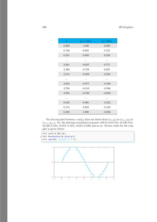
![8.3. BAR PLOT (BAR) 261
https://sites.google.com/view/arunumrao
8.3.3 Stem Plot (stem)
stem is used to plot like stems of flower. The function value is represented by
a large dot and a line is used to connect to this dot and variable point. The
return value of bar is handler ‘h’ of graphic objects. The syntax is
✞
1 >>> h=stem (x, f(x), <dot style >, <color code >)
✌
✆
If ‘dot style’ argument is omitted, then default line style is “-” and default dot
style is “o”. If ‘color code’ argument is omitted the default color code is “b”
(blue). Line styles can be change by setting “linespec” argument and color can
be changed by setting “color”. The first char of color name is used as color
code. For example “r” for “red” etc.
✞
1 >>> x=1:0.5:10;
>>> h=stem (x,sin(x),"filled")
3 >>> set(h,"color","r")
>>> set (h, " basevalue ", -1)
✌
✆
−1
0
1
−1 0 1 2 3 4 5 6 7
8.3.4 Pareto Plot (pareto)
Pareto diagrams is that the majority of an effect is due to a small subset of the
causes, so for quality improvement the first few (as presented on the diagram)
contributing causes to a problem usually account for the majority of the result.
Thus, targeting these “major causes” for elimination results in the most cost-
effective improvement scheme. The data are passed as x and y respectively for
ordinate & abscissa. If ‘y’ is absent, then the abscissa are assumed to be ‘1’ :
length (x). ‘y’ can be a string array, a cell array of strings or a numerical vector.
Example is
✞
>>> x={"a","b","c","d"};
2 >>> y=[1 ,2 ,3 ,4];
>>> pareto(y,x)
✌
✆](https://image.slidesharecdn.com/notesonoctave-cloneofmatlab-02of02byarunumrao-211010171923/85/Notes-for-GNU-Octave-Numerical-Programming-for-Students-02-of-02-by-arun-umrao-111-320.jpg)
![262 2D-Graphics
The output shall be seen in the graphics window.
8.4 Contour Plot (contour)
contour plots the contour lines of a function z = f(x, y, c) in three dimensional
planes. The syntax used for contour is
✞
1 >>> [c, h]= contour(x,y,z, <style >)
✌
✆
Here ‘c’ is 2 × n matrix containing the contour lines and ‘h’ is handler of figure
object. Contours are those lines who represents the equal heights from the base
line. Each contour has unique color and legends. In Octave, height of contour
is represented by
z = f(x, y)
Here, z is height of contour at coordinate (x, y). In the plot given below, contour
z = 1 is shown.
x
y
z
z = 1
When this contour is seen from z axis, it will looked like
x
y
bcb
z
z = 1
In Octave, contour function accepts three or more arguments, in which first
two arguments construct xy grid. Both x and y are one dimensional vectors of
size k. These two vectors construct a matrix of k ×k grid. The grid coordinates
(x, y) are constructed by these two vectors as shown in the following figure.](https://image.slidesharecdn.com/notesonoctave-cloneofmatlab-02of02byarunumrao-211010171923/85/Notes-for-GNU-Octave-Numerical-Programming-for-Students-02-of-02-by-arun-umrao-112-320.jpg)


![266 2D-Graphics
Now draw green lines by connecting each node (including major unit nodes,
i.e. ticks node and minor unit nodes, i.e. subticks nodes) whose value falls [3, 5)
(lower bound rule). This contour line is shown in the following graph.
0
1
2
3
4
5
0 1 2 3 4 5
x
y
1
1
1
1
1
3
3
3
3
3
5
5
5
5
5
7
7
7
7
7
9
9
9
9
9
By this way we can draw other contour lines. This method is used here to
explain, how contour lines are selected to plot the contour plot. There may be
different techniques to select the contour levels.
✞
1 >>> x = -2:0.25:2;
>>> y = x;
3 >>> z = x’* y;
>>> [c, h]= contour (x, y, z, -2:0.25:2);
✌
✆
8.4.1 Function Contour Plot (ezcontour)
It plots contour lines of a function f. Function f has two variables.
f(x, y) = 0
Function is calculated over the meshed domain −2π < x < 2π and −2π < y <
2π with 60 × 60 in the mesh. The syntax of this function is
✞
>>> h=ezcontour (f, [<domain >], n)
✌
✆
Here ‘domain’ is the limit range withing which points will be calculated. It may
be 2 or 4 elements vector. In two elements vector, first element is for minimum
value of x and y and second element is for maximum value of x and y. In
four element vector first two elements are for minimum and maximum values](https://image.slidesharecdn.com/notesonoctave-cloneofmatlab-02of02byarunumrao-211010171923/85/Notes-for-GNU-Octave-Numerical-Programming-for-Students-02-of-02-by-arun-umrao-116-320.jpg)
![8.4. CONTOUR PLOT (CONTOUR) 267
https://sites.google.com/view/arunumrao
of x while next two elements are for minimum and maximum values of y. In
absence of limits, two element limit vector (−2π < x|y < 2π) is used as default.
Argument ‘n’ is a scalar quantity that determines the number of points to be
used during the calculation of function value for each dimension. Default value
of ‘n’ is ‘60’. For example
✞
1 >>> ezcontour (@(x, y) x - y .^ 2 - 1)
✌
✆
With limits
✞
1 >>> ezcontour (@(x, y) x - y .^ 2 - 1, [0, 2*pi])
✌
✆
Using number of plot points
✞
1 >>> subplot (1, 2, 1);
>>> ezcontour (@(x, y) x - y .^ 2 - 1, [0, 2*pi], 5)
3 >>> subplot (1, 2, 2);
>>> ezcontour (@(x, y) x - y .^ 2 - 1, [0, 2*pi], 10)
✌
✆
Four element domain vector gives
✞
>>> ezcontour (@(x, y) x - y .^ 2 - 1, [0, 2*pi , -2*pi ,
2*pi])
✌
✆
8.4.2 Parametric Contour Plot (ezcontourf)
It plots contour lines of a function f and fills area between two consecutive
contour lines. Function f has two variables.
f(x, y) = 0
Function is calculated over the meshed domain −2π < x < 2π and −2π < y <
2π with 60 × 60 in the mesh. The syntax of this function is
✞
1 >>> h=ezcontourf (f, [<domain >], n)
✌
✆
Handel ‘h’ is returned graphic objects for body, arrow and marker. Here ‘do-
main’ is the limit range withing which points will be calculated. It may be 2 or
4 elements vector. In two elements vector, first element is for minimum value of
x and y and second element is for maximum value of x and y. In four element
vector first two elements are for minimum and maximum values of x while next
two elements are for minimum and maximum values of y. In absence of limits,
two elements limit vector (−2π < x|y < 2π) is used as default. Argument ‘n’
is a scalar quantity that determines the number of points to be used during the
calculation of function value for each dimension. For example
✞
1 >>> ezcontourf (@(x, y) x - y .^ 2 - 1)
✌
✆](https://image.slidesharecdn.com/notesonoctave-cloneofmatlab-02of02byarunumrao-211010171923/85/Notes-for-GNU-Octave-Numerical-Programming-for-Students-02-of-02-by-arun-umrao-117-320.jpg)
![268 2D-Graphics
With limits
✞
1 >>> ezcontourf (@(x, y) x - y .^ 2 - 1,[0,2* pi])
✌
✆
Using number of plot points
✞
1 >>> subplot (1, 2, 1);
>>> ezcontourf (@(x, y) x - y .^ 2 - 1,[0,2* pi],5)
3 >>> subplot (1, 2, 2);
>>> ezcontourf (@(x, y) x - y .^ 2 - 1,[0,2* pi ],10)
✌
✆
Four element domain vector gives
✞
>>> ezcontourf (@(x, y) x - y .^ 2 - 1,[0,2* pi ,-2*pi ,2*pi])
✌
✆
8.4.3 Parametric Polar Plot (ezpolar)
It plots polar plot of a function f. Function f has one variable.
f(x) = 0
Function is calculated over the meshed domain 0 < x < 2π with 60 points . The
syntax of this function is
✞
1 >>> h=ezpolar (@(x) f(x)=0,[< domain >],n)
✌
✆
Here ‘domain’ is the limits range withing which points will be calculated. It is
2 elements vector. In two elements vector, first element is for minimum value
of x and second element is for maximum value of x. In absence of limits, two
element limit vector (0 < x < 2π) is used as default. Argument ‘n’ is a scalar
quantity that determines the number of points to be used during the calculation
of function values for each dimension. Default value of ‘n’ is ‘60’. For example
✞
1 >>> ezpolar (@(x) 1 + sin(x))
✌
✆
0
0
1
1 30
60
90
120
150
180
210
240
270
300
330
360
With limits](https://image.slidesharecdn.com/notesonoctave-cloneofmatlab-02of02byarunumrao-211010171923/85/Notes-for-GNU-Octave-Numerical-Programming-for-Students-02-of-02-by-arun-umrao-118-320.jpg)
![8.4. CONTOUR PLOT (CONTOUR) 269
https://sites.google.com/view/arunumrao
✞
1 >>> ezpolar(@(x) 1 + sin(x) ,[0,2* pi])
✌
✆
0
0
1
1 30
60
90
120
150
180
210
240
270
300
330
360
Using number of plot points
✞
1 >>> subplot (2, 2, 1);
>>> ezpolar(@(x) 1 + sin(x) ,[0,2* pi],5)
3 >>> subplot (2, 2, 2);
>>> ezpolar(@(x) 1 + sin(x) ,[0,2* pi ],10)
5 >>> subplot (2, 2, 3);
>>> ezpolar(@(x) 1 + sin(x) ,[0,2* pi ],20)
7 >>> subplot (2, 2, 4);
>>> ezpolar(@(x) 1 + sin(x) ,[0,2* pi ],50)
✌
✆
0
0
1
1 30
60
90
120
150
180
210
240
270
300
330
0
0
1
1 30
60
90
120
150
180
210
240
270
300
330
0
0
1
1 30
60
90
120
150
180
210
240
270
300
330
0
0
1
1 30
60
90
120
150
180
210
240
270
300
330](https://image.slidesharecdn.com/notesonoctave-cloneofmatlab-02of02byarunumrao-211010171923/85/Notes-for-GNU-Octave-Numerical-Programming-for-Students-02-of-02-by-arun-umrao-119-320.jpg)


![8.8. QUIVER PLOT (QUIVER) 273
https://sites.google.com/view/arunumrao
automatically. If ‘labels’ argument is omitted then percentage fraction is placed
in place of label otherwise label value is put.
✞
1 >>> th = [5 ,12 ,28 ,75];
>>> exp= [0,0,0,0];
3 >>> pie(th ,exp)
✌
✆
63%
4%
10%
23%
✞
1 >>> th = [5 ,12 ,28 ,75];
>>> exp= [1 ,10 ,1 ,5];
3 >>> pie(th ,exp)
✌
✆
With ‘label’ array
✞
1 >>> th = [5 ,12 ,28 ,75];
>>> exp= [1,1,1,1];
3 >>> label= {"A","B","C","D"};
>>> pie(th ,exp ,label)
✌
✆
8.8 Quiver Plot (quiver)
Plot the (u, v) components of a vector field in an (x, y) mesh grid. If the grid
is uniform, you can specify x and y as vectors. The syntax is
✞
>>> quiver(x, y, f(x), f(y), <format >)
✌
✆
Example is
✞
1 >>> [x, y] = meshgrid (1:2:20) ;
>>> h = quiver (x, y, sin (2* pi*x/10) , sin (2*pi*y/10) );
3 >>> set (h, " maxheadsize ", 0.33);
✌
✆
“maxheadsize” is used to control the size of vector head. Three dimensional
quiver plot can be obtained by using syntax](https://image.slidesharecdn.com/notesonoctave-cloneofmatlab-02of02byarunumrao-211010171923/85/Notes-for-GNU-Octave-Numerical-Programming-for-Students-02-of-02-by-arun-umrao-123-320.jpg)

![8.11. GEOMETRIC PLOT 275
https://sites.google.com/view/arunumrao
✞
1 >>> phi = 0 : 1 : 1;
>>> h = area (sin (phi), cos (phi))
✌
✆
0
1
2
0 1 2 3 4
Another example is
✞
>>> x = 0 : 0.1 : 1;
2 >>> area (x, x .* x)
✌
✆
8.11 Geometric Plot
It is used for plotting geometrical objects.
8.11.1 Cylindrical Plot (cylinder)
cylinder function plots a function in plane of cylindrical coordinates. Cylindrical
coordinate equivalent to Cartesian coordinate system are given by
x = ρ cos θ
y = ρ sin θ
z = z
It uses mesh function internally. It uses x, y value for radius vector and z as
height. The radius ‘r’ must be at least two step vector. The ‘r’ may be like
r = a : incr : b or r = [a, b, c]. The syntax of this function is
✞
>>> [x, y, z]= cylinder (r, n)
✌
✆
It returns three dimensional matrix vectors. These vectors can be used for mesh
plot.
✞
1 >>> subplot (1, 2, 1)
>>> [x, y, z] = cylinder (10: -1:5 , 50);
3 >>> surf (x, y, z);
>>> subplot (1,2,2)
5 >>> [x, y, z] = cylinder (10: -1:0 , 50);
>>> surf (x, y, z);
✌
✆](https://image.slidesharecdn.com/notesonoctave-cloneofmatlab-02of02byarunumrao-211010171923/85/Notes-for-GNU-Octave-Numerical-Programming-for-Students-02-of-02-by-arun-umrao-125-320.jpg)
![276 3D-Graphics
8.11.2 Sphere Plot (sphere)
sphere plots a function in a plane of spherical coordinates. Spherical coordinate
system equivalent to Cartesian coordinate system are given by
x = r sin θ cos ϕ
y = r sin θ sin ϕ
z = r cos θ
It uses mesh function internally. Number of radius point is used for radius
vector. The syntax of sphere function is
✞
>>> [x, y, z]= sphere(n)
✌
✆
It returns three dimensional matrix vectors. Example is
✞
1 >>> subplot (1, 2, 1)
>>> sphere (50) ;
3 >>> subplot (1, 2, 2)
>>> sphere (100);
✌
✆](https://image.slidesharecdn.com/notesonoctave-cloneofmatlab-02of02byarunumrao-211010171923/85/Notes-for-GNU-Octave-Numerical-Programming-for-Students-02-of-02-by-arun-umrao-126-320.jpg)
![9.1. MESH PLOT 277
https://sites.google.com/view/arunumrao
93D-Graphics
To plot 3-dimensional plot we use following functions.
9.1 Mesh Plot
Before starting grid plot, first we know the following definitions.
9.1.1 Mesh Grid (meshgrid)
meshgrid returns three dimensional matrix when three arguments are supplied
to it. It returns a two dimensional matrix corresponding to x and y coordinates
of a mesh. If y is omitted, then it is assumed to be the same as x, and z is
assumed the same as y. Both x and y are one dimensional vectors of size k.
These two vectors construct a matrix of k × k grid. The grid coordinates (x, y)
are constructed by these two vectors as shown in the following figure.
x
y
z
b
(0, 0) b
(1, 0) b
(2, 0) b
(3, 0) b
(4, 0)
b
(0, 1) b
(1, 1) b
(2, 1) b
(3, 1) b
(4, 1)
b
(0, 2) b
(1, 2) b
(2, 2) b
(3, 2) b
(4, 2)
b
(0, 3) b
(1, 3) b
(2, 3) b
(3, 3) b
(4, 3)
b
(0, 4) b
(1, 4) b
(2, 4) b
(3, 4) b
(4, 4)
This returns a matrix of size k × k which is known as mess-grid. The syntax
of this function is
✞
>>> [xx , yy , zz] = meshgrid (x, y, z);
✌
✆
9.1.2 n-dimensional Grid (ngrid)
ngrid returns ‘n’ dimensional matrix when ‘n’ arguments are supplied to it.
✞
1 >>> [y1 , y2 , ..., yn] = ngrid(x1 , x2 , ..., xn);
✌
✆
9.1.3 View Point (view)
view sets the view point for a mesh or surface plot. The syntax of this function
is](https://image.slidesharecdn.com/notesonoctave-cloneofmatlab-02of02byarunumrao-211010171923/85/Notes-for-GNU-Octave-Numerical-Programming-for-Students-02-of-02-by-arun-umrao-127-320.jpg)

![9.1. MESH PLOT 279
https://sites.google.com/view/arunumrao
Larger the number of plotpoints, smaller the surface facet and fine appear-
ance of the surface mesh.
x
y
z
b
b
b
b
b b
b
b
b
b
b
b
b
b
b b b
b
b
b
b
b
b
b
b
b b
b
b
b
b
b
b
b
b
b b
b
b
b
b
b
b
b
b
b b b
b
b
b
b
b
b
b
b
b b
b
b
b
b
b
b
b
b
b b
b
b
b
b
b
b
b
b
b b b
b
b
b
b
b
b
b
b b b
b
b
b
b
b
b
b
b
b b
b
✞
1 >>> x=[0:0.3:2* pi];
>>> y=[0:0.3:2* pi];
3 >>> z=sin(x’)*cos(y);
>>> mesh (x, y, z);
✌
✆
The density of mesh lines depends on the values of ‘x’ and ‘y’. See the output
of the following example
✞
>>> x=[0:0.2:2* pi];
2 >>> y=[0:0.2:2* pi];
>>> z=sin(x’)*cos(y);
4 >>> mesh (x, y, z);
✌
✆
For different plot densities, multiple plots are plotted in same window as shown
in the following figure.
✞
>>> subplot (1, 2, 2);
2 >>> x=[0:0.3:2* pi];
>>> y=[0:0.3:2* pi];
4 >>> z=sin(x’)*cos(y);
>>> mesh (x, y, z);
6 >>> subplot (1, 2, 2);
>>> x=[0:0.2:2* pi];
8 >>> y=[0:0.2:2* pi];
>>> z=sin(x’)*cos(y);
10 >>> mesh (x, y, z);
✌
✆
9.1.5 Parametric Surface Plot (ezmesh)
ezmesh plots surface plot of a function (say parametric function plot). Its syntax
is similar to mesh function. Only method of computation is varied.](https://image.slidesharecdn.com/notesonoctave-cloneofmatlab-02of02byarunumrao-211010171923/85/Notes-for-GNU-Octave-Numerical-Programming-for-Students-02-of-02-by-arun-umrao-129-320.jpg)
![280 3D-Graphics
✞
>>> fx = @(x, t) cos(x) .*(1 + cos (t));
2 >>> fy = @(x, t) sin(x) .*(1 + cos (t));
>>> fz = @(x, t) sin(t) ;
4 >>> subplot (1,2,1)
>>> ezmesh (fx , fy , fz , [0, 10*pi], 20);
6 >>> subplot (1,2,2)
>>> ezmesh (fx , fy , fz , [0, 10*pi], 50);
✌
✆
9.2 Thee Dimensional Plot (plot3d)
This function is used to plot a function in three dimensional axes. It is similar
to the ‘mesh’ function. It uses the relation z = f(x, y). i.e. at first a mesh grid
is created for each coordinate (x, y) by using the function. The result is called
z. Now a three dimensional plot is drawn by using function plot3d(). In Octave,
plot3d function accepts three or more arguments, in which first two arguments
construct xy grid. Both x and y are one dimensional vectors of size k. These
two vectors construct a matrix of k × k grid. The grid coordinates (x, y) are
constructed by these two vectors as shown in the following figure.
x
y
z
b
(0, 0) b
(1, 0) b
(2, 0) b
(3, 0) b
(4, 0)
b
(0, 1) b
(1, 1) b
(2, 1) b
(3, 1) b
(4, 1)
b
(0, 2) b
(1, 2) b
(2, 2) b
(3, 2) b
(4, 2)
b
(0, 3) b
(1, 3) b
(2, 3) b
(3, 3) b
(4, 3)
b
(0, 4) b
(1, 4) b
(2, 4) b
(3, 4) b
(4, 4)
The z value is either computed by using any function or it is user’s input. z
is a matrix of size k × k, in which each value of z is for each grid node (x, y).
x
y
z
bb
z00
b
b
z10
b
b
z20
b
b
z30
b
b
z40
b
b
z01
b
b
z11
b
b
z21
b
b
z31
b
b
z41
b
b
z02 b
b
z12
b
b
z22
b
b
z32
b
b
z42
b
b
z03
bb
z13
b
b
z23
b
b
z33
b
b
z43
b
b
z04
b
b
z14
b
b
z24
b
b
z34
b
b
z44
Now connect the zij from its neighbouring z. Four neighbouring z nodes
form a facet of the 3D surface. The mesh thus form is three dimensional plot
of the given function.](https://image.slidesharecdn.com/notesonoctave-cloneofmatlab-02of02byarunumrao-211010171923/85/Notes-for-GNU-Octave-Numerical-Programming-for-Students-02-of-02-by-arun-umrao-130-320.jpg)
![9.3. SURFACE PLOT 281
https://sites.google.com/view/arunumrao
x
y
z
b
b
b
b
b
b
b
b b
b
b
b
b
b
b
b
b
b
b
b
b
b
b
b b
Larger the number of plotpoints, smaller the surface facet and fine appear-
ance of the surface mesh.
x
y
z
b
b
b
b
b b
b
b
b
b
b
b
b
b
b b b
b
b
b
b
b
b
b
b
b b
b
b
b
b
b
b
b
b
b b
b
b
b
b
b
b
b
b
b b b
b
b
b
b
b
b
b
b
b b
b
b
b
b
b
b
b
b
b b
b
b
b
b
b
b
b
b
b b b
b
b
b
b
b
b
b
b b b
b
b
b
b
b
b
b
b
b b
b
✞
1 >>> x = y = -5:0.5:5;
>>> [xx , yy] = meshgrid (x, y);
3 >>> z = sqrt (xx .^ 2 + yy .^ 2);
>>> zz = sin(z) ./ z;
5 >>> plot3d(xx , yy , zz);
✌
✆
9.3 Surface Plot
surf function is used to plot the surface in 3-dimension. It is similar to the mesh
function except that it fill the grad area with tension colors.
✞
1 >>> x = y = -5:0.5:5;
>>> [xx , yy] = meshgrid (x, y);
3 >>> z = sqrt (xx .^ 2 + yy .^ 2);
>>> zz = sin(z) ./ z;
5 >>> surf (xx , yy , zz);
✌
✆
9.3.1 Parametric Surface Plot (ezsurf)
It plots the surface plot to given parametric functions. Its syntax is](https://image.slidesharecdn.com/notesonoctave-cloneofmatlab-02of02byarunumrao-211010171923/85/Notes-for-GNU-Octave-Numerical-Programming-for-Students-02-of-02-by-arun-umrao-131-320.jpg)
![282 3D-Graphics
✞
1 >>> h=ezsurf(fx , fy , fz , <domain >, n)
✌
✆
Here ‘domain’ is the range of calculation of function value fx, fy and fz.
Example is
✞
1 >>> fx = @(x, t) cos(x) .*(1 + cos (t));
>>> fy = @(x, t) sin(x) .*(1 + cos (t));
3 >>> fz = @(x, t) sin(t) ;
>>> subplot (1,2,1)
5 >>> ezsurf (fx , fy , fz , [0, 10*pi], 40);
>>> subplot (1,2,2)
7 >>> ezsurf(fx , fy , fz , [0, 10*pi], 50);
✌
✆
9.3.2 Surface & Contour (surfc)
surfc plots surface and contour by computing ‘z’ matrix by receiving values from
‘x’ and ‘y’ matrices of meshgrid. It is similar to mesh function.
✞
1 >>> x = y = -5:0.5:5;
>>> [xx , yy] = meshgrid (x, y);
3 >>> z = sqrt (xx .^ 2 + yy .^ 2);
>>> zz = sin(z) ./ z;
5 >>> surfc(xx , yy , zz);
✌
✆
9.3.3 Surface Light (surfl)
surfl plot a lighted surface by computing ‘z’ matrix by receiving values from ‘x’
and ‘y’ matrices of meshgrid. The syntax of this function is
✞
1 >>> surfl(x, y, z, <light >, <material strength >);
✌
✆
‘z’ matrix is computed by using the relation
z = f(x, y)
The light direction can be specified using ‘light’. It can be given as 2-element
vector as [azimuth, elevation] in degrees or as 3-element vector [lx, ly, lz]. The
default value is rotated 45 counter-clockwise from the current view. The ma-
terial properties of the surface can specified using a 4-element vector P = [AM
D SP exp] which defaults to p = [0.55 0.6 0.4 10]. Here “AM” is strength of
ambient light, “D” is strength of diffuse reflection, “SP” is strength of specular
reflection and “EXP” is specular exponent.
✞
1 >>> x = y = -5:0.25:5;
>>> [xx , yy] = meshgrid (x, y);](https://image.slidesharecdn.com/notesonoctave-cloneofmatlab-02of02byarunumrao-211010171923/85/Notes-for-GNU-Octave-Numerical-Programming-for-Students-02-of-02-by-arun-umrao-132-320.jpg)
![9.4. PLOT ANNOTATIONS 283
https://sites.google.com/view/arunumrao
3 >>> z = sqrt (xx .^ 2 + yy .^ 2);
>>> zz = sin (z) ./ z;
5 >>> vw =[30 ,30];
>>> MA =[0.55 0.6 0.4 10];
7 >>> surfl (xx , yy , zz ,vw ,MA);
✌
✆
9.4 Plot Annotations
Plot annotations are used to enhance the meaning and presentation of the plot.
9.4.1 Title (title)
title function is used to add title to the plot.
✞
1 >>> x = -10:0.1:10;
>>> plot (x, sin (x));
3 >>> title ("sin(x) for x = -10:0.1:10");
✌
✆
9.4.2 X, Y & Z-axis Labels
xlabel, ylabel and zlabel functions are used to put the labels for x-axis, y-axis
and z-axis respectively. Syntax used are
✞
1 >>> h=xlabel(<text >);
>>> h=ylabel(<text >);
3 >>> h=zlabel(<text >);
✌
✆
It returns graphic object handler.
✞
1 >>> x = -10:0.1:10;
>>> plot (x, sin (x));
3 >>> h1=xlabel("x");
>>> h2=ylabel("sin(x)");
✌
✆
9.4.3 Text (text)
text function puts string at required location. Its syntax is
✞
>>> h=text (x, y, z, <text >);
✌
✆
It returns graphic object handler.
✞
1 >>> x = -10:0.1:10;
>>> plot (x, sin (x));
3 >>> h=text (1,0.25,"sin(x)");
✌
✆](https://image.slidesharecdn.com/notesonoctave-cloneofmatlab-02of02byarunumrao-211010171923/85/Notes-for-GNU-Octave-Numerical-Programming-for-Students-02-of-02-by-arun-umrao-133-320.jpg)


![286 3D-Graphics
✞
1 >>> figure(n, <property >, <value >
✌
✆
Here ‘n’ is a positive integer for identifying figure window. If ‘n’ is omitted
then automatically next figure window id is selected. Two figure window with
difference function are shown following example.
✞
1 >>> figure (10) ;
>>> fplot (@(x) x .^2, [-5, 5]);
3 >>> figure (20) ;
>>> fplot (@cos , [-5, 5]);
✌
✆
9.5.3 Print or Save a Plot
print function is used to save or print the graphics. The syntax of this function
is
✞
>>> print(<handler >,<file name >,<options >)
✌
✆
If there is not ‘handler’, current graphics is selected automatically. ‘file name’
is the name of file to be saved. In absence of ‘file name’, figure is sent to printer
for print.
✞
1 >>> fplot (@(x) sin(x) .* cos(x), [-5, 5]);
>>> h=gcf ();
3 >>> print(h,"a.jpg")
✌
✆
It saves the plot as a “a.jpg” in the current working directory. Various types of
‘options’ used in print function. The option table is
Options Value & Description
fh Specify the handle
color Value mono gives monochrome output.
solid Force all lines to be solid.
dashed Force all lines to be dashed.
portrait Portrait paper size.
landscape Landscape paper size.
rNUM Resolution of image.
loose Loose bounding box.
tight Tight bounding box.](https://image.slidesharecdn.com/notesonoctave-cloneofmatlab-02of02byarunumrao-211010171923/85/Notes-for-GNU-Octave-Numerical-Programming-for-Students-02-of-02-by-arun-umrao-136-320.jpg)
![9.5. GRAPHICS OBJECT 287
https://sites.google.com/view/arunumrao
9.5.4 Graphics Handler
The return value of a function is assigned to a handler. Handler is that object
which points to the properties and attributes of a graphics. To change the
specific key of a graphics object, value of key must be supplied by using handler.
9.5.5 Handling of Graphic’s Object
A graphics is a bundle of following sub objects.
1. root figure : The parent of all figure object. The index of root figure is
zero.
2. axes : A set of axes. This object is a child of a figure object and parent
of line, text, image etc.
3. line : A line in two or three dimension.
4. text : Text annotation.
5. image : A bitmap image.
6. surface : A three dimensional surface.
To determine whether a variable is a handle, graphics object index or figure
index we use ishandle, ishghandle and isfigure respectively. These functions
accepts object argument like:
✞
1 >>> ishandle (<handler >)
✌
✆
It returns true if object supplied to this function as its argument is a handle
object otherwise returns false. ishghandle returns true if object supplied to this
function as its argument is graphics handler otherwise returns false. Similarly
isfigure returns true if object supplied to this function as its argument is figure
handle.
✞
1 >>> h=figure (10) ;
>>> fplot (@(x) x .^2, [-5, 5]);
3 >>> ishandle (h)
✌
✆
The output is
✞
ans = 1
✌
✆](https://image.slidesharecdn.com/notesonoctave-cloneofmatlab-02of02byarunumrao-211010171923/85/Notes-for-GNU-Octave-Numerical-Programming-for-Students-02-of-02-by-arun-umrao-137-320.jpg)

![9.5. GRAPHICS OBJECT 289
https://sites.google.com/view/arunumrao
To see the specific property value, use get function like
✞
1 >>> get(<handler >, <key string >)
✌
✆
To change the figure object set function is used like
✞
1 >>> set(<handler >, <key >, <new value >)
✌
✆
Example is
✞
1 >>> fplot (@(x) x .^2, [-5, 5])
>>> h=gcf()
3 >>> get(h)
>>> set(h,"visible ","off")
✌
✆
These code will create a graphics and will put it into graphic window and then
close it.
Key Value & Description
clipping Controls the clipping.
color Color of the image. Default is [r g b].
currentaxes Position of current axis.
filename Name of graphics.
integerhandle Controls integer handle. Value is on or off.
menubar Figure menu .
parent Graphics window is parent window or not.
papertype Paper type like A3, A4 etc.
paperunits Size unit of paper type. Default is inches.
position Position of graphics.
renderer Renderer of the graphics.
renderermode Graphics rendering mode. Default is painter.
resize Resize of graphics. Default is on.
toolbar Toolbar of graphics.
units Graphics unit.
Table 9.1: Key-value of gcf () function.
These are few of the all graphics properties and their default values. To list
the all properties, use get function as explained above.](https://image.slidesharecdn.com/notesonoctave-cloneofmatlab-02of02byarunumrao-211010171923/85/Notes-for-GNU-Octave-Numerical-Programming-for-Students-02-of-02-by-arun-umrao-139-320.jpg)
![290 3D-Graphics
9.5.8 Get Current Axes Object (gca)
In each graphics window, the hierarchy arev ‘root’, ‘figure’, ‘axes’, ‘line’, ‘text’,
‘patch’, ‘surface’, ‘text’, and ‘’image’ from top level to bottom level. The root
object is at 0. This function, i.e. gca returns the index to current axes object
and assigns it to its object handler. Syntax is
✞
>>> h = gca ();
✌
✆
‘h’ is handler of axes. There are hundreds of the properties of axes which
are arranged in key-value arrangement under the axes object. To see all the
properties of axes object, use get function like
✞
1 >>> get(<handler >, <key string >)
✌
✆
get function is useful to list all properties and finding what do we want to
update. To change the requisite property of axes object set function is used like
✞
1 >>> set(<handler >, <key >, <new value >)
✌
✆
✞
1 >>> fplot (@(x) sin(x) .* cos(x), [-5, 5])
>>> h=gca ()
3 >>> get(h)
>>> set(h,"box","off")
✌
✆](https://image.slidesharecdn.com/notesonoctave-cloneofmatlab-02of02byarunumrao-211010171923/85/Notes-for-GNU-Octave-Numerical-Programming-for-Students-02-of-02-by-arun-umrao-140-320.jpg)


![298 Others
✞
1 >>> days = datenum (2014 ,12 ,12)
✌
✆
✞
ans =
735945
✌
✆
11.1.6 Date As String (datestr)
It converts string into corresponding date. The syntax is
✞
>>> str=datestr (<string >, <format >)
✌
✆
‘format’ is the option for date format output. It is “dd-mm-yyyy” or “dd-mm-
yy”. If month part has only two chars then month will be printed in numeric
format otherwise month name is return. Length of month name is equal to
the number of characters in month part. Similarly, year length is controlled by
number of characters in year part. For example
✞
1 >>> a=datestr (602154)
>>> b=datestr (602154 ,"dd -mm -yy")
3 >>> c=datestr (602154 ,"dd -mm -yyyy ")
>>> d=datestr (602154 ,"dd -m-yyyy ")
5 >>> e=datestr (602154 ,"dd -mmm -yyyy ")
✌
✆
✞
a = 21-Aug -1648
b = 21-08-48
c = 21 -08 -1648
d = 21-A -1648
e = 21-Aug -1648
✌
✆
11.1.7 Ticks As Date In Axes (datetick)
It adds date formatted tick labels to an axis of the graphical plot.
11.1.8 Date As Vector (datevec)
It returns year, month, day, hours, minutes and seconds from a date string.
✞
1 >>> [y, m, d, h, mi , s]= datevec(<date string >, <format >)
✌
✆
✞
1 >>> a = datevec (602154 ,"dd -mmm -yyyy ")
>>> b = datevec ("2014 -12 -30 ")
✌
✆](https://image.slidesharecdn.com/notesonoctave-cloneofmatlab-02of02byarunumrao-211010171923/85/Notes-for-GNU-Octave-Numerical-Programming-for-Students-02-of-02-by-arun-umrao-148-320.jpg)


![11.3. WRITING MEX MACROS 301
https://sites.google.com/view/arunumrao
✞
1 #include "mex.h"
✌
✆
and starting function node. The starting function in Octave is mexFunc-
tion like to the main function of C.
2. Now put the code structure like
✞
1 #include "mex.h"
3 void mexFunction (
int nlhs , /* Number of outputs */
5 mxArray *plhs [], /* Output arrays*/
int nrhs , /* Number of inputs */
7 const mxArray *prhs []){ /* Input arrays*/
/* mexPrintf prints the data in output stream .*/
9 mexPrintf ("Hello , It is first macro
function .!n");
}
✌
✆
mexFunction function needs four arguments to handle input and output
stream.
(a) nlhs : It is short form of Number of argument in Left Hand Side. It
represents to the output arguments.
(b) plhs : Array of returned pointer in left hand side.
(c) nrhs : It is short form of Number of argument in Right Hand Side.
It represents to the input arguments.
(d) prhs : Array of input pointer in right hand side.
The left hand side and right hand side of an equation or expression
y = ax + b
are y and x respectively. The left side is output variable of the expression,
while right hand side is expression that is being evaluated. To give a
function name to this code file, it is saved as ‘hello.c’. It means the
expressions of the file ‘hello.c’ shall be called from the function hello().
3. Now compile the file from the octave command line console or from GUI
as
✞
>>> mkoctfile --mex hello.c
✌
✆
or like as
✞
1 >>> mex(hello.c)
✌
✆](https://image.slidesharecdn.com/notesonoctave-cloneofmatlab-02of02byarunumrao-211010171923/85/Notes-for-GNU-Octave-Numerical-Programming-for-Students-02-of-02-by-arun-umrao-151-320.jpg)
![302 Others
The path of file name may be relative or absolute.
4. The function hello() can be called from Octave input stream as
✞
1 >>> hello()
✌
✆
Output shall be shown in the Octave console.
✞
Hello , It is first macro function .!
✌
✆
5. There is single entry points for a single mex-file. Expressions for a function
are defined in a separate file. A function name is actual a file name. The
mexFunctionName function is used to get the name of called function. It
is used to alter the behavior of the mex-file based on the function name.
Syntax for mexFunctionName is
✞
1 const char *nm;
nm = mexFunctionName ();
✌
✆
See the example below:
✞
# include "mex.h"
2
void mexFunction (
4 int nlhs , /* Number of outputs */
mxArray *plhs [], /* Output arrays*/
6 int nrhs , /* Number of inputs */
const mxArray *prhs []/* Input arrays*/
8 ){
const char *nm;
10 /* Get the called function name .*/
nm = mexFunctionName ();
12
/* Print the function name */
14 mexPrintf ("You say %sn", nm);
if (strcmp (nm , "hello") == 0)
16 mexPrintf ("This is first %sn", nm);
18 return;
}
✌
✆
Compile this file and call function hello like
✞
1 >>> hello()
✌
✆](https://image.slidesharecdn.com/notesonoctave-cloneofmatlab-02of02byarunumrao-211010171923/85/Notes-for-GNU-Octave-Numerical-Programming-for-Students-02-of-02-by-arun-umrao-152-320.jpg)
![11.3. WRITING MEX MACROS 303
https://sites.google.com/view/arunumrao
✞
You say hello
This is first hello
✌
✆
mex
mex function is used to compile a user written function into the Octave files. It
is equal to command-line instruction
✞
>>> mkoctfile --mex
✌
✆
mex function accepts file name as its argument. Path to file may be either
absolute or relative path. The file name exactly the function name, so it should
be properly named.
✞
1 >>> mex(hello.c)
✌
✆
The compiled function name shall be hello.
mexext
It returns the file name extension used for MEX files.
✞
1 >>> mexext()
✌
✆
11.3.2 Matrix & Array
The basic mex type of all variables is mxArray. Any object, such as a matrix,
cell array, or structure is stored in this basic type. mxArray structure stores
the name of variable, its data, data type, dimension etc. It acts like a container
or database of variables. The basic function to access the data contained in an
array is mxGetPr. In mxArray, real and imaginary parts of a complex array are
stored separately. Real part of data is accessed by function mxGetRe. Imagi-
nary part of data is accessed by function mxGetPi. Both of these functions are
only for use with double precision matrices. The generic functions mxGetData
and mxGetImagData perform the same operation on all matrix types. Function
mxSetPr points to the block of memory pointed by its argument. mwSize is
used to define array dimensions and the maximum number or elements, while
mwIndex is used to define indexing into arrays. mxGetNumberOfElements re-
turns the number of elements in a matrix.
✞
1 #include "mex.h"
/* Entry function */
3 void mexFunction (
int nlhs , /* Number of outputs */
5 mxArray *plhs [], /* Output arrays */](https://image.slidesharecdn.com/notesonoctave-cloneofmatlab-02of02byarunumrao-211010171923/85/Notes-for-GNU-Octave-Numerical-Programming-for-Students-02-of-02-by-arun-umrao-153-320.jpg)
![304 Others
int nrhs , /* Number of inputs*/
7 const mxArray *prhs [] /* Input arrays */
){
9 mwSize n; /* matrix width size */
/* check the required number of inputs*/
11 if (nrhs != 1)
/* show error messages if not required inputs */
13 mexErrMsgTxt (" Argument 1 must be a matrix");
/* Get number of elements in a matrix */
15 n = mxGetNumberOfElements (prhs [0]) ;
mexPrintf ("Number of elements are %dn",n);
17 }
✌
✆
Save above codes in a file, named as ‘E.c’ and compile it with mex() function.
On call of function like
✞
1 E([1 ,2;3 ,4])
✌
✆
it returns the result as shown below.
✞
Number of elements are 4;
✌
✆
Functions mxCreateDoubleMatrix, mxCreateCellArray, mxCreateSparse andmxCreateNumericArra
creates mxArray to store the respective data. Following is my code file named
“c.c”.
✞
1 /* Incluce matlab execusion header*/
#include "mex.h"
3 /* Entry function */
void mexFunction (
5 int nlhs , /* Number of outputs */
mxArray *plhs [], /* Output arrays */
7 int nrhs , /* Number of inputs*/
const mxArray *prhs [] /* Input arrays */
9 ){
mwSize n; /* matrix width size */
11 mwIndex i; /* matrix index*/
double *vri , *vro ;/* vector inputs and vector outputs */
13
/* check the required number of inputs */
15 if (nrhs != 1 || ! mxIsNumeric (prhs [0]) )
/* show error messages if not required inputs */
17 mexErrMsgTxt (" Argument 1 must be a matrix");
/* get the number of elements in input array*/
19 n = mxGetNumberOfElements (prhs [0]) ;
plhs [0] =
mxCreateNumericArray ( mxGetNumberOfDimensions(prhs [0]) ,
21 mxGetDimensions (prhs [0]) ,
mxGetClassID (prhs [0]) ,](https://image.slidesharecdn.com/notesonoctave-cloneofmatlab-02of02byarunumrao-211010171923/85/Notes-for-GNU-Octave-Numerical-Programming-for-Students-02-of-02-by-arun-umrao-154-320.jpg)
![11.3. WRITING MEX MACROS 305
https://sites.google.com/view/arunumrao
23 mxIsComplex (prhs [0]) );/* create number array */
vri = mxGetPr (prhs [0]) ;/* get vector elements as input*/
25 vro = mxGetPr (plhs [0]) ;/* get vector elements as output
*/
if (mxIsComplex (prhs [0]) ) { /* if input is as complex
number*/
27 double *vii , *vio;
vii = mxGetPi(prhs [0]) ;
29 vio = mxGetPi(plhs [0]) ;
for (i = 0; i < n; i++) {
31 /* for each element get real value*/
vro[i] = vri[i] * vri[i] - vii[i] * vii[i];
33 vio[i] = 2 * vri[i] * vii[i];/* get imaginary
part */
}
35 } else {/* otherwise */
for (i = 0; i < n; i++)
37 vro[i] = vri[i] * vri[i]; /* get square of the
element */
}
39 }
✌
✆
Compile this file using mex function and call the function like
✞
1 >>> c(<vector or matrix >)
✌
✆
For example
✞
1 >>> c([1 ,2 ,3 ,4])
✌
✆
✞
ans =
1 4 9 16
✌
✆
11.3.3 Strings
Mex-files do not make the distinction between single quoted or double quoted
strings within Octave. There is perhaps less complexity in the use of strings and
character matrices in mex-files. mxGetM and mxGetN returns the number of
rows and columns of the array mxArray. mxGetNumberOfDimensions is used
to get the dimension of the matrix.
✞
#include <string.h>
2 #include "mex.h"
4 void mexFunction (int nlhs ,
mxArray* plhs [],
6 int nrhs ,](https://image.slidesharecdn.com/notesonoctave-cloneofmatlab-02of02byarunumrao-211010171923/85/Notes-for-GNU-Octave-Numerical-Programming-for-Students-02-of-02-by-arun-umrao-155-320.jpg)
![306 Others
const mxArray* prhs []){
8 mwSize m, n;
10 if (nrhs != 1 ||
mxGetNumberOfDimensions(prhs [0]) > 2)
12 mexErrMsgTxt (" Argument 1 must be a char matrix");
14 m = mxGetM(prhs [0]) ;
mexPrintf ("Rows are %dn", m);
16 n = mxGetN(prhs [0]) ;
mexPrintf ("Columns are %dn", n);
18 }
✌
✆
Save above code in file ‘f.c’. Compile it by using function mex() and call the
function like
✞
>>> f([1 ,2;4 ,5])
✌
✆
The output is
✞
Rows are 2
Columns are 2
✌
✆
Mex files considers a character string as a vector rather than matrix. mx-
IsChar checks whether a supplied string is a character string or not. mxChar
creates a character pointer. mxGetChars is used to get the pointer of input or
output character stream.
✞
#include <string.h>
2 #include "mex.h"
4 void mexFunction (int nlhs ,
mxArray * plhs [],
6 int nrhs ,
const mxArray* prhs []){
8 mwSize m, n;
mwIndex i, j;
10 mxChar *pi , *po;
12 if (nrhs != 1 || ! mxIsChar (prhs [0])
|| mxGetNumberOfDimensions(prhs [0]) > 2)
14 mexErrMsgTxt ("Argument 1 must be a char
matrix");
16 m = mxGetM(prhs [0]) ;
mexPrintf ("Rows are %dn", m);
18 n = mxGetN(prhs [0]) ;
mexPrintf ("Columns are %dn", n);
20 pi = mxGetChars (prhs [0]) ;](https://image.slidesharecdn.com/notesonoctave-cloneofmatlab-02of02byarunumrao-211010171923/85/Notes-for-GNU-Octave-Numerical-Programming-for-Students-02-of-02-by-arun-umrao-156-320.jpg)
![11.3. WRITING MEX MACROS 307
https://sites.google.com/view/arunumrao
plhs [0] = mxCreateNumericMatrix (m, n, mxCHAR_CLASS ,
mxREAL);
22 po = mxGetChars (plhs [0]) ;
24 for (j = 0; j < n; j++)
for (i = 0; i < m; i++)
26 po[j * m + m - 1 - i] = pi[j * m + i];
}
✌
✆
Save above code in file ‘f.c’. Compile it by using function mex() and call the
function like
✞
1 >>> f(["a","b";"c","d"])
✌
✆
The output is
✞
ans =
cd
ab
✌
✆
Function mxCreateString is used to create a string. mxArrayToString is
used to create a string from array. mxCreateCharMatrixFromStrings is used to
convert an string into character matrix.
11.3.4 Cell Array
See the following example:
✞
#include "mex.h"
2
void mexFunction (int nlhs ,
4 mxArray* plhs [],
int nrhs ,
6 const mxArray * prhs []) {
mwSize n;
8 mwIndex i;
10 if (nrhs != 1 || !mxIsCell (prhs [0]) )
mexErrMsgTxt ("Argument 1 must be a cell ");
12 /* Get the number of elements */
n = mxGetNumberOfElements (prhs [0]) ;
14 /* If supplied number is greater than length of
* cell array in supplied argument then use cell
16 * array length otherwise use supplied number .*/
n = (n > nlhs ? nlhs : n);
18 /* Create new array as you want to be appear in output
console .*/
for (i = 0; i < n; i++)](https://image.slidesharecdn.com/notesonoctave-cloneofmatlab-02of02byarunumrao-211010171923/85/Notes-for-GNU-Octave-Numerical-Programming-for-Students-02-of-02-by-arun-umrao-157-320.jpg)
![308 Others
20 plhs [i] = mxDuplicateArray (mxGetCell (prhs [0], i));
}
✌
✆
In place of mxGetCell in above example we can use mxSetCell also by using the
syntax like
✞
1 void mxSetCell (mxArray *ptr , int idx , mxArray *val);
✌
✆
And use mxCreateCellArray or mxCreateCellMatrix in place of mxDuplicateAr-
ray according to syntax
✞
1 mxArray * mxCreateCellArray (int ndims , const int *dims );
mxArray * mxCreateCellMatrix (int m, int n);
✌
✆
for creating a cell array output.
11.3.5 Structures
✞
#include "mex.h"
2
void mexFunction (int nlhs ,
4 mxArray * plhs [],
int nrhs ,
6 const mxArray* prhs []) {
int i;
8 mwIndex j;
mxArray *v;
10 const char *keys [] = {"this ", "that "};
12 if (nrhs != 1 || ! mxIsStruct (prhs [0]) )
mexErrMsgTxt (" expects struct");
14
for (i = 0; i < mxGetNumberOfFields (prhs [0]) ; i++)
16 for (j = 0; j < mxGetNumberOfElements (prhs [0]) ;
j++) {
mexPrintf ("field %s(%d) = ",
mxGetFieldNameByNumber(prhs [0], i), j);
18 v = mxGetFieldByNumber (prhs [0], j, i);
mexCallMATLAB (0, NULL , 1, &v, "disp ");
20 }
22 v = mxCreateStructMatrix (2, 2, 2, keys );
24 mxSetFieldByNumber (v, 0, 0, mxCreateString ("this1"));
mxSetFieldByNumber (v, 0, 1, mxCreateString ("that1"));
26 mxSetFieldByNumber (v, 1, 0, mxCreateString ("this2"));
mxSetFieldByNumber (v, 1, 1, mxCreateString ("that2"));
28 mxSetFieldByNumber (v, 2, 0, mxCreateString ("this3"));](https://image.slidesharecdn.com/notesonoctave-cloneofmatlab-02of02byarunumrao-211010171923/85/Notes-for-GNU-Octave-Numerical-Programming-for-Students-02-of-02-by-arun-umrao-158-320.jpg)
![11.4. STANDALONE PROGRAMS 309
https://sites.google.com/view/arunumrao
mxSetFieldByNumber (v, 2, 1, mxCreateString ("that3"));
30 mxSetFieldByNumber (v, 3, 0, mxCreateString ("this4"));
mxSetFieldByNumber (v, 3, 1, mxCreateString ("that4"));
32
if (nlhs )
34 plhs [0] = v;
}
✌
✆
11.3.6 Calling Other Functions
We can call inbuilt Octave function through mex files by using the function mex-
CallMATLAB. The calling mex function needs input arguments in which first
argument must be a Octave named function. The named function is executed
with mexCallMATLAB function.
✞
1 #include "mex.h"
3 void mexFunction (int nlhs ,
mxArray* plhs [],
5 int nrhs ,
const mxArray * prhs []) {
7 char *str;
mexPrintf ("Calling a function !n");
9 mexPrintf ("Here are %d inputs and %d outputsn", nrhs ,
nlhs );
/* Check first argument is a function string .*/
11 if (nrhs < 1 || !mxIsString (prhs [0]) )
mexErrMsgTxt ("Argument 1 must be a function name ");
13 /* Convert array to string .*/
str = mxArrayToString (prhs [0]) ;
15 mexPrintf ("I’m going to call the function %sn", str);
/* Call the function using mexCallMATLAB function . */
17 mexCallMATLAB (nlhs , plhs , nrhs - 1, ( mxArray *) prhs +
1, str);
mxFree(str);
19 }
✌
✆
Any called function must be freed by using mxFree function.
11.4 Standalone Programs
The Octave library ‘liboctave.a’ or ‘liboctave.so’ have classes which define the
data type, indices, arrays and matrices. We can access them in standalone
programs. The basic structure of the standalone program is
✞
1 #include <xx.h>
#include <octave/oct.h>](https://image.slidesharecdn.com/notesonoctave-cloneofmatlab-02of02byarunumrao-211010171923/85/Notes-for-GNU-Octave-Numerical-Programming-for-Students-02-of-02-by-arun-umrao-159-320.jpg)

![312 Others
✞
1 #include <iostream >
#include <octave/oct.h>
3 #include <octave/octave.h>
#include <octave/parse.h>
5 #include <octave/interpreter .h>
/*C or C++ function starting point*/
7 int main (void ){
string_vector argv (2);
9 argv (0) = "embedded ";
argv (1) = "-q";
11 /* Octave main function . It is similar to *
*main (int argc , char ** argv ) function . *
13 *Third argument of octave_main is true / *
*false of embedded type programs . */
15 octave_main (2, argv .c_str_vec (), 1);
17 /* Number of inputs */
int n = 2;
19 /* or we can use */
// octave_idx_type n = 2;
21
/* The input variable list */
23 octave_value_list in;
25 for (int i = 0; i < n; i++)
in(i) = octave_value (10 * (i + 2));
27
/* The output variable list and call *
29 *interpreter function feval(). */
octave_value_list out = feval ("gcd", in , 1);
31
if (! error_state && out.length () > 0)
33 std :: cout << "GCD of ["
<< in (0).int_value ()
35 << ", "
<< in (1).int_value ()
37 << "] is " << out (0).int_value ()
<< std:: endl ;
39 else
std :: cout << " invalidn";
41
clean_up_and_exit (0);
43 }
✌
✆
✞
GCD of [20, 30] is 10
✌
✆
In case of we are using only built-in functions which are to be called from a C++
standalone program, then we do not need interpreter, i.e. call of named function](https://image.slidesharecdn.com/notesonoctave-cloneofmatlab-02of02byarunumrao-211010171923/85/Notes-for-GNU-Octave-Numerical-Programming-for-Students-02-of-02-by-arun-umrao-162-320.jpg)


Ad
More Related Content
What's hot (20)
Similar to Notes for GNU Octave - Numerical Programming - for Students - 02 of 02 by arun umrao (20)


Ad
More from ssuserd6b1fd (20)


Ad
Recently uploaded (20)


Notes for GNU Octave - Numerical Programming - for Students - 02 of 02 by arun umrao
- 1. 2.2. GLOBAL VARIABLE 151 https://sites.google.com/view/arunumrao ✞ x = { a = 1 a1 = 2 a2 = 3 } ✌ ✆ Since variable names may only contain letters, digits and underscores, genvar- name replaces any sequence of disallowed characters with an underscore. Also, variables may not begin with a digit; in this case an underscore is added before the variable name. Variable names beginning and ending with two underscores (“ ”) are valid but they are used internally by Octave and should generally be avoided, therefore genvarname will not generate such names. genvarname will also make sure that returned names do not clash with keywords such as “for” and “if”. A number will be appended if necessary. Note, however, that this does not include function names, such as “sin”. Such names should be included in avoid if necessary. 2.2 Global Variable A variable that has been declared as global may be accessed from within a function body without having to pass it as a formal parameter. A variable is set global by using global statement. Three variables ‘x’, ‘y’ and ‘z’ with ‘y’=1 are set as global variable in following example. ✞ >>> global x y=1 z; ✌ ✆ Global variable can be assigned only once. If same variable is required to use as global variable again, first use ✞ 1 >>> clear <global variable > ✌ ✆ or ✞ 1 >>> clear all ✌ ✆ A variable set global outside a function can not be assigned a value from the body of the function. But it just copy the value to global variable for use inside the function. ✞ 1 >>> global x; # global variable x >>> function f(x) 3 >>> x=1; # assigned value 1 withing function body >>> x # call variable within function body , prints 1 5 >>> endfunction >>> f() # call function 7 >>> x # call global variable , prints [](0 x0) for null value ✌ ✆
- 2. 152 Variable ✞ x = 1 x = [](0 x0) ✌ ✆ 2.2.1 Is Variable Global isglobal is used to find whether a variable is global or not. It returns ‘true’ if variable is global otherwise ‘false’. ✞ >>> global x; # global variable x 2 >>> isglobal ("x") ✌ ✆ ✞ ans = 1 ✌ ✆ 2.3 Persistant Of a Variable A variable that has been declared persistent within a function will retain its con- tents in memory between subsequent calls to the same function. The difference between persistent variables and global variables is that persistent variables are local in scope to a particular function and are not visible elsewhere. ✞ 1 >>> global x=1; # global scope; can be called or copy anywhere >>> isglobal ("x") 3 >>> function f(y); >>> y=2; #local scope; within the function body 5 >>> endfunction ✌ ✆ ✞ ans = 1 ✌ ✆ 2.3.1 Clear Symbol From Table (clear) Delete the names matching the given patterns from the symbol table. The pattern may contain the following special characters: 1. ‘?’ : Match any single character. 2. ‘*’ : Match zero or more characters. 3. ‘[ ¡list¿ ]’ : Match the list of characters specified by list. If the first character is ‘!’ or ‘ˆ’ then matching of all characters is performed excepting those specified by a list. For example, the pattern [a-zA-Z]’ will match all lower and upper case alphabetic characters. For example
- 3. 2.3. PERSISTANT OF A VARIABLE 153 https://sites.google.com/view/arunumrao ✞ 1 >>> clear foo b*r ✌ ✆ clears the name ‘foo’ and all names that begin with the letter ‘b’ and end with the letter ‘r’. If clear is called without any arguments, all user-defined variables (local and global) are cleared from the symbol table. 2.3.2 Show Files in Directory (what) what command is used to find all the Octave files in the directory. Syntax is ✞ 1 >>> what (<dir name >) ✌ ✆ If ‘dir name’ is empty, it returns the list of Octave files from the current path. 2.3.3 Function Name Type (which) It displays the type of each name. If name is defined from a function file, the full name of the file is also displayed. 2.3.4 Scope of Variable (who) who returns the scope of variable supplied by pattern. For example ✞ 1 >>> global x; >>> what ("x") ✌ ✆ ✞ Variables in the current scope: x ✌ ✆ Or ✞ >>> global x; 2 >>> who("global") ✌ ✆ ✞ Global variables : x ✌ ✆ 2.3.5 Exit From Loop (exist) exist returns whether the variable, function, file or director specifiend as argu- ment to the function are exist or not exist in the sytem. The syntax of this function is ✞ >>> exist(<name >, <type >) ✌ ✆
- 4. 154 Functions There are four types of ‘type’ values. Type Description “var” Check only for variables “builtin” Check only for built-in functions “file” Check only for files “dir” Check only for directories Example is ✞ 1 >>> exist("meaning","var") ✌ ✆ ✞ ans = 0 ✌ ✆
- 5. 3.1. FUNCTION 155 https://sites.google.com/view/arunumrao 3Functions Octave is written in ‘C’ and ‘C++’. Unlike ‘C++’ Octave does not required pre-definition of variable. Variables are automatically converted into integer, character etc forms according to the values passed to them. In other words, a value is assigned to a variable by juggling. If a variable ‘a’ is being added with ‘2’ then the variable ‘a’ would be considered as an integer type variable. But if it is to be added with ‘2.00202201220215’ then variable ‘a’ will be considered as an long type variable. In summary type of a variable is considered as it is being used. Each statement performed internally should be terminated by ‘;’. The statement whose result would be display in output window should not end with ‘;’. Statements, strings and variables are grouped inside a parenthesis brackets, ie ‘(’ ... ‘)’. Generally octave uses following code conventions. According to the Code Conventions for the Octave Programming Language it is recommended: 1. Start each statement on a new line. 2. Write no more than one simple statement per line. 3. Break compound statements over multiple lines. Following example uses two integers 2, 3 & ‘;’ and prints their result at output window. ✞ 1 /* Without pre -identification of * *variable and terminated by ’;’*/ 3 >>> a=2; /* Without pre -identification of * 5 *variable and terminated by ’;’*/ >>> b=3; 7 /* sum of two variables is called * *line does not terminated by ’;’*/ 9 >>> a+b ✌ ✆ ✞ ans = 5 ✌ ✆ If result of an operation is not assigned to a variable, then result is automatically assigned to ‘ans’ variable. 3.1 Function Function, in computer science is a set of instructions. This set of instruction is collectively called a script or code. Codes inside the function are not executed until unless function is not called. Some times more than one functions or com- mands are successively used for a specific purpose. The re-usability of these sets
- 6. 156 Functions of functions or commands is very problematic. Hence these set of functions or commands are put inside a new function defined by user. Now this new defined function can be used as and when required. Octave is a strong language. It supports grouping of expressions. A group block started with reserved keyword and ended with the same keyword prefixed with ‘end’. ✞ 1 function f(x) <expression or codes > 3 endfunction ✌ ✆ ✞ 1 for <condition > <expression or codes > 3 endfor ✌ ✆ Octave has strong commenting support. Commenting are those lines which are inserted inside the program code to make it better understandable. Single line commenting is made with ‘#’ or ‘%’ symbols at the beginning of a line. These comments are just skipped by compilers and are not executed as part of the program. Entire block of lines can be commented by enclosing the lines between matching ‘#{ and ‘#} or ‘%{ and ‘%} markers. ✞ 1 #Beginning of a function function f(x) 3 <expression or codes > #{ 5 This block shall be executed when function f(x) is called. 7 #} endfunction ✌ ✆ 3.1.1 Defining A Functions In its simplest form, the definition of a function named name looks like this: ✞ >>> function <name > 2 >>> <body > >>> endfunction ✌ ✆ A function name should be a valid name. A valid function name contains letters, digits and underscores. A function name should not starting with a digit. In octave, the parameters are passed to a function as shown in following synopsis. ✞ 1 >>> function <name > (<arg -list >) >>> <body > 3 >>> endfunction ✌ ✆
- 7. 3.1. FUNCTION 157 https://sites.google.com/view/arunumrao A function either modified to a predefined variable by changing its value or it returns a value as result. A function with single return value is defined as shown below. ✞ 1 >>> function <out var > = <name > (<arg -list >) >>> <body > 3 >>> endfunction ✌ ✆ A working example is given below: ✞ 1 >>> function o = myAvg (a, b) >>> o = (a+b)/2; 3 >>> endfunction ✌ ✆ If you want to define a function with output variables then be careful in writing the statement line in which output variable is being assigned the result. For example, in above example when we call the function with appropriate numbers of parameters, we see that the output is shown with default output variable, i.e. ans. ✞ 1 >>> myAvg (4, 5) ✌ ✆ ✞ ans = 4.5000 ✌ ✆ Output is not shown with out variable ‘o’ as we expected here. This is due to the termination of statement line with symbol ‘;’. Therefore, to assign the result to output variable, do not terminate the corresponding statement line by the line terminating symbol ‘;’ as shown in the following example. ✞ 1 >>> function o = myAvg (a, b) >>> o = (a+b)/2 3 >>> endfunction ✌ ✆ Now, call the function with appropriate numbers of parameters either by ter- minating it or by non terminating it. ✞ 1 >>> myAvg(4,5); ✌ ✆ ✞ o = 4.5000 ✌ ✆ ✞ 1 >>> myAvg(4,5) ✌ ✆ ✞ o = 4.5000 ans = 4.5000 ✌ ✆
- 8. 158 Functions Now, here are two forms of outputs. If called a function with terminating symbol, then only user defined out variable is shown in the screen. Similarly, when called function is not terminated, then both user defined output variable and default output variable are shown in the screen. Her, the function can be called in its standard form too: ✞ >>> [a]= myAvg (4,5); ✌ ✆ ✞ o = 4.5000 ✌ ✆ ✞ 1 >>> [a]= myAvg (4,5) ✌ ✆ ✞ o = 4.5000 a = 4.5000 ✌ ✆ Arguments and their corresponding values may also be assigned in ‘argument list’ region. ✞ >>> function myFunc(msg="Hello!!!") 2 >>> printf(msg); >>> endfunction 4 >>> myFunc () ✌ ✆ ✞ Hello !!! ✌ ✆ The multiple output variables can be used in a function if output variables are arranged in a vector form. Each element has unique output value and they are independent of each other. ✞ 1 >>> function [<ret vector >] = <func name >(<args list >) >>> <contents of function i.e. body > 3 >>> endfunction ✌ ✆ Example is ✞ 1 >>> x=0; >>> function [y, z]= myFunc(x) 3 >>> y = x/10; >>> z = x*2; 5 >>> endfunction >>> [y,z]= myFunc (10) ✌ ✆ ✞ y = 1 z = 20 ✌ ✆
- 9. 3.1. FUNCTION 159 https://sites.google.com/view/arunumrao If output variables are more than the return values in the function statements then output variables without return value in the statement of the body are assigned as null value. ✞ >>> x=0; 2 >>> function [y, z, t]= myFunc(x) >>> y = x/10; 4 >>> z = x*2; >>> # t is not assigned any return value 6 >>> endfunction >>> [y,z,t]= myFunc (10) ✌ ✆ ✞ y = 1 z = 20 t = [](0 x0) ✌ ✆ 3.1.2 Arguments Arguments are those values which are passed to a function. These arguments are used by the function itself for its internal operations. ✞ 1 >>> Func (<argument 1>, <argument 2>, ..., <argument n>) ✌ ✆ 3.1.3 Key Words Some function names are used by Software itself. These function names can not be redefined or reused by the program. Followings are the key words used by Octave itself. case catch classdef continue do else elseif end end try catch end unwind protect endclassdef endenumeration endevents endfor endfunction endif endmethods endparfor endproperties endswitch endwhile enumeration events for function global if methods otherwise parfor persistent properties return static switch try until unwind protect unwind protect cleanup while
- 10. 160 Functions 3.1.4 Macro Macro is a group of two or more functions interdependent with each other to obtain a common goal. 3.1.5 Variables Variables are group of alphanumeric valid characters. Variables store numeric and non-numeric data that can be obtained by just calling the variable names. Each variable has its own scope that depends on the method of its definition. In Octave ‘type’ of variable is automatically assigned when it is assigned a value. 3.1.6 Number Format Octave uses double precision floating points as default number format upto five significant figures. This format can be changed by using function format with suitable options. Options are ‘short’, ‘long’, ’rat’, ‘hex’, ‘native-bit’ or ‘bank’. If format is invoked without any options, default format is restored. The options used have following meanings. Option Meaning short Prints five significant figures. long Prints fifteen significant figures. rat Prints rational form of numbers. hex Prints hexadecimal form of numbers. native-bit Prints binary form of numbers. bank Prints only two digits after decimal. ✞ 1 >>> format <type > ✌ ✆ For example ✞ 1 >>> format short; >>> pi ✌ ✆ ✞ ans = 3.1416 ✌ ✆
- 11. 3.1. FUNCTION 161 https://sites.google.com/view/arunumrao ✞ >>> format long ; 2 >>> pi ✌ ✆ ✞ ans = 3.14159265358979 ✌ ✆ ✞ >>> format hex; 2 >>> pi ✌ ✆ ✞ ans = 400921fb 54442d18 ✌ ✆ 3.1.7 Number of Input Arguments (nargin) Octave has a table list called nargin that stores the variables of any size. Each time a function is called, nargin is automatically initialized to the number of arguments that have actually been passed to the function. ✞ >>> x=0; 2 >>> function [y, z] = myFunc(x) >>> y = x/10; 4 >>> z = nargin; >>> endfunction 6 >>> [y, z] = myFunc (10) ✌ ✆ ✞ y = 1 z = 1 ✌ ✆ nargin also tells about the number of arguments a function can accept. ✞ >>> x=0; 2 >>> function y=myFunc(x) >>> y = x/2; 4 >>> endfunction >>> function z=myFuncA(x,y) 6 >>> z = (x+y)/2; >>> endfunction 8 >>> nargin("myFunc") >>> nargin("myFuncA ") ✌ ✆ ✞ ans = 1 ans = 2 ✌ ✆
- 12. 162 Functions 3.1.8 Number of Output Arguments (nargout) nargout tells about the number of return arguments present in the function definition. ✞ >>> x=0; 2 >>> function y = myFunc(x) >>> y = x/2; 4 >>> endfunction >>> function [z, t] = myFuncA(x, y) 6 >>> z = (x+y)/2; >>> endfunction 8 >>> nargout ("myFunc") >>> nargout ("myFuncA") ✌ ✆ ✞ ans = 1 ans = 2 ✌ ✆ 3.1.9 How to Use a Function (usage) If a function is not called properly, then this function tells about the proper use of the function. See in the following example: ✞ >>> x=0; 2 >>> function [y, z]= myFunc(x) >>> if (nargin != 1) 4 >>> usage ("myFunc (<vector >)"); >>> else 6 >>> y=x/10; >>> z = nargin; 8 >>> endif >>> endfunction 10 >>> [y,z]= myFunc() ✌ ✆ ✞ usage: myFunc (<vector >) ✌ ✆ 3.1.10 Error (error) This function is used to show the error occurs if any. ✞ 1 >>> x=0; >>> function y=myFunc(x) 3 >>> if (! isvector (x)) >>> y = x/2;
- 13. 3.1. FUNCTION 163 https://sites.google.com/view/arunumrao 5 >>> else >>> error("x should not be a vector."); 7 >>> endif >>> endfunction 9 >>> myFunc ([10 ,20 ,30]) ✌ ✆ ✞ error: x should not be a vector. ✌ ✆ 3.1.11 Error Number (errno) It returns the current value of the system-dependent variable errno. ✞ 1 >>> err = errno () ✌ ✆ ‘err’ will be zero if there is no error otherwise error number if there is an error. 3.1.12 List of Error Numbers (errno list) errno list returns the list of errors and their corresponding numbers. ✞ 1 >>> errno_list ✌ ✆ ✞ ans = { E2BIG = 7 EACCES = 13 EAGAIN = 11 ...... EXDEV = 18 } ✌ ✆ 3.1.13 Last Error (lasterr) lasterr returns the error encountered to Octave most recently during the current session. ✞ >>> lasterr; ✌ ✆ 3.1.14 Last Warning (lastwarn) lastwarn returns the recent most warning shown by the Octave during the ses- sion. If there is not any warning during the session, it return empty result. ✞ 1 >>> lastwarn ; ✌ ✆
- 14. 164 Functions 3.1.15 Variable Input Arguments (varargin) varargin appears as one argument of a function and it stores the number of arguments that can be accept by a function. varargin list is initialized auto- matically when a function is initialized. In other words, if user wants to supply variable numbers of arguments to a function then argument varargin should be used as a function argument. The syntax is ✞ 1 >>> function [<return value vector >] = <function name by user >( varargin ) >>> disp (varargin {i}) #ith element of variable argument 3 >>> endfunction ✌ ✆ Example is ✞ 1 >>> function myVarFunc (varargin ) >>> for i=1: length(varargin ) 3 >>> disp (varargin {i}); >>> disp ("n"); 5 >>> endfor >>> endfunction 7 >>> myVarFunc (10, 20, 30) >>> myVarFunc (10, 20, 30, 40) ✌ ✆ ✞ ans = 10 20 30 ans = 10 20 30 40 ✌ ✆ 3.1.16 Variable Output Arguments (varargout) varargout returns variable outputs. varargout list is initialized automatically when a function is initialized. The syntax is ✞ 1 >>> function varargout = <function name by user >( varargin ) >>> varargout {i}=i #ith element as ith out argument 3 >>> endfunction ✌ ✆ Example is
- 15. 3.1. FUNCTION 165 https://sites.google.com/view/arunumrao ✞ 1 >>> function varargout = myVarFunc (varargin ) >>> for i=1: length(varargin ) 3 >>> varargout {i}= varargin {i}; >>> endfor 5 >>> endfunction >>> [a, b, c, d] = myVarFunc (10, 20, 30) ✌ ✆ ✞ ans = 10 20 30 error: element number 4 undefined in return list ✌ ✆ 3.1.17 Tilde ( ) is used in place of input argument name of a function to ignore the corre- sponding argument value and not stored it to any variable. Syntax is ✞ 1 >>> function [<ret vector >] = <func name >(~, <other arg(s) >) >>> val = <any other argument > 3 >>> endfunction ✌ ✆ The working example is ✞ 1 >>> x=0; >>> function myFunc(~, x) 3 >>> y = x+2; >>> endfunction 5 >>> myFunc(10, 20) ✌ ✆ ✞ ans = 22 ✌ ✆ The value of nargin is not affected by using this declaration. 3.1.18 Whether Argument is Out Type (isargout) isargout returns ‘true’ if string is a valid out argument otherwise returns ‘false’. ✞ 1 >>> x=0; >>> function y = myFunc(~, x) 3 >>> isargout (1) # true as y is out argument >>> isargout (2) # false as there is no 5 >>> # second out argument >>> y=x+2; 7 >>> endfunction >>> myFunc(10, 20) ✌ ✆
- 16. 166 Functions ✞ ans = 1 % only one out argument ‘y’ ans = 0 % No second argument ans = 22 ✌ ✆ 3.1.19 Return Command (return) When Octave encounters the keyword return inside a function or script, it re- turns control to the caller immediately. At the top level, the return statement is ignored. A return statement is assumed at the end of every function definition. ✞ 1 >>> x=0, y=0; >>> function z= myFunc(x,y) 3 >>> for i=1:x >>> if(i==y) 5 >>> z=i; >>> return; 7 >>> endif >>> endfor 9 >>> endfunction >>> myFunc (30, 15) ✌ ✆ ✞ ans = 15 ✌ ✆ 3.1.20 Add Environmental Path (addpath) It add named directories to the function’s search path. Search paths are those directories where a function looks-up for the files. ✞ 1 >>> addpath (<directory path >) ✌ ✆ Example is ✞ 1 >>> path = addpath("/") ✌ ✆ It returns all Octave’s search paths. 3.1.21 Remove Environmental Path (rmpath) It removes named directories from the function’s search path. ✞ 1 >>> rmpath(<directory path >) ✌ ✆
- 17. 3.1. FUNCTION 167 https://sites.google.com/view/arunumrao 3.1.22 Lock A Function (mlock) Locks the current function into memory so that it can’t be clear. mlock must be called from the body of the function. Right order of syntax is ✞ 1 >>> function myFuncA () >>> mlock() # always called from the function body 3 >>> endfunction >>> myFuncA () ✌ ✆ 3.1.23 Unlock A Function (munlock) To unlock a locked function, munlock is used. Its argument is a function name that is previously locked. munlock can be called from inside or outside of the function body. From inside the body ✞ >>> function myFuncA () 2 >>> mlock() >>> munlock () # call from the body of function 4 >>> endfunction >>> myFuncA () 6 >>> mislocked ("myFuncA") ✌ ✆ ✞ ans = 0 ✌ ✆ From outside the function body, this function needs input argument which is name of the function being unlocked. ✞ 1 >>> function myFuncA () >>> mlock() 3 >>> endfunction >>> myFuncA () 5 >>> munlock(" myFuncA") # call from outside of >>> # the body of function 7 >>> mislocked ("myFuncA") ✌ ✆ ✞ ans = 0 ✌ ✆ 3.1.24 Whether A Function is Locked (mislocked) It returns ‘true’ if the current function or the function supplied as argument is locked otherwise returns ‘false’. mislocked may be called from the body of function or outside the function.
- 18. 168 Functions ✞ 1 >>> function myFuncA () >>> mlock() 3 >>> mislocked () # call from the body of function >>> endfunction 5 >>> myFuncA () ✌ ✆ ✞ ans = 1 ✌ ✆ From outside the function body, this function must be supplied name of function that is being checked whether it is locked or not. ✞ 1 >>> function myFuncA () >>> mlock() 3 >>> endfunction >>> myFuncA () 5 >>> mislocked ("myFuncA ") ✌ ✆ ✞ ans = 1 ✌ ✆ 3.2 Function Handler A function handle point to another inbuilt or user define function. The function object is accesses by prefixing ‘@’ symbol. Without ‘@’ symbol, the value is treated as string. The syntax is ✞ 1 >>> h = @<function name > ✌ ✆ Example is ✞ 1 >>> f = @sin ; >>> f(pi /3) ✌ ✆ ✞ ans = 0.86603 ✌ ✆ 3.2.1 Whether Argument is Function Handle (is function handle) It return ‘true’ if argument is a function handle. ✞ 1 >>> f = @sin ; >>> is_function_handle (f) ✌ ✆ ✞ ans = 1 ✌ ✆
- 19. 3.2. FUNCTION HANDLER 169 https://sites.google.com/view/arunumrao 3.2.2 Anonymous Functions An anonymous function has no name, but it is identified by its handle which assigned the anonymous function’s object address. An anonymous function can be defined by using syntax like ✞ 1 >>> f = @(<argument list >) <expression > ✌ ✆ Example is ✞ 1 >>> f = @(x) x.^2; >>> f(2) ✌ ✆ ✞ ans = 4 ✌ ✆ 3.2.3 Sub Functions A function has a complete body and it may call another functions. When a function is called inside the body of main function then called function is known as sub function of the main function. ✞ 1 >>> function myFuncA () >>> printf ("in myFuncA , calling myFuncB n"); 3 >>> myFuncB (); >>> endfunction 5 >>> function myFuncB () >>> printf ("in myFuncB , calling myFuncC n"); 7 >>> myFuncC (); >>> endfunction 9 >>> function myFuncC () >>> printf ("in myFuncC n"); 11 >>> endfunction ✌ ✆ For the function ‘myFuncA’, function ‘myFuncB’ is a sub function while for ‘my- FuncB’ function ‘myFuncC’ is sub function. Sub functions are used to carryout short computations for the main function. 3.2.4 Nested Function A function within another function is called nested functions. In the following example, ‘myFuncA’ is nested function for the outer function ‘myFunc’. ✞ 1 >>> function y=myFunc() >>> x=10; 3 >>> myFuncA (); >>> y=x;
- 20. 170 Conditional Function 5 >>> function myFuncA () >>> x=20; 7 >>> endfunction >>> endfunction 9 >>> myFunc () ✌ ✆ ✞ ans = 20 ✌ ✆
- 21. 4.1. LOOP CONDITION 171 https://sites.google.com/view/arunumrao 4Conditional Function Conditional operators are those functions which allow to execute specific region if certain conditions are met. There are two categories of conditional functions. Loop conditions and switch conditions. 4.1 Loop Condition Loop condition provides to execute same region again and again until specific condition is not met to exit the loop. Followings are the loop conditions. 4.1.1 For Condition (for) for statement is used to iterate the code body like the syntax ✞ 1 >>> for variable =initial:incr :limit >>> .... code statement .... 3 >>> endfor ✌ ✆ for statement is useful when initialized variable is to be used in statement. Variable is started with ‘initial’ value. After each iteration, variable is increased by increment ‘incr’. When variable superseded its ‘limit’, for statement seizes to execute codes. ✞ 1 >>> for i=0:2:10 >>> i 3 >>> endfor ✌ ✆ ✞ i = 0 i = 2 i = 4 i = 6 i = 8 i = 10 ✌ ✆ It will remember that each for statement must be closed by endfor. for state- ment can also be used like ✞ for variable = initial:limit 2 .... code body .... endfor ✌ ✆ In this type of expression of for statement, variable is increased by ‘one’ after each iteration.
- 22. 172 Conditional Function ✞ 1 >>> for i=1:5 >>> i 3 >>> endfor ✌ ✆ ✞ i = 1 i = 2 i = 3 i = 4 i = 5 ✌ ✆ for statement also accepts the array elements for performing loop. ✞ 1 >>> for i={1,2, "A"} >>> i 3 >>> endfor ✌ ✆ ✞ i = { [1,1] = 1 } i = { [1,1] = 2 } i = { [1,1] = A } ✌ ✆ Here each [1,1] represents the rows and columns of each array element. A two dimensional array may also be used. ✞ >>> for i={1 ,2;"A","B"} 2 >>> i >>> endfor ✌ ✆ ✞ i = { [1,1] = 1 [2,1] = A } i = { [1,1] = 2 [2,1] = B } ✌ ✆
- 23. 4.1. LOOP CONDITION 173 https://sites.google.com/view/arunumrao for statement and matrix expression may be correlated with each other. The method is given in following example. ✞ >>> for i=[1 ,2;3 ,4] 2 >>> i >>> endfor ✌ ✆ ✞ i = 1 3 i = 2 4 ✌ ✆ In above procedure, columns are executed in one iteration. An key-value relation of for statement is ✞ >>> x.a=1; # Set key ’a’ for value ’1’ 2 >>> x.b=2; # Set key ’b’ for value ’2’ >>> ## Call value and key from variable ’x’ in matrix form 4 >>> for [val , key]=x; >>> key # Print key 6 >>> val # Print value >>> endfor # End for loop ✌ ✆ ✞ key = a val = 1 key = b val = 2 ✌ ✆ 4.1.2 While Condition (while) while statement performs looping until the condition is met. ✞ >>> i=1; 2 >>> while(i<10) >>> i 4 >>> i++; >>> endwhile ✌ ✆ ✞ i = 3 i = 4 i = 5 i = 6 i = 7
- 24. 174 Conditional Function i = 8 i = 9 ✌ ✆ Each while statement must be closed with endwhile. 4.1.3 Do-until Condition (do ... until) The do-until statement is similar to the while statement, except that it re- peatedly executes a statement until a condition becomes true. The test of the condition is at the end of the loop, so the body of the loop is always executed at least once. ✞ 1 >>> i=1; >>> do 3 >>> i >>> i++; 5 >>> until(i==10) ✌ ✆ ✞ i = 1 i = 2 i = 3 i = 4 i = 5 i = 6 i = 7 i = 8 i = 9 ✌ ✆ 4.2 Switch Condition (switch) Switch conditions has two results, (i) if the condition is ‘true’ and (ii) if the condition is ‘false’. Hence the code bodies are executed if condition is either ‘true’ or ‘false’. 4.2.1 If Condition (if) if condition is used to execute enclosed codes if certain conditions are met as desired by the user. ✞ 1 >>> i=1; >>> if(i<2) # If this statement is true 3 >>> disp ("Variable ’i’ is less than two"); >>> endif ✌ ✆ ✞ Variable ’i’ is less than two ✌ ✆
- 25. 4.2. SWITCH CONDITION (SWITCH) 175 https://sites.google.com/view/arunumrao Each if statement opened must be closed with endif. else statement can also be used for false condition, if there may be. ✞ 1 >>> i=3; >>> if(i<2) # If this statement is true 3 >>> disp ("Variable ’i’ is less than two"); >>> else 5 >>> disp ("Variable ’i’ is greater than two"); >>> endif ✌ ✆ ✞ Variable ’i’ is greater than two ✌ ✆ 4.2.2 Break Command (break) break command stops the current process of loop and allow exit from the loop. break command is always used inside a loop. Example is ✞ 1 >>> for(i=1:1:10) >>> if(i>5) 3 >>> disp ("Looped by five times") >>> break; 5 >>> endif >>> disp (i) 7 >>> endfor ✌ ✆ ✞ 1 2 3 4 5 Looped by five times ✌ ✆ 4.2.3 Continue Command (continue) The continue command, like break, can be used only inside the while, do-until, or for loops. It skips over the rest of the loop body, causing the next cycle around the loop to begin immediately. Contrast this with break, which jumps out of the loop altogether. The syntax is ✞ >>> for x = <value > 2 >>> if (<condition >) >>> continue ; 4 >>> endif >>> printf (<print statements >); 6 >>> endfor ✌ ✆
- 26. 176 Conditional Function Example is ✞ >>> for x = 1:5 2 >>> if (x==3) >>> continue ; 4 >>> endif >>> printf ("%dn",x); 6 >>> endfor ✌ ✆ ✞ 1 2 % x=3 is skipped due to continue command 4 5 ✌ ✆ 4.2.4 Try-Catch Statement try ... catch statement is used within loop environment. The syntax of this function is ✞ 1 >>> try >>> <try statement > 3 >>> catch >>> <catch statement > 5 >>> end_try_catch ✌ ✆ Each try ... catch must be closed by using end try catch keyword. Example is ✞ 1 >>> x=1; >>> for(x =1:10) 3 >>> try >>> if(x<5) 5 >>> x >>> endif 7 >>> catch >>> x 9 >>> end_try_catch >>> endfor ✌ ✆ try keyword tries to execute the subsequent codes which are within its scope. If codes are successfully executed then it returns nothing. If there is error during the execution of codes, it throws an error which is captured through the catch. try ... catch statement has advantage that it does not exit the program. It either shows default errors if it occurs during the code execution or simply skips the current loop iteration. See following two examples:
- 27. 4.2. SWITCH CONDITION (SWITCH) 177 https://sites.google.com/view/arunumrao ✞ >>> x=1; 2 >>> for(x=1:10) >>> fread("a","r") 4 >>> endfor ✌ ✆ ✞ error: fread: invalid stream number = -1 ✌ ✆ Above example shows an error of invalid stream number as the file being opened is not present in the default temporary directory of Octave. Again the modified example is ✞ 1 >>> x=1; >>> for(x=1:10) 3 >>> try >>> fread("a","r") 5 >>> catch >>> end_try_catch 7 >>> endfor ✌ ✆ It does not shows any error or warning.
- 29. 5.1. PC INFO (INFO) 179 https://sites.google.com/view/arunumrao 5File Operation 5.1 PC Info (info) Octave provides expanded environment and application of C like languages. It means, with Octave, we not only do computations but we can also access the files/memory of the host system. The file operation capability of Octave is similar to the C programming languages. In the following sections, we shall discuss about the read/write/update the files/directories of host system. 5.1.1 System Architecture (computer) It returns the information regarding the architecture of the computer system under which it was compiled. ✞ 1 >>> computer () ✌ ✆ ✞ i686-w64- mingw32 ✌ ✆ 5.1.2 Is Windows (ispc) It returns true if Octave is running on windows operating system. ✞ 1 >>> ispc () ✌ ✆ ✞ ans = 1 ✌ ✆ 5.1.3 Is Linux (isunix) It returns true if Octave is running on unix operating system otherwise it returns false. ✞ 1 >>> isunix() ✌ ✆ ✞ ans = 0 ✌ ✆
- 30. 180 File Operation 5.1.4 Parent Machine (isdeployed) isdeployed checks whether Octave is running in same machine in which it is compile or not. If it is running in other machine, it returns ‘true’ value otherwise ‘false’ value. ✞ 1 >>> isdeployed () ✌ ✆ ✞ ans = 0 ✌ ✆ 5.1.5 Version (version) It returns the version of the Octave. ✞ 1 >>> v = version () ✌ ✆ 5.1.6 License (license) It returns the license of the Octave. ✞ 1 >>> v = license () ✌ ✆ ✞ v = GNU General Public License ✌ ✆ 5.2 Directory Management In this section we will discuss about the creation of directory, files, their access- ing, reading, renaming, deletion etc. 5.2.1 Make a Dir (mkdir) mkdir creates a directory in the current path used by Octave. If directory is present then it just returns true value. If a directory is successfully created, it returns true value otherwise false value. Syntax is ✞ 1 >>> [STATUS , MSG , MSGID] = mkdir (PARENT , DIR) ✌ ✆ Example of creating a directory “a” is ✞ 1 >>> mkdir("a"); ✌ ✆ The output is
- 31. 5.2. DIRECTORY MANAGEMENT 181 https://sites.google.com/view/arunumrao ✞ ans = 1 ✌ ✆ 5.2.2 List Directory (ls) It returns the list of all directories present in the current working directory. 5.2.3 Change Directory (cd) It changes the current directory to the new location as specified by the directory path of this command. Path may be either relative or absolute. The syntax of this function is ✞ 1 >>> cd <dir name > >>> cd(<dir name as string >) ✌ ✆ Another method to change the directory is chdir. ✞ >>> chdir(<dir path >) ✌ ✆ 5.2.4 Directory (dir) dir returns the all files and sub directories present in the current directory. ✞ 1 >>> dir() ✌ ✆ 5.2.5 Is Directory (isdir) isdir returns ‘true’ if relative path or absolute path is a directory otherwise returns ‘false’. ✞ 1 >>> isdir(<relative or absolute file path >) ✌ ✆ 5.2.6 Remove Directory (rmdir) rmdir removes the directory whose name is supplied as argument to this func- tion. It also removes sub directories and files inside the target directory. ✞ 1 >>> rmdir(<relative or absolute file path >) ✌ ✆
- 32. 182 File Operation 5.2.7 Read Directory (readdir) readdir reads the directory whose name is supplied as argument to the function. Syntax is given below ✞ 1 >>> [files , error , msg] = readdir (< directory name >) ✌ ✆ It returns three output handlers. First array is the list of all files inside the directory. Second array is error type encounters while Octave tries to read the directory and third is message returned by Octave when it read directory successfully or not. 5.2.8 Temporary Directory (tempdir) It returns the path of temporary directory used by the Octave for temporary operation/execution. In this directory, temporary files are used for internal ap- plication of Octave. When the session or application of Octave ended, temporary files are removed from the directory. This function is used like ✞ 1 >>> tempdir ✌ ✆ Another method is ✞ 1 >>> tempdir () ✌ ✆ ✞ ans = C: DOCUME ~1 ADMINI ~1 LOCALS ~1 Temp ✌ ✆ 5.2.9 Temporary Name (tempname) It returns the name of temporary directory used by the Octave for temporary operation/execution. User can set another directory as temporary directory as and when required. Use this function ✞ 1 >>> tempname ✌ ✆ ✞ 1 >>> tempname () ✌ ✆ ✞ ans = C: DOCUME ~1 ADMINI ~1 LOCALS ~1 Temp oct -2 ✌ ✆
- 33. 5.2. DIRECTORY MANAGEMENT 183 https://sites.google.com/view/arunumrao 5.2.10 Attribute of File (fileattrib) It returns the attributes of a file supplied as argument to the function. The syntax of this function is ✞ 1 >>> [status , result , msgid] = fileattrib (<file path >) ✌ ✆ If Octave is successful in getting of attribute ‘status’ is ‘1’. ‘result’ returns arrays of the result on successful retrieval of attributes. ‘msgid’ is id of message shown by Octave if any. 5.2.11 File Marker (filemarker) It is used to find or set the character used to separate file-name from the the sub-function names contained within the file. The syntax is ✞ 1 >>> val = filemarker () # for query >>> filemarker (<new val >, " local") # for set the character ✌ ✆ 5.2.12 File Parts (fileparts) fileparts returns the directory in which file is placed, name of file, extension of file and version. Syntax is ✞ >>> [dir , name , ext , ver] = fileparts (<file name >) ✌ ✆ 5.2.13 File Separator (filesep) filesep returns the separator of directory/file in path name. It may be forward slash or backward slash. File separator depends on the Operating System used by Octave. ✞ 1 >>> filesep ✌ ✆ ✞ ans = ✌ ✆ 5.2.14 Copy File (copyfile) copyfile copies a file with another name. The path of directory may be relative or absolute. Syntax is ✞ 1 >>> [status , msg , msgid] = >>> copyfile (<source file >, <dest file >) ✌ ✆
- 34. 184 File Operation If the destination file exists, it overwrites the destination file by the file being copied without any warning. 5.2.15 Move File (movefile) movefile moves a file from one directory to another directory. The path of directory may be relative or absolute. Syntax is ✞ >>> [status , msg , msgid] = 2 >>> movefile (<source file >, <dest file >) ✌ ✆ ‘status’ handle returns the status of the operation, ‘msg’ returns message and ‘msgid’ is the id of the last message shown by Octave. 5.2.16 Rename a File (rename) rename renames a file name with another file name. Syntax is ✞ >>> [err , msg] = rename (<old name >, <new name >) ✌ ✆ It shows error if there is any error arises during this process & message if any returned by the Octave. 5.2.17 Delete a File (unlink) unlink deletes a file. Syntax is ✞ 1 >>> [err , msg] = unlink(<file name >) ✌ ✆ It shows error if there is any error arises during this process & message if any returned by the Octave. 5.3 I/O Operation Reading, writing and managing of a file is known as file operation. Input and output operations are reading and writing of a file. The functions which are used in file reading and writing are explained below. 5.3.1 End of File (feof) Returns ‘1’ if an end-of-file condition has been encountered for a given file and ‘0’ otherwise. It will only return ‘1’ if the end of the file has already been encountered otherwise next read operation will result in an end-of-file condition.
- 35. 5.3. I/O OPERATION 185 https://sites.google.com/view/arunumrao ✞ 1 >>> f = fopen ("myfile.txt", "r"); >>> while (! feof (f) ) 3 >>> fgetl (f) # Read line by line >>> endwhile 5 >>> fclose (f); ✌ ✆ It will print file contents line by line of the file. 5.3.2 Clear a File Stream (fclear) It clears the stream state for the specified file. ✞ 1 >>> f = fopen ("myfile.txt", "r"); >>> fclear(f); 3 >>> fclose (f); ✌ ✆ 5.3.3 Open/Create a File (fopen) fopen command is used to open a file either in read or in write or in append mode. fopen command is used like ✞ 1 >>> f = fopen ("newfile.txt", "w"); ✌ ✆ It creates a file in the current working directory of Octave. Each and every file opened must be closed by using fclose command. It returns ‘-1’ if there is any error in the opening of a file otherwise it returns stream id. If multiple files are required to be opened, each opened file stream should be given a unique stream id by using hte sytax like ✞ 1 >>> f1 = fopen ("a.txt", "r"); >>> f2 = fopen ("b.txt", "r"); ✌ ✆ 5.3.4 Close a File (fclose) fclose closes the previously opened file. The file closing operation is performed like ✞ >>> f = fopen ("newfile.txt", "w"); 2 >>> fclose(f); ✌ ✆ If there are multiple file streams opened by function fopen by using same stream id then fclose closes only last open file until stream id is not provided as argu- ment. Octave gives error if there is any problem in closing of a opened file.
- 36. 186 File Operation 5.3.5 Print Output (sprintf) It is similar to the printf except that it returns output as string. It automatically reallocated the memory size to be fit for storing whole data. Syntax used for this function is ✞ >>> sprintf (<conversion template >, <data >); ✌ ✆ 5.3.6 Output at Console (fprintf) This function is used like ✞ 1 >>> fprintf (<file_id >, <conversion template >, <data >); ✌ ✆ It is similar to the printf function except that, the data is stored in stream ‘file id’ rather that putting it into stdout. If stream file id is not assigned, it is displayed in stdout. 5.3.7 File Error (ferror) ferror returns ‘1’ if an error has been encountered for the file ID and it returns ‘0’ otherwise. ✞ 1 >>> f = fopen ("newfile .txt", "w"); >>> ferror(f); 3 >>> fclose(f); ✌ ✆ 5.3.8 File Report (freport) freport() returns the all old files whose are opened recently and the mode of their opening. ✞ 1 >>> freport () ✌ ✆ It returns the all file list with access mode. 5.3.9 Delete a File (delete) delete removes file from the disk. The path name of a file may be relative or absolute. ✞ 1 >>> delete("newfile.txt"); ✌ ✆ It shall remove the file “newfile.txt” from the disk.
- 37. 5.3. I/O OPERATION 187 https://sites.google.com/view/arunumrao 5.3.10 Scan a Value (scanf) scanf scans input stream according to the template string. The syntax is ✞ 1 >>> [val , count] = scanf (<template >, <size >) ✌ ✆ It returns the scanned value and number of bytes scanned in vector form. 5.3.11 Formatted Scanning (sscanf) sscanf reads string in format based on template and copies it into output stream. The syntax is ✞ 1 >>> [val , count , errmsg , pos] = >>> sscanf (<input >, <template >, <variable >) ✌ ✆ It returns ‘true’ value if fscanf reads data successfully. 5.3.12 Rewind a Pointer (frewind) frewind sets the file pointer to the beginning of the file, returning 0 for success, and ‘-1’ if an error is encountered. ✞ >>> f=fopen(" myfile.txt","r"); 2 >>> ipos = ftell(f) # Show the current position >>> fgets(f,4); # Read the file four bytes 4 >>> ## Set the current position to four bytes from >>> ## from begining of file . 6 >>> fseek(f,4, SEEK_SET ); >>> cpos = ftell(f) # Get the current file pointer. 8 >>> frewind(f) # Set pointer at the beginning of file . >>> fpos = ftell(f) # Get the current position of file pointer. 10 >>> fclose(f); # Close the file . ✌ ✆ The output is ✞ ipos = = 0 cpos = = 4 fpos = = 0 ✌ ✆ 5.3.13 Scan to Buffer (fscanf) fscanf reads data from file stream and copies it into buffer stream. The syntax is
- 38. 188 File Operation ✞ 1 >>> [val , count , errmsg] = >>> fscanf (<in file id >, <template >, <variable >) ✌ ✆ It returns ‘true’ value if fscanf reads data successfully. 5.3.14 Get Pointer Position (fseek) A pointer is positioned at offset pointer from the beginning of a file during the read mode of the file. Offset may be one of the predefined variables SEEK CUR (current position), SEEK SET (beginning), or SEEK END (end of file) or strings “cof”, “bof” or “eof”. If origin is omitted, SEEK SET is assumed by default. Offset may be positive, negative, or zero but not all combinations of origin and offset can be realized. ✞ >>> f=fopen("myfile.txt","r"); 2 >>> ipos = ftell(f) # Show the current position >>> fgets(f,4); # Read the file four bytes 4 >>> ## Set the current position after >>> ## four bytes from begining of a file . 6 >>> fseek(f, 4, SEEK_SET ); >>> fpos = ftell(f) # Get the current position of file . 8 >>> fclose(f); # Close the file . ✌ ✆ The output is ✞ ipos = 0 fpos = 4 ✌ ✆ 5.3.15 Pointer Position (ftell) ftell returns the current position of file pointer from the beginning of file. The position of file pointer is updated when a file is either read or wrote. fseek also updates the current position of file pointer. ✞ >>> f=fopen("myfile.txt","r"); 2 >>> ftell(f) >>> fclose(f); ✌ ✆ The output is ✞ ans = 0 ✌ ✆ 5.4 Reading Files Here we will discuss the function those are used in reading files.
- 39. 5.4. READING FILES 189 https://sites.google.com/view/arunumrao 5.4.1 Read File by Lines (fgetl) fgetl is used to read characters from a file line by line. If length of characters is given, then these amount of characters are read. If length of characters is omitted then file is read until newline or EOF is not encountered. ✞ 1 >>> f = fopen ("myfile.txt","r"); >>> dt = fgetl (f,3) 3 >>> fclose (f); ✌ ✆ It reads only three chars of a line. In following example, Octave will read a whole line. ✞ 1 >>> f = fopen ("myfile.txt","r"); >>> dt = fgetl (f) 3 >>> fclose (f); ✌ ✆ It reads whole line. 5.4.2 Read File by Characters (fgets) It is similar to the fgetl. fgets is used to read characters from a file. If length of characters is given, then these amount of characters are read. If length of characters is omitted then file is read until newline or EOF is not encountered. ✞ 1 >>> f = fopen ("myfile.txt","r"); >>> dt = fgets (f,3) # Number of chars are 3 3 >>> fclose (f); ✌ ✆ It reads only three chars of a line. ✞ 1 >>> f = fopen ("myfile.txt","r"); >>> dt = fgets (f) # Read whole line 3 >>> fclose (f); ✌ ✆ It reads whole line. 5.4.3 Skip a Line (fskipl) It reads and skips the number of lines as specified in the second argument of the function. First argument to this function must be a file stream. ✞ 1 >>> f = fopen ("myfile.txt","r"); >>> dt = fskipl (f,3) # skips 3 lines 3 >>> fclose (f); ✌ ✆ If number of lines is not supplied, it skips only one line.
- 40. 190 File Operation ✞ 1 >>> f = fopen ("myfile.txt","r"); >>> dt = fskipl (f) # skips only one line 3 >>> fclose (f); ✌ ✆ If number of line is ‘Inf’ then all the lines will be skipped until EOF is not encountered. ✞ 1 >>> f = fopen ("myfile.txt","r"); >>> dt = fskipl (f,Inf) # skips infinite lines 3 >>> fclose (f); ✌ ✆ 5.4.4 Read File in Binary (fread) fread is used to read a file in binary format. The syntax of this function is ✞ 1 >>> count = fread( >>> <file_id >, 3 >>> <buffer_size >, >>> <precision >, 5 >>> <skip >, >>> <architecture > 7 >>> ) ✌ ✆ Here, ‘file id’ is id of previously opened file. Argument ‘buffer size’ tells that how many binary data is to be read from stream file. The optional ‘buffer size’ values are given in the following table. Buffer Size Description Integer It is for specific number of data bytes. Inf Read data as much as possible. [r, Inf] Read data as much as possible, return- ing a matrix with ‘r’ rows. If the number of elements read is not an ex- act multiple of ‘r’, the last column is padded with zeros. [r, c] Read data by r × c elements, returning a matrix with ‘r’ rows. If the number of elements read is not an exact multiple of ‘r’, the last column is padded with zeros.
- 41. 5.4. READING FILES 191 https://sites.google.com/view/arunumrao fread reads data equal to amount of ‘buffer size’ only and after that fread process terminated. The optional argument ‘precision’ defines the size of ele- ments to be read as one entity. The possible options are Options Description char Single character schar Single signed character uchar Single unsigned character int Integer uint Unsigned integer int8 8-bit signed integer int16 16-bit signed integer int32 32-bit signed integer int64 64-bit signed integer uint8 8-bit unsigned integer uint16 16-bit unsigned integer uint32 32-bit unsigned integer uint64 64-bit unsigned integer single 32-bit floating point number double 64-bit floating point number long Long integer ulong Unsigned long integer float Single precision floating point number The precision relation can be used as converter like ✞ 1 >>> int16=>int32 ✌ ✆ This causes fread to read 16-bit integer values and return an array of 32-bit integer values. The optional argument ‘skip’ specifies the number of bytes to skip after each element (or the block of elements) is read. If it is not specified, a value of 0 is assumed. If the final block read is not complete, the final skip is omitted. The argument ‘architecture’ defines the data format. The optional data formats are
- 42. 192 File Operation Data Format Description native Data format of current machine ieee-be IEEE big endian ieee-le IEEE little endian vaxd VAX D floating format vaxg VAX G floating format cray Cray floating format The simple example of reading a file is by specific number of bytes. ✞ 1 >>> f = fopen ("myfile.txt","r"); >>> ## + Read only one byte 3 >>> ## | + One char data at once >>> dt = fread(f,1,"char ") # skips zero byte 5 >>> printf("%c",dt); >>> fclose (f); ✌ ✆ This will return the first byte as single character from the file that is open to read. Read two bytes data with one ‘char’ size at once. ✞ >>> f = fopen ("myfile.txt","r"); 2 >>> ## + Read only two bytes >>> ## | + One char data at once 4 >>> dt = fread(f,2,"char "); # skips zero byte >>> printf("%c",dt); 6 >>> fclose (f); ✌ ✆ An example of reading a file is by specific number of bytes with ‘skip’1 optional argument. ✞ >>> f = fopen ("myfile.txt","r"); 2 >>> ## + Read only 5 bytes data >>> ## | + One char data to be read at once 4 >>> dt = fread(f,5,"char " ,1) # skips one "char " after >>> # reading one "char " 6 >>> printf("%c", dt); >>> fclose (f); ✌ ✆ 1 If ‘precision’ is ‘char’ (say, it may be int or float as the case may be. It should be consider as basic unit of data.) then one ‘char’ size data is read at once. If ‘precision’ is supplied as ‘2*char’ then ‘two char’ size data is read at once. ‘buffer size’ should be sufficiently large to store the ‘precision’ size data. After each reading of group of ‘char’ elements, ‘skip’ times ‘char’ size data is skipped and again the ‘precision’ size data is read. fread reads until ‘buffer size’ is not filled by ‘precision’ data.
- 43. 5.4. READING FILES 193 https://sites.google.com/view/arunumrao To read whole file of large size, use while loop environment with smaller buffer size. An example, with write and read functions, is given below ✞ 1 >>> f = fopen ("myfile.txt","w"); >>> fwrite(f,"This is myfile."); 3 >>> fclose (f); >>> f = fopen ("myfile.txt","r"); 5 >>> while( !feof (f) ) >>> dt=fread (f,1,"char " ,1,"ieee -be") 7 >>> printf("%c",dt); >>> endwhile 9 >>> fclose (f); ✌ ✆ read function reads one character byte and skips next character byte. The actual string (“This is my file.”) will appeared like ✞ Ti sm ie ✌ ✆ Another example with element of two char size and one char size of skip value is given below. ✞ 1 >>> f = fopen ("myfile.txt","w"); >>> fwrite(f,"This is myfile."); 3 >>> fclose (f); >>> f = fopen ("myfile.txt","r"); 5 >>> while( !feof (f) ) >>> dt=fread (f,10,"2* char " ,1,"ieee -be"); 7 >>> printf("%c",dt); >>> endwhile 9 >>> fclose (f); ✌ ✆ The output is ✞ Ths s y il. ✌ ✆ 5.4.5 CSV File Read (csvread) Function csvread() is used to read comma separated value file. Syntax for this function is ✞ 1 >>> csvread(<file name >); ✌ ✆ It read entire cvs file. To read specific range of data, dlmread() (delimiter read) funciton is used. ✞ 1 >>> dlmread(<file name >, <separator >, <from row >, <from column >) ✌ ✆
- 44. 194 File Operation To read ‘csv2.txt’, function is used as ✞ 1 >>> csvread (’csv2 .txt’) ✌ ✆ ✞ ans = 0 0 0 0 0 0 0 0 0 3 6 9 12 15 0 0 5 10 15 20 25 0 0 7 14 21 28 35 0 0 11 22 33 44 55 ✌ ✆ ✞ >>> dlmread (’csv2 .txt’,’,’ ,2,2) ✌ ✆ ✞ ans = 5 10 15 20 25 7 14 21 28 35 11 22 33 44 55 ✌ ✆ 5.5 Writing Files Writing contents into a file is performed by following methods. 5.5.1 Write Into File Unformatted (fputs) fputs write a string to a file without formatting at the end of file. In other words, it appends data into a file. ✞ >>> f = fopen ("myfile.txt","w"); 2 >>> dt = fputs (f,"This is my file .") >>> fclose (f); ✌ ✆ On successful writing into a file, fputs returns ‘true’ value. 5.5.2 Write Into a File (fwrite) fwrite puts contents on a file opened previously by fopen function. The syntax of this function is ✞ 1 >>> count = fwrite ( >>> <file_id >, 3 >>> <data >, >>> <precision >, 5 >>> <skip >, >>> <arch > 7 >>> ) ✌ ✆
- 45. 5.5. WRITING FILES 195 https://sites.google.com/view/arunumrao Here, argument ‘file id’ is the id of previously opened file into which ‘data’ is to be written. ‘data’ is in binary format. The remaining arguments ‘precision’, ‘skip’, and ‘arch’ are optional. ‘count’ returns the number of bytes written successfully into the file. The optional argument ‘precision’ defined the size of elements to write as one entity. The possible options are Options Description char Single character schar Single signed character uchar Single unsigned character int Integer uint Unsigned integer int8 8-bit signed integer int16 16-bit signed integer int32 32-bit signed integer int64 64-bit signed integer uint8 8-bit unsigned integer uint16 16-bit unsigned integer uint32 32-bit unsigned integer uint64 64-bit unsigned integer single 32-bit floating point number double 64-bit floating point number long Long integer ulong Unsigned long integer float Single precision floating point number The precision relation can be used as converter like ✞ 1 int16=>int32 ✌ ✆ This causes fwrite to write 16-bit integer values and return an array of 32-bit integer values. The optional argument ‘skip’ specifies the number of bytes to skip after each element (or block of elements) is write. If it is not specified, a value of 0 is assumed. If the final block write is not complete, the final skip is omitted. The argument ‘architecture’ defines the data format. The optional data formats are
- 46. 196 File Operation Data Format Description native Data format of current machine ieee-be IEEE big endian ieee-le IEEE little endian vaxd VAX D floating format vaxg VAX G floating format cray Cray floating format A working example is ✞ 1 >>> f = fopen ("myfile.txt","w"); >>> dt = fwrite (f,"This is my file .") # skips zero byte 3 >>> fclose (f); ✌ ✆ ✞ This is my file ✌ ✆ Use of fwrite with optional argument ‘precision’ is ✞ 1 >>> f = fopen ("myfile.txt","w"); >>> dt = fwrite (f,"This is my file .","char ") # skips zero byte 3 >>> fclose (f); ✌ ✆ ✞ This is my file ✌ ✆ Use of fwrite with optional argument ‘precision’ and ‘skip’ is ✞ 1 >>> f = fopen ("myfile.txt","w"); >>> dt = fwrite (f,"This is my file .","char " ,1) # skips one byte 3 >>> fclose (f); ✌ ✆ When we open the text file in which data is written we find that after each char of the string, there is a null skipped character (one null byte)2 . ✞ T h i s i s m y f i l e . ✌ ✆ An finally use of ‘architecture’ of the data type. 2 Space appears, when file is opened in notepad and unknown blocks are appeared in word- pad.
- 47. 5.5. WRITING FILES 197 https://sites.google.com/view/arunumrao ✞ 1 >>> f = fopen ("myfile.txt","w"); >>> dt = fwrite (f,"This is my file .","char " ,1,"ieee -be") 3 >>> fclose (f); ✌ ✆ ✞ T h i s i s m y f i l e . ✌ ✆ 5.5.3 CSV Write (csvwrite) CSV stands for Comma Separated Value. csv write data into comma separated value file. Each data row is terminated by semi-colon ‘;’. Data in each row separated by space. Data should be in matrix form. Its syntax is ✞ 1 >>> csvwrite (<file name >, <data handle >); ✌ ✆ ✞ 1 >>> m = [3 6 9 12 15; 5 10 15 20 25; >>> 7 14 21 28 35; 11 22 33 44 55]; 3 >>> csvwrite (’csv1 .txt’,m) ✌ ✆ With column offsets the same function is used as ✞ 1 >>> csvwrite (<file name >, >>> <data handle >, 3 >>> <number of offset rows >, >>> <number of offset cols > 5 >>> ); ✌ ✆ ✞ 1 >>> m = [3 6 9 12 15; 5 10 15 20 25; >>> 7 14 21 28 35; 11 22 33 44 55]; 3 >>> csvwrite (’csv2 .txt’,m,1,2) ✌ ✆ To formatted write, CSV files are written with dlmwrite() function. ✞ 1 >>> dlmwrite ( >>> <file name >, 3 >>> <data >, >>> <row offset >, 5 >>> <col offset >, >>> <key name >, 7 >>> <key value >, >>> <options > 9 >>> ) ✌ ✆ 1. append : It is used to select append mode on or off.
- 48. 198 File Operation 2. delimiter : This key is used to controll the delimiter type. A delimiter may be any alpha-numeric character or special symbol. 3. newline : The character(s) to use to separate each row. Three special cases exist for this option. “unix” is changed into “n”, “pc” is changed into “rn”, and “mac” is changed into “r”. Any other value is used directly as the newline separator. 4. precision : It controls the significant digits. ✞ 1 >>> m = [3 6 9 12 15; 5 10 15 20 25; >>> 7 14 21 28 35; 11 22 33 44 55]; 3 >>> dlmwrite ("dsv.tex", m, "delimiter ", "&", "newline ", "n"); ✌ ✆ 5.6 GUI Building 5.6.1 Getting Directory The directory listing or choosing dialog is opened by uigetdir() function. Syn- opsis of this function is used one of the listed below. ✞ 1 >>> dirname = uigetdir () >>> dirname = uigetdir (<initial path >) 3 >>> dirname = uigetdir (<initial path >, <dialog name >) ✌ ✆ In example below, a dialog is opened indicating to initial path to ‘/’. After selection of a directory and choosing it, the function returns directory name to function handler ‘dirname’. The directory name is displayed in output by disp() function. ✞ 1 >>> dirname = uigetdir ("/","Select Directory "); >>> disp ( dirname); ✌ ✆ ✞ /mnt ✌ ✆ 5.6.2 Getting a File A filtered file selection can be performed by uigetfile() function by using full discription as shown below. ✞ 1 >>> [filename , filepath , fileindex ] = >>> uigetfile ( 3 >>> <filtered extension >,
- 49. 5.6. GUI BUILDING 199 https://sites.google.com/view/arunumrao >>> <dialog name >, 5 >>> <default file >, >>> "Position ", 7 >>> [px py], >>> "MultiSelect ", 9 >>> <mode > >>> ) ✌ ✆ We can omit one or all of the inputs but “position” & [px py] and “MultiSelect” & mode shall be omitted in pair. Selected file name is returned to ‘filename’, file path is returned to ‘filepath’. Each file in multimode selection is assigned a unique id to ‘fileindex’. ✞ >>> [filename , filepath , fileindex ] = uigetfile () ✌ ✆ ✞ filename = b.m filepath = /home /arun / fileindex = 1 ✌ ✆ 5.6.3 Process Status Durint the process, process progress can be visualized by wait bar. Wait bar in Octave is activated by waitbar() function. Its synopsis is ✞ 1 >>> <hid >= waitbar ( >>> <fract [0, 1]>, 3 >>> <message >, >>> <figure property 1>, 5 >>> <property 1 value >, >>> <figure property 2>, 7 >>> <property 2 value >, >>> ................. 9 >>> ................. >>> ) ✌ ✆ In this function, fraction value may be in range of [0, 1]. ‘message’ is the description about the wait bar. Properties and their corresponding values are used simultaneously. ✞ >>> <handle id >= waitbar (0.4,"% completed "); ✌ ✆ Above method is used to open a waiting bar GUI and creation of its handle id. To update a waiting bar with new fraction value, waitbar() function is used again as given in following syntax. ✞ 1 >>> waitbar(<fraction >, <handle id >, <message >); ✌ ✆
- 50. 200 File Operation New fraction value shall be updated to the waiting bar identified by ‘handle id’. ✞ 1 >>> h=waitbar (0,"% completed "); >>> for(x =0:0.01:1) 3 >>> waitbar (x,h,"% completed "); >>> endfor ✌ ✆ 5.6.4 Creating a Panel uipanel() creates a panel for arranging of controls. Its syntax is ✞ >>> <hid > = uipanel ( 2 >>> "parent", >>> <parent figure handler >, 4 >>> <property 1>, >>> <value for property 1>, 6 >>> .............. >>> ) ✌ ✆ If ‘parent’ (value “parent”) is omitted then a uipanel for the current figure is created. If no figure is available, a new figure is created first. ✞ 1 >>> f = figure; >>> p = uipanel ( 3 >>> "title", #property title >>> "Graphics Panel", #value for property title 5 >>> "position ", #property position >>> [.25 .25 .5 .5] #value for property position 7 >>> ); >>> b1 = uicontrol ( 9 >>> "parent", #parent window >>> p, #figure handle 11 >>> "string", #control property string >>> "A Button", #string value 13 >>> "position ", #position property >>> [10 10 150 40] #position value 15 >>> ); >>> e1 = uicontrol ( 17 >>> "parent", #parent window >>> p, #figure handle 19 >>> "style", #control style >>> "edit ", #control type edit 21 >>> "string", #control property string >>> "An edit box", #string value 23 >>> "position ", #position property >>> [10 50 150 40] #position value 25 >>> ); >>> c1 = uicontrol (
- 51. 5.6. GUI BUILDING 201 https://sites.google.com/view/arunumrao 27 >>> "parent", #parent window >>> p, #figure handle 29 >>> "style", #control style >>> "checkbox ", #control type edit 31 >>> "string", #control property string >>> "A check box", #string value 33 >>> "position ", #position property >>> [10 100 150 40] #position value 35 >>> ); ✌ ✆ 5.6.5 User Interactive Menu The function uimenu is used to create user interactive menus. Its syntax is like ✞ 1 >>> u = uimenu(h, <property >, <value >, ....) ✌ ✆ If ‘h’ is omitted then a top-level menu for the current figure is created. If ‘h’ is given then a submenu relative to ‘h’ is created. A top level menu should have atleast one sub menu. The properties used with this function are “accelerator” whose value is a string that is used as shortcut key with CTRL key. “callback” property tells about the named function that will be executed if the correspond- ing menu is interacted. The callback function may be either string name or an object name, i.e. function name prefixed with‘@’ symbol without double quotes. The callback function may be a cell array with function object name and its arguments like {@f, arg1, arg2}. “foregroundcolor” for text colours. “label” for menu label. The label value may have a ‘&’ symbol that can be marked as accelerator. “position” for relative menu position.The entry with the lowest value is at the first position starting from left or top. “separator” key has ”on” or ”off” value. If enabled it draws a separator line above the current position. It is ignored for top level entries. ✞ 1 >>> f = figure; >>> ## create top level menu in the context menu 3 >>> m1 = uimenu (f,"label","Add"); >>> ## Create sub menu under Add top level menu 5 >>> uimenu (m1 ,"label","Display Add","callback ","disp (’Add ’)"); >>> ## create top level menu in the context menu 7 >>> m2 = uimenu (f,"label","Save "); >>> ## Create sub menu under Add top level menu 9 >>> uimenu (m2 ,"label","Display Save ","callback ","disp (’Save ’)"); ✌ ✆
- 52. 202 File Operation 5.6.6 Create a Context Menu Context menus are those menus which are appear on the right click over the fig- ure where context menu is created. This menu does not appear either in toolbar or in window. The construction of context menu is similar to the construction of user interactive menus. The syntax of this function as given below. ✞ 1 >>> <HUI > = uicontextmenu ( >>> <handle id >, 3 >>> <property 1>, >>> <value of property 1>, 5 >>> <property 2>, >>> <value of property 2>, 7 >>> .......... >>> ) ✌ ✆ If ‘handle id’ is omitted, any change provided shall be applicable to the current figure. ✞ >>> f = figure; 2 >>> c = uicontextmenu (f); >>> % create menus in the context menu 4 >>> m1=uimenu("parent",c," label","Add"," callback ","disp (’Add ’)"); >>> m2=uimenu("parent",c," label","Save ","callback ","disp (’Save ’)"); 6 >>> % set the context menu for the figure >>> set (f, "uicontextmenu ", c); ✌ ✆ 5.6.7 Put String with Mouse The function gtext places text on the current figure using the mouse. The string passed to this function may be single cell value or cell array. A cell array string is placed with every mouse click. ✞ 1 >>> f = figure; >>> function AddText(h, e, t) 3 >>> txt = inputdlg ("Enter string"); >>> h=gtext(txt); 5 >>> endfunction >>> c = uicontextmenu (f); 7 >>> ## create menus in the context menu >>> m1=uimenu("parent",c, 9 >>> "label","Add Text ", >>> "callback " ,{@AddText ,f}); 11 >>> set (f, "uicontextmenu ", c); ✌ ✆
- 53. 5.6. GUI BUILDING 203 https://sites.google.com/view/arunumrao In Octave, we can listen mouse click and its location over figure by using ginput function. It is used over graphics. We can use text function to put arbitrary string at given location over plots. This function is used as shown below: ✞ 1 >>> [x, y, btn] = ginput(<figure id >) ✌ ✆ Here, x, y are coordinate values and btn is button pressed. btn value is 1 for left click, 2 for middle mouse button press, 3 for right click and ascii code of any other button pressed. It applications are given below: ✞ 1 >>> f = figure; >>> function AddText(h, e, t) 3 >>> txt = inputdlg ("Enter string"); >>> [x,y,b]= ginput(t); 5 >>> text (x, y, txt); >>> endfunction 7 >>> c = uicontextmenu (f); >>> ## create menus in the context menu 9 >>> m1=uimenu("parent",c, >>> "label","Add Text ", 11 >>> "callback " ,{@AddText ,f}); >>> set (f, " uicontextmenu ", c); ✌ ✆ 5.6.8 Create Control uicontrol() creates a control object and object id is returned as handler to it. It is used to created simple interactive controls such as push button, check-boxes, edit and list controls. If ‘parent’ is omitted then a uicontrol() is created for current figure. If there is no figure then a new figure is created first. There are following types of controls: 1. checkbox : It creates check box for on/off control. 2. edit : Creates editable text box for user input. 3. listbox : Creates a selectable list box like drop-down button. 4. popupmenu : Creates a pop up menu control which displays a list of options for user selection. 5. pushbutton : Create a push button. Action related to push button is performed by clicking on the button. 6. radiobutton : Create a radio button control intended to use exclusive input in a group of radio button control. 7. slider : Creates a slider control that allows user to select an input value by the relative position of the knob of the slider.
- 54. 204 File Operation 8. text : Creates a static text control. 9. togglebutton : Creates a toggle button control that appears like a push button. But it allows to select only one state. These controls are invoked by style, i.e. these are values of style property. Syntax for the function is ✞ >>> <hid > = uicontrol ( 2 >>> <figure handle id >, >>> <property 1>, 4 >>> <value for property 1>, >>> .............. 6 >>> ) ✌ ✆ In the following lines of code, three user interactive controls are added into the graphics pane. ✞ >>> f = figure; 2 >>> b1 = uicontrol (f, #figure handle >>> "string", #control property string 4 >>> "A Button", #string value >>> "position ", #position property 6 >>> [10 10 150 40] #position value >>> ); 8 >>> e1 = uicontrol (f, #figure handle >>> "style", #control style 10 >>> "edit ", #control type edit >>> "string", #control property string 12 >>> "An edit box", #string value >>> "position ", #position property 14 >>> [10 50 150 40] #position value >>> ); 16 >>> c1 = uicontrol (f, #figure handle >>> "style", #control style 18 >>> "checkbox ", #control type edit >>> "string", #control property string 20 >>> "A check box", #string value >>> "position ", #position property 22 >>> [10 100 150 40] #position value >>> ); ✌ ✆ In the following figure, we have creates a slider and text control in the figure window. The slider uses callback named function ‘cb’ to update the text control string with the current value of slider. The controls first search callback function in built-in function list, then in the same code script and finally the working directory. If callback function is in same code script file, then prefer that it is before the calling controls. In the following example, the callback function is in the same code script.
- 55. 5.6. GUI BUILDING 205 https://sites.google.com/view/arunumrao ✞ 1 >>> function cb( ) >>> ## Copy the graphics data to handle g 3 >>> g = guidata (gcf); >>> ## Get the slider value 5 >>> sv = get(g.s,’value’); >>> ## Set the text value to slider value 7 >>> set(g.t,’string’,num2str (sv , "%10.5f")); >>> endfunction 9 >>> ## Create a figure and handler object f >>> f = figure(’position ’ ,[100 100 500 500],’units’,’pixels’); 11 >>> ## Retrieve the figure property structure of figure f. >>> ## We can use gcf() function too but it returns figure 13 >>> ## data of current figure not of targeted figure >>> h = get(f); 15 >>> ## Add a slider control . Add its handler to member s of h >>> h.s = uicontrol (’style’,’slider’,’position ’, 17 >>> [60 20 400 20], ’callback ’,@cb); >>> ## The above callback function does not supplied arguments 19 >>> ## >>> ## Add a text control. Add its handler to member t of h 21 >>> h.t = uicontrol (’style’,’text ’, >>> ’string ’, ’?????’, 23 >>> ’position ’ ,[60 50 400 20]) ; >>> ## Bind the data of handler h into f 25 >>> guidata(f,h); ✌ ✆ To allow the callback function with supplied arguments, the ‘callback’ key of user interactive control object must have value in cell value structure, in which first value is named or object callback function, and rest are arguments for the callback function. ✞ 1 >>> h.s = uicontrol (’style’,’slider’,’position ’, >>> [60 20 400 20], ’callback ’,{@cb , 0.5}); ✌ ✆ But the structure of callback function being executed has two default parameters and rest are argument parameters. The first parameter is source handle, i.e. the user interactive control that is calling to this function, second is event, i.e. left button click, middle button click, right button click, key press, button down or button up etc., and rest are augment parameters. The argument parameters may be other user interactive control handles, i.e. target control, too. ✞ >>> function cb(h, e, v) 2 >>> <function bod > >>> endfunction ✌ ✆
- 56. 206 File Operation The complete example for callback function is modified as given below: ✞ 1 >>> function cb(h, e, v) >>> g = guidata(gcf); 3 >>> sv = get(g.s,’value’); >>> if(sv >v) 5 >>> set(g.t,’string ’,num2str(sv , "%10.5f")); >>> endif 7 >>> endfunction >>> f = figure(’position ’ ,[100 100 500 500],’units’,’pixels’); 9 >>> h = get(f); >>> h.s = uicontrol (’style’,’slider’,’position ’, 11 >>> [60 20 400 20], ’callback ’,{@cb , 0.5}); >>> h.t = uicontrol (’style’,’text ’, 13 >>> ’string ’, ’?????’, >>> ’position ’ ,[60 50 400 20]) ; 15 >>> guidata (f,h); ✌ ✆ We can also pass the target object handle via uicontrol callback to the callback function being executed. See the program given below: ✞ 1 >>> function update(hs , e, ht) >>> sv = get(hs ,’value’); 3 >>> set(ht ,’string’,num2str(sv , " %10.5f")); >>> endfunction 5 >>> f = figure(’position ’ ,[100 100 500 500], >>> ’units’,’pixels’); 7 >>> t1 = uicontrol (’style’,’text ’, >>> ’string ’, ’?????’, 9 >>> ’position ’ ,[350 20 100 20]) ; >>> s1 = uicontrol (’style’,’slider’,’position ’, 11 >>> [10 20 300 20], ’callback ’,{@update , t1}); >>> t2 = uicontrol (’style’,’text ’, 13 >>> ’string ’, ’?????’, >>> ’position ’ ,[350 50 100 20]) ; 15 >>> s2 = uicontrol (’style’,’slider’,’position ’, >>> [10 50 300 20], ’callback ’,{@update , t2}); ✌ ✆ Note that, the target handle that is being passed to callback function, must be created before the calling of callback function as shown in above figure. The basic callback functions that are available for all graphics objects. These are CreateFcn that is called at the moment of the objects creation. Callbacks that are added to CreateFcn later with the set function will never be executed. DeleteFcn is called at the moment an object is deleted. ButtonDownFcn is called if a mouse button is pressed while the pointer is over this object. There are hundreds of the kye-value properties related to the user interactive controls and toolbars. Each property can not be listed or explained here. We can get
- 57. 5.6. GUI BUILDING 207 https://sites.google.com/view/arunumrao the list of all associated properties to specific uicontrol by using get function as shown below: ✞ >>> h = uicontrol (); 2 >>> get(h) ✌ ✆ ✞ ans = scalar structure containing the fields: beingdeleted = off busyaction = queue buttondownfcn = [](0 x0) children = [](0 x1) clipping = on ................. units = pixels value = 1 verticalalignment = middle ✌ ✆ Be careful while applying key-value properties. A uicontrol has own specific properties. Therefore before using a key-value property, first check it whether it is member of the control or not by using get function as explained above. Many properties has general meaning and purposes which are well known to the learners, like font, font size, font weight, font type, foreground colour, back- ground colour, color etc. For these properties the GNU-Octave help page can be referred. Here, only important key-value properties are explained.
- 58. 208 File Operation Key Value & Description accelerator It is character used with CTRL function. It works in menu control. busyaction What to do when control is busy. buttondownfcn What to do when middle or right mouse button pressed. createfcn On action create function. deletefcn On action delete function. handlevisibility Visibility of handle. Default is on. interruptible Whether control is interruptible or not. Default is on. parent Graphics window level. selected Control is selected by default. visible Control is visible or not. callback What shall be returned on action. cdata Image data. enable Control is enabled or disabled. Default is on. max It controls the maximum value of the control. min It controls the minimum value of the control. sliderstep Number of steps in a slider. string Name of control. style Type of the control. tooltipstring Returns the string when hover on the control. units Measuring units of the graphical window and control tools. value Returned value of the control. Table 5.1: Description of properties most commonly used with uicontrol. Example of Tooltip String A tooltip string is flashes when mouse pointer is placed over the control tool. It is just like hint about the tool. See the example given below: ✞ 1 >>> h = uicontrol (’style’,’pushbutton ’, >>> ’tooltipstring ’,’Click it’, 3 >>> ’string ’,’OK’); ✌ ✆
- 59. 5.6. GUI BUILDING 209 https://sites.google.com/view/arunumrao Button Down Function A buttondownfcn is executed when middle or right mouse button is pressed. Note that when left mouse button is pressed, then it is called click. ✞ 1 >>> h = uicontrol (’style’,’pushbutton ’, >>> ’tooltipstring ’,’Click it’, 3 >>> ’buttondownfcn ’,"disp (’Pressed ’)", >>> ’string’,’OK’); ✌ ✆ ✞ Pressed Pressed Pressed Pressed ✌ ✆ 5.6.9 Figure Tool uipushtool() creates a button that appear on a figure toolbar. The button is created with a border that is shown when the user hovers over the button. Image can set by using ‘cdata’ property. Syntax of this function is ✞ >>> <hui > = uipushtool ( 2 >>> "parent", >>> <property 1>, 4 >>> <value for property 1>, >>> ............. 6 >>> ); ✌ ✆ If “parent” is omitted then a user interactive push tool for the current figure is created. If no figure is available, a new figure is created first. If a figure is available, but does not contain a user interactive toolbar, a user interactive toolbar will be created. ✞ >>> f = figure ("toolbar", "none "); 2 >>> % Create empty toolbar >>> t = uitoolbar (f); 4 >>> % Create a 19 x19x3 black square >>> img=zeros (19 ,19 ,3); 6 >>> % Add pushtool button to toolbar >>> b = uipushtool (t, "cdata", img); ✌ ✆ 5.6.10 Toggle Tool uitoggletool() creates a button that appear on a figure toolbar. The button is created with a border that is shown when the user hovers over the button. Image can set by using ‘cdata’ property. Syntax of this function is
- 60. 210 File Operation ✞ 1 >>> <hui > = uitoggletool ( >>> "parent", 3 >>> <property 1>, >>> <value for property 1>, 5 >>> ............. >>> ); ✌ ✆ If “parent” is omitted then a toggle button for the current figure is created. If no figure is available, a new figure is created first. If a figure is available, but does not contain a toggle button, a toggle button will be created. ✞ >>> f = figure ("toolbar ", "none "); 2 >>> % create empty toolbar >>> t = uitoolbar (f); 4 >>> % create a 19 x19x3 black square >>> img=zeros (19 ,19 ,3); 6 >>> % add uitoggletool button to toolbar >>> b = uitoggletool (t, "cdata", img); ✌ ✆ 5.6.11 Dialogue Box Dialogues are those pop-up windows which are used for specific purposes, like showing hints, showing errors, for users’ input etc. Followings are the different dialogues which are implemented in Octave. ✞ 1 >>> h = dialog (<property >, <value >, ...) ✌ ✆ Creates a transparent dialogue window in which different controls can be put by using uicontrol function. Error showing dialogue is created as shown below: ✞ 1 >>> errordlg (<Error n instructions >, <dialogue title >); ✌ ✆ The hint dialogue is shown below: ✞ 1 >>> h = helpdlg (msg , title) ✌ ✆ The input dialogue is define as shown below: ✞ 1 >>> pr = {"W", "H"}; // field labels >>> def = {"1", "2"}; // default values 3 >>> rc = [1 ,10; 2,20; 3 ,30];// rows and cols of the input field >>> dims = inputdlg (pr , "Enter Box Dimensions ", rc , def); ✌ ✆ Question dialogue is used with three option buttons. The return value is button name string.
- 61. 5.6. GUI BUILDING 211 https://sites.google.com/view/arunumrao ✞ >>> btn = questdlg (msg , title , btn1 , btn2 , btn3 , default ); ✌ ✆ To highlight the dialogue’s default button, default value should be exactly the button name. Message dialogue is created as shown below: ✞ 1 >>> msgbox (msg , title , icon ); ✌ ✆ Warning dialog shows fancy warning. ✞ 1 >>> warndlg ({ line 1, line 2}, title); ✌ ✆ The listdlg, i.e. list dialogue shows a list of available options. On clicking over OK button after selection of the options, it returns the index of selected option. Index count in Octave is started from one to infinite. ✞ 1 >>> myO = {"A", "B", "C"}; >>> [sel , ok] = listdlg ("ListString ", myO , options); ✌ ✆ The first argument is compulsory. Options are provided in a group of key-value options. The main options are “SelectionMode” key has “Single” or “Multiple’ option values. “ListSize” is a vector which two elements in which first is width and second is height. Default initial values are provided with “InitialValue” key. “Name” shows the name of dialogue. “OKString” and “CancelString” are used for naming OK button and Cancel button respectively. “PromptString” key is used to define the label of field. In all above dialogues, first argument is message shown in dialogue body and second is dialogue title argument. Rest arguments are specific inputs of the respective dialogue. 5.6.12 Tool Bar uitoolbar() creates a user’s interactive toolbar and return a handle to it. A uitoolbar displays uitoggletool and uipushtool buttons. ✞ >>> <hui > = uitoolbar ( 2 >>> "parent", >>> <parent handler >, 4 >>> <property 1>, >>> <value for property 1>, 6 >>> ............. >>> ); ✌ ✆ If “parent” is omitted then a toolbar for the current figure is created. If no figure is available, a new figure is created first. If a figure is available and it does not contain a toolbar then a toolbar will be created. ✞ 1 >>> f = figure ("toolbar", "none "); >>> ## Create empty toolbar
- 62. 212 File Operation 3 >>> t = uitoolbar (f); ✌ ✆ 5.6.13 Preferences getpref returns the preference value corresponding to the named preference in a group. setpref sets a preference to a given value in the named preference group. addpref adds a preference and associated value to the named preference group. rmpref remove the named preference from the preference group. ispref returns true if the named preference exists in the preference group. prefdir return the directory that contains the preferences for Octave. to change the preference directory cd() function is used. ✞ 1 >>> addpref (’mytoolbox ’,’version ’,’1.0 ’) >>> getpref (’mytoolbox ’,’version ’) 3 >>> setpref (’mytoolbox ’,’version ’,’1.1 ’) >>> getpref (’mytoolbox ’,’version ’) 5 >>> rmpref(’mytoolbox ’,’version ’) >>> getpref (’mytoolbox ’,’version ’,’1.2 ’); 7 >>> getpref (’mytoolbox ’,’version ’) ✌ ✆ ✞ ans = 1.0 ans = 1.1 error: preference version does not exist in group mytoolbox error: called from getpref at line ....... ✌ ✆ 5.6.14 GUI Data The function guidata() either used to get the current GUI data or used to update the GUI data. It accepts one argument during querying about data and two arguments during updating of figure data. First argument is figure handler and second argument is data. The syntax for querying GUI data, the function is used like ✞ >>> <data > = guidata(< figure handle >); ✌ ✆ To set the user defined data, guidata() is used like ✞ 1 >>> guidata (<figure handle >, <data >) ✌ ✆ The GUI data is stored in the figure handle ‘h’. If ‘h’ is not a figure handle then it’s parent figure will be used for storage. ‘data’ must be a single object which means it is usually preferable for it to be a data container such as a cell array or structure so that additional data items can be added easily. Before writing a demo program, we will discuss about the working procedure of guidata function.
- 63. 5.6. GUI BUILDING 213 https://sites.google.com/view/arunumrao Let we have a figure that is created with figure function. The figure object is assigned to the handler ‘h’. ✞ 1 >>> f = figure () ✌ ✆ ✞ f = 1 ✌ ✆ We can assign our own key value data to figure object. To do this, we must have to first get the current graphic figure using get function. get function converts scalar handler into structure. ✞ 1 >>> f = figure (); >>> h = get(f) ✌ ✆ ✞ h = scalar structure containing the fields: beingdeleted = off busyaction = queue buttondownfcn = [](0 x0) children = [](0 x1) ................. xdisplay = xvisual = xvisualmode = auto ✌ ✆ The object fields or object members are created by using dot symbol as shown in the following code lines. The object members created by dot symbol does not appear in the figure until unless updated figure data is not copied into the figure handler by using guidata function. ✞ 1 >>> f = figure (); >>> h = get(f); 3 >>> h.xrange = 1:10; >>> h ✌ ✆ ✞ h = scalar structure containing the fields: beingdeleted = off busyaction = queue buttondownfcn = [](0 x0) children = [](0 x1) ................. wvisualmode = auto xdisplay = xvisual = xvisualmode = auto
- 64. 214 File Operation xrange = 1 2 3 4 5 6 7 8 9 10 ✌ ✆ Note that, in the following code lines, which contains uicontrol functions, i.e. ✞ 1 >>> f = figure (); >>> h = get(f); 3 >>> h.a=uicontrol () >>> b = uicontrol (f) 5 >>> h >>> f ✌ ✆ have same effect in figure output. But, first control object ‘a’ is in same hierarchy level as the object ‘h’ is and second control object ‘b’ is children of the parent figure ‘f’. ✞ a = -2.8959 b = -4.8228 h = scalar structure containing the fields: beingdeleted = off busyaction = queue buttondownfcn = [](0 x0) children = [](0 x0) ........... xvisual = xvisualmode = auto a = -2.8959 f = scalar structure containing the fields: beingdeleted = off busyaction = queue buttondownfcn = [](0 x0) children = -4.8228 -3.5636 -1.3503 -2.8959 ........... xvisual = xvisualmode = auto ✌ ✆ Now a question is here, that what happens if we add axes into the figure as its member value without calling get or gcf function. The answer is that, the figure function returns the figure object id to its handler and it is a scalar value. So, that structure (key-value arrangement) can not be added to it. ✞ 1 >>> f = figure (); >>> f.a=axes ()
- 65. 5.6. GUI BUILDING 215 https://sites.google.com/view/arunumrao 3 >>> get(f) ✌ ✆ ✞ error: scalar cannot be indexed with . error: assignment failed , or no method for ’scalar = scalar ’ f = scalar structure containing the fields: beingdeleted = off busyaction = queue buttondownfcn = [](0 x0) children = [](0 x1) ................. xvisual = xvisualmode = auto ✌ ✆ But if we add axes to current figure then Octave adds it as children of the parent figure window. ✞ 1 >>> f = figure (); >>> a = axes () 3 >>> get(f) ✌ ✆ ✞ h = scalar structure containing the fields: beingdeleted = off busyaction = queue buttondownfcn = [](0 x0) children = -39.534 ................. xvisual = xvisualmode = auto ✌ ✆ Now, to access the axes properties, we have to use axes handler as shown in the following codes: ✞ 1 >>> f = figure (); >>> a = axes () 3 >>> get(a) ✌ ✆ ✞ ans = scalar structure containing the fields: beingdeleted = off busyaction = queue buttondownfcn = [](0 x0) children = [](0 x1) ................. zticklabel = {
- 66. 216 File Operation [1,1] = 0 [1,2] = 0.2 [1,3] = 0.4 [1,4] = 0.6 [1,5] = 0.8 [1,6] = 1 } zticklabelmode = auto ztickmode = auto ✌ ✆ The function guidata adds the current data of figure into the handler of the figure. Following is an demo example that is using the GUI controls andguidata. guidata is used to clean the figure for new plot. In my file ‘demo.m’ following codes are written. ✞ >>> ## Create a figure with handler object f 2 >>> f = figure(’position ’ ,[100 100 500 500],’units’,’pixels’); >>> ## Get the graphics structure of figure f 4 >>> h = get(f); >>> ## Add axes data to member a of handler h 6 >>> h.a = axes (’units’,’pixels’,’position ’ ,[60 ,100 ,400 ,300]) ; >>> ## Add a slider control . Add its value to member s of h 8 >>> h.s = uicontrol (’style’,’slider’,’position ’, >>> [60 20 400 20], ’callback ’,@cb); 10 >>> ## Create x value member into the handler h >>> h.xrange = 1:100; 12 >>> ## Bind the window id to member f of handler h >>> guidata (f,h); ✌ ✆ The callback function is defined in file ‘cb.m’. ✞ 1 >>> function cb( ) >>> ## Clean the figure 3 >>> g = guidata(gcf); >>> ## Get the slider value 5 >>> sv = get(g.s,’value’); >>> ## Plot the new function with new slider value 7 >>> ## and copy it into the axes object , i.e. >>> ## its parent window is g.a 9 >>> plot (g.xrange , sv*sin(g.xrange),’parent’,g.a); >>> endfunction ✌ ✆ Both files are saved in same path and ‘demo.m’ is run from octave. On run of GUI, we can redraw, plot for different slider value. Remember that the callback function name and callback function file name, both must be same.
- 67. 5.6. GUI BUILDING 217 https://sites.google.com/view/arunumrao 5.6.15 Handler GUI The function guihandles() return a structure of object handles for the figure associated with handle. Syntax of this function is ✞ >>> <hdata > = guihandles (< figure handle >) ✌ ✆ 5.6.16 Wait For Time The function uiwait suspend program execution until the figure with handle supplied handle is deleted or uiresume is not called. If there is no handle supplied to this function, current figure is used by default. In case of invalid figure handle or there is not current figure, this function returns immediately. The minimum timeout value is 1. If timeout value is not specified, the program execution is suspended indefinitely. ✞ 1 >>> f = figure; >>> function AddText(h, e, t) 3 >>> uiwait(t, 5); ## wait for 5 seconds >>> txt = inputdlg ("Enter string"); 5 >>> [x,y,b]= ginput(t); >>> text (x, y, txt); 7 >>> endfunction >>> c = uicontextmenu (f); 9 >>> ## create menus in the context menu >>> m1=uimenu("parent",c, 11 >>> "label","Add Text ", >>> "callback " ,{@AddText ,f}); 13 >>> set (f, " uicontextmenu ", c); ✌ ✆ We can use waitfor function too. This is different from the uiwait in sense of conditions. The uiwait function suspends the program execute for a given timeout interval instead of what is going in background. But waitfor suspends program execution till the background conditions is not satisfied. We can update background properties during the program suspension. ✞ 1 >>> f = figure; >>> function AddText(h, e, t) 3 >>> waitfor (t, "timeout ", 5); ## wait for 5 seconds >>> txt = inputdlg ("Enter string"); 5 >>> [x,y,b]= ginput(t); >>> text (x, y, txt); 7 >>> endfunction >>> c = uicontextmenu (f); 9 >>> ## create menus in the context menu >>> m1=uimenu("parent",c,
- 68. 218 Binary & Digital Operation 11 >>> "label","Add Text ", >>> "callback " ,{@AddText ,f}); 13 >>> set (f, "uicontextmenu ", c); ✌ ✆ 5.6.17 Resume Control The function uiresume resumes the suspend program execution. The handle supplied to this function should be same as the handle supplied to uiwait func- tion. In case of no pending uiwait or invalid handle, this function does nothing. ✞ 1 >>> function Suspend(h, e, t) >>> uiwait(t, 10);## Wait for 10 seconds 3 >>> txt = inputdlg ("Enter string"); >>> [x,y,b]= ginput(t); 5 >>> text (x,y,txt); >>> endfunction 7 >>> function Resume(h, e, t) >>> uiresume (t); ## Resume immediately 9 >>> endfunction >>> g = figure; 11 >>> c = uicontextmenu (g); >>> ## create menus in the context menu 13 >>> m1=uimenu("parent",c, >>> "label","Suspend", 15 >>> "callback " ,{@Suspend ,g}); >>> m2=uimenu("parent",c, 17 >>> "label","Resume", >>> "callback " ,{@Resume ,g}); 19 >>> set (g, "uicontextmenu ", c) ✌ ✆
- 69. 6.1. LOGIC OPERATION 219 https://sites.google.com/view/arunumrao 6Binary & Digital Operation Binary operations are used in modern communication systems. These opera- tions are used in computation, data transmission etc. 6.1 Logic Operation 6.1.1 AND Logic Operation (and) It returns logical AND operation. It has two or more inputs. If all inputs are ‘true’ only then result is ‘true’ otherwise result is ‘false’. Syntax used is ✞ 1 >>> and(a, b, c, ...) ✌ ✆ Truth table of AND operation is given below X Y AND 0 0 0 0 1 0 1 0 0 1 1 1 6.1.2 OR Logic Operation (or) It returns logical OR operation. It has two or more inputs. Its result is ‘true’ if either of any input is ‘true’. Syntax used is ✞ 1 >>> or(a,b,c ,...) ✌ ✆ Truth table of OR operation is given below. X Y OR 0 0 0 0 1 1 1 0 1 1 1 1
- 70. 220 Binary & Digital Operation 6.1.3 NOT Logic Operation (not) It returns logical NOT operation. It has only one input. It inverts the input value. Syntax used is ✞ 1 >>> not(a) ✌ ✆ Truth table of NOT operation is X Y AND NOT 0 0 0 1 0 1 0 1 1 0 0 1 1 1 1 0 6.1.4 Bitwise AND Logic (bitand) bitand performs the binary AND operation between two binary numbers. Its output is also a binary number. For example two binary numbers are ‘111’ and ‘11’ respectively. Now their bitand operation is ✞ 1 111 11 3 ------(Bitwise AND) 011 ✌ ✆ Example is ✞ >>> bitand (111, 11) ✌ ✆ ✞ ans = 11 # Binary number ✌ ✆ 6.1.5 Bitwise Comparison (bitcmp) bitcmp is acronyms of “decimal number on compliment of bits”. This function is used like ✞ 1 >>> bitcmp(a, n) # a & n are decimal numbers. ✌ ✆ This functions intakes two decimal numbers as arguments. First argument is converted into binary number. Second argument controls the number of binary bits to be selected from LSB side. This selected binary number is complemented and converted into decimal number as result. The numerical example is
- 71. 6.1. LOGIC OPERATION 221 https://sites.google.com/view/arunumrao ✞ 1 >>> bitcmp(10, 5) >>> ## 10 and 5 are decimal numbers. 3 >>> ## Decimal 10 is equal to binary 1010 >>> ## 01010 (five binary bits from LSB side ) 5 >>> ## ------( complement to binary number) >>> ## 10101 (complemented binary number) 7 >>> ## = 21 (this is decimal equivalent ) ✌ ✆ ✞ ans = 21 % Decimal Number ✌ ✆ Here ‘10’ is an decimal number and ‘5’ is number of bits to be extracted from the binary equivalent to the decimal number ‘10’. The calculation performed as: 1. First read the decimal number and converts it into binary number. 2. Extracts ‘n’ bits from LSB side. If there are deficiency of bits, use bit ‘0’. 3. Now make complements of the bits extracted. 4. Converts this binary number into decimal number. This is the final result. If ‘n’ is not supplied in this function, then it is calculated by using the relation k = log 2(bitmax) + 1. The maximum value of ‘n’ is ‘54’ because ‘54’ bit binary number and its equivalent decimal number is the largest floating point value. 6.1.6 Get a Specific Bit (bitget) bitget returns the bit at specific position from Least Significant Bit (LSB) side. The position ranges from ‘1’ to ‘54’. Syntax used is ✞ 1 >>> bitget(A, n) # nth bit from LSB in binary >>> # equivalent to decimal ‘A’. ✌ ✆ Here ‘n’ varies from ‘1’ to ‘54’. A working example is ✞ >>> bitget(10, 2) # 10 (decimal ) = 1010 (binary) ✌ ✆ ✞ ans = 1 ✌ ✆ 6.1.7 Maximum Bit Length (bitmax) bitmax() returns the largest integer that can be represented as a floating point value. It is calculated by ‘54’ bit binary number 1 × 253 + 1 × 252 + . . . . . . + 1 × 22 + 1 × 21 + 1 × 20 On IEEE-754 compatible systems, bitmax is 253 − 1.
- 72. 222 Binary & Digital Operation ✞ 1 >>> bitmax () ✌ ✆ ✞ ans = 9.0072e+015 ✌ ✆ 6.1.8 Bitwise OR Operation (bitor) bitor performs the bitwise binary OR operation between two or more binary numbers. Its output is also a binary number. For example two binary numbers are ‘111’ and ‘11’ respectively. Now their bitor operation is ✞ 1 111 11 3 ------(Bitwise OR) 111 ✌ ✆ ✞ >>> bitor (111 ,11) ✌ ✆ ✞ ans = 111 %Binary number ✌ ✆ 6.1.9 Set a Specific Bit (bitset) bitset resets the ‘nth ’ bit from the bits of a number ‘A’ to the value ‘v’. Here ‘v’ is either bit zero or bit one. Syntax of the function is ✞ 1 c = bitset(A, n, 0) ✌ ✆ Taking a number A = 7(decimal) which is equivalent to 111(binary) whose 1st bit is replaced by bit 0. ✞ 1 111 (binary) = 7 (decimal ) %replacing 1st bit by bit 0 3 110 (binary) = 6 (decimal ) ✌ ✆ The Octave example is ✞ 1 >>> bitset (7,1,0) ✌ ✆ ✞ ans = 6 ✌ ✆
- 73. 6.2. BASE CONVERSION 223 https://sites.google.com/view/arunumrao 6.1.10 Bit Shift (bitshift) bitshift shifts the binary number by a place ‘k’ given by user. If ‘k’ is positive, then ‘k’ times bit ‘0’ are appended in side of Least Significant Bit (LSB). If ‘k’ is negative then ‘k’ bits are removed from side of Least Significant Bit (LSB). Bit shift is not defined in character objects. To perform bit shift in character, first convert the characters or string in its charcode sequence and then perform the bit shift operation. The procedure of bit shift is explained for decimal number ‘10’. Decimal 10 is equal to binary 1010 (binary number). If ‘k’ is positive value then add ‘k’ times ‘0’ bits in LSB side of binary number. For k=2, binary number, 1010, becomes binary 101000. Now converts this binary number into decimal number. It is equivalent to decimal 40. If ‘k’ is negative value then remove ‘k’ bits from LSB side of the binary number. For k=-2, the binary number, 1010, becomes binary 10. Now converts this binary number into decimal number. Here it is equivalent to decimal 2. ✞ 1 >>> bitshift (10 ,2) >>> bitshift (10,-2) ✌ ✆ ✞ ans = 40 %decimal number ans = 2 %decimal number ✌ ✆ 6.1.11 Bitwise Exclusive OR Operation (bitxor) bitxor performs the binary XOR operation between two binary numbers. Its output is also a binary number. For example two binary numbers are ‘111’ and ‘11’ respectively. Now their bitxor operation is ✞ 111 2 11 ------(Bitwise XOR) 4 100 ✌ ✆ ✞ >>> bitxor (111 ,11) ✌ ✆ ✞ ans = 100 %Binary number ✌ ✆ 6.2 Base Conversion 6.2.1 Decimal To Binary (dec2bin) It converts decimal number into binary numbers. A number and its subsquent quotients are divided by 2 until quotient becomes zero. The successive remain-
- 74. 224 Binary & Digital Operation ders represents the binary equivalent bits from LSB to MSB. To get the ap- propriate binary number the sequances of the binary bits are reversed. Octave example is ✞ 1 >>> dec2bin (10) ✌ ✆ ✞ ans = 1010 % Binary Number ✌ ✆ 6.2.2 Binary To Decimal (bin2dec) bin2dec converts binary number into its equivalent to decimal number. The right most digit of binary number is called LSB and left most digit of the binary number is MSB. Mathematically, binary to decimal conversion is performed by relation D = n X i=1 bi × 2i−1 Here i is bit index from LSB. bi is the bit value at index i. In binary numbers, it is either ‘1’ or ‘0’. n is length of the binary number. To understand this relation, conversion of binary number (‘1111’) into decimal number is takes place 1111bin = 1 × 23 + 1 × 22 + 1 × 21 + 1 × 20 = 8 + 4 + 2 + 1 = 15dec ✞ 1 >>> bin2dec ("1111 ") ✌ ✆ ✞ ans = 15 ✌ ✆ 6.2.3 Decimal To Hexadecimal (dec2hex) It converts decimal numbers into hexadecimal values. A number and its subse- quent quotients are divided by 16 until quotient becomes zero. The successive remainders represents the hexadecimal equivalent bits from LSB to MSB. To get the appropriate hexadecimal number the sequences of the hexadecimal bits are reversed. Here, 10010 = 640x. The remainders of hexadcimal conversion varies from 0 to 15. Where one digit remainders from 0 to 9 are represented the number itself, while 10 to 15 are represented by alphabetic characters. Here 10 is taken as a, 11 as b, 12 as c, 13 as d, 14 as e and 15 as f. The remainders are one of the 0, 1, 2, 3, 4, 5, 6, 7, 8, 9, a, b, c, d, e and f. Octave example is ✞ 1 >>> dec2hex (1234567890) ✌ ✆
- 75. 6.2. BASE CONVERSION 225 https://sites.google.com/view/arunumrao ✞ ans = 499602D2 ✌ ✆ 6.2.4 Hexadecimal To Decimal (hex2dec) It converts hexadecimal values into decimal numbers. Mathematically, hexadec- imal to decimal conversion is performed by relation D = n X i=1 hi × 16i−1 Here i is digit index from LSB. hi is the digit value at index i. n is length of the binary number. To understand this relation, conversion of hexadecimal number (‘64’) into decimal number is takes place 640x = 6 × 161 + 4 × 160 = 96 + 4 = 100dec Octave example is give ✞ 1 >>> hex2dec(" abcdef1234567890 ") ✌ ✆ ✞ ans = 11259375 ✌ ✆
- 76. 226 String
- 77. 6.2. BASE CONVERSION 227 https://sites.google.com/view/arunumrao 7String A string constant consists of a sequence of characters enclosed in either double- quote or single-quote marks. For example, both of the following expressions “parrot” and ‘parrot’ represent the string whose contents are “p”, “r”, “r”, “o”, “t”. Everything between single quote is characters but in double quote is a group of characters of a string, therefore there may have a different meaning. ✞ 1 >>> disp ("This is first line . nThis is second line ") >>> disp (’This is third line . nThis is fourth line ’) ✌ ✆ The output is ✞ This is first line . This is second line This is third line . nThis is fourth line ✌ ✆ In double quote, character group “n” is escape sequence and it acts as start of new line. In single quote, “n” is considered as characters, not as escape sequence. Other escape sequences are Escape Character Meaning Literal backslash. " Literal double-quote character. ’ Literal single-quote character. 0 Null character, ASCII code 7. a “alert” character, ASCII code 7. b Backspace, ASCII code 8. f Formfeed, ASCII code 12. n Newline, ASCII code 10. r Carriage return, ASCII code 13. t Horizontal tab, ASCII code 9. v Vertical tab, ASCII code 11. nnn Octal value nnn. xhh Hexadecimal value hh.
- 78. 228 String 7.1 String 7.1.1 Blank Spaces (blanks) blanks returns a string of ‘n’ blanks. Here ‘n’ is any integer value. ✞ 1 >>> blanks(n) ✌ ✆ 7.1.2 Code to Character (char) It converts an ASCII code into character equivalent. ✞ 1 >>> char (100) ✌ ✆ ✞ ans = d ✌ ✆ If Ascii code is a vector then ✞ 1 >>> char ([100 , 101, 102, 103]) ✌ ✆ ✞ ans = defg ✌ ✆ 7.1.3 Remove White Spaces (deblank) deblank Remove trailing whitespace and nulls from a supplied string. If string is a matrix, deblank trims each row to the length of longest string. If string is a cell array of strings, operate recursively on each string element. ✞ 1 >>> deblank ([" abc "; " def "]) ✌ ✆ ✞ ans = abc def ✌ ✆ 7.1.4 Escape String (do string escapes) It converts special characters of a string into their escaped form. Syntax is ✞ 1 >>> do_string_escapes (<string >) ✌ ✆
- 79. 7.2. STRING CONDITIONS 229 https://sites.google.com/view/arunumrao 7.1.5 Un Escape String (undo string escapes) It converts escaped characters of a string back to their unescaped special char- acters. Syntax is ✞ 1 >>> undo_string_escapes (<string >) ✌ ✆ 7.2 String Conditions 7.2.1 Check Character String (ischar) ischar tells whether supplied string is a character array or not. The argument is always behaves as string if it is put inside the single or double quotes. ✞ 1 >>> ischar("My name ") ✌ ✆ ✞ ans = 1 ✌ ✆ 7.2.2 Whether Object is a Cell (iscell) It returns ‘true’ if an element is a cell of a matrix. ✞ 1 >>> iscell({"A","B","C"}) ✌ ✆ ✞ ans = 1 ✌ ✆ 7.2.3 Whether Object is a Cell String (iscellstr) The function iscellstr can be used for test if an object is a cell array of strings. ✞ 1 >>> iscellstr ({"A","B" ,1}) >>> iscellstr ({"A","B","C"}) ✌ ✆ ✞ ans = 0 ans = 1 ✌ ✆
- 80. 230 String 7.2.4 Whether Object is Alpha-Numeric (isalnum) It returns ‘true’ if character is alphabetic or numeric. Each character of a string is read one by one and checked whether it is alpha numeric character or a special character. For example ✞ >>> isalnum ("A12") 2 >>> isalnum ("A1.2") ✌ ✆ ✞ ans = 1 1 1 ans = 1 1 0 1 ✌ ✆ 7.2.5 Whether Object is Alphabatic (isalpha) It returns ‘true’ if character is purely alphabetic. Each character of a string is read one by one and checked whether it is alphabetic character or not. For example ✞ >>> isalpha ("abcd ") 2 >>> isalpha ("ab1yz") ✌ ✆ ✞ ans = 1 1 1 1 ans = 1 1 0 1 1 % ‘1’ is not alphabet ✌ ✆ 7.2.6 Whether Object is Letter (isletter) Returns ‘true’ if character is not a special characters. Each character of a string is read one by one and checked whether it is a special character or not. For example ✞ >>> isletter ("abcd ") 2 >>> isletter ("ab1yz") # ‘1’ is not letter >>> isletter ("ab!yz") # ‘!’ is not letter ✌ ✆ ✞ ans = 1 1 1 1 ans = 1 1 0 1 1 ans = 1 1 0 1 1 ✌ ✆
- 81. 7.2. STRING CONDITIONS 231 https://sites.google.com/view/arunumrao 7.2.7 Whether Object is Integer (isinteger) Returns ‘true’ if argument is an integer. Remember that ‘isinteger(124)’ will return ‘false’ as Octave receives double precision floating points. For example ✞ >>> isinteger ("abcd ") 2 >>> isinteger (124.00) ✌ ✆ ✞ ans = 0 ans = 0 ✌ ✆ 7.2.8 Whether Object is in Lower Case (islower) It returns ‘true’ if all characters of a string are in lower case. For example ✞ >>> islower("abcd ") 2 >>> islower("abCd ") ✌ ✆ ✞ ans = 1 ans = 0 ✌ ✆ 7.2.9 Whether Object is in Upper Case (isupper) It returns ‘true’ if all characters of a string are in upper case. For example ✞ >>> isupper("ABCD ") 2 >>> isupper("ABcd ") ✌ ✆ ✞ ans = 1 ans = 0 ✌ ✆ 7.2.10 Whether Object is Digit (isdigit) It returns ‘true’ if a character is a digit otherwise returns ‘false’. A digit is value ranges from 0 to 9. Other characters are either special characters, alpha-numeric characters or control characters.
- 82. 232 String ✞ >>> isdigit (’1’); ✌ ✆ ✞ ans = 1 ✌ ✆ 7.2.11 Whether Object is Hexadecimal (isxdigit) It returns ‘true’ if a character is a hexadecimal digit otherwise returns ‘false’. A hexa-decimal digit is ranges from 0 to f. Where, decimal 10 is equivalent to hex a, decimal 11 is equivalent to hex b, and so on upto decimal 15 which is equivalent to hex f. ✞ 1 >>> isxdigit (’fg’) ✌ ✆ ✞ ans = 1 0 ✌ ✆ 7.2.12 Whether Object is Punctuation (ispunct) It returns ‘true’ if a character is a punctuation letter otherwise returns ‘false’. Punctuation characters are comma, full stop, exclamatory sign, dash & hyphen and question mark etc. ✞ >>> ispunct (".") ✌ ✆ ✞ ans = 1 ✌ ✆ 7.2.13 Whether Object is Space (isspace) It returns ‘true’ if a character is a space character. This function returns false if its argument is combination of space character with other characters. ✞ 1 >>> isspace (" ") >>> isspace (" .") ✌ ✆ ✞ ans = 1 ans = 0 ✌ ✆ 7.2.14 Whether Object is Control Letter (iscntrl) It returns ‘true’ if a character is a control letter.
- 83. 7.2. STRING CONDITIONS 233 https://sites.google.com/view/arunumrao 7.2.15 Whether Object is Graph (isgraph) It returns ‘true’ if all characters are printing characters except space. 7.2.16 Whether Print Space (isprint) It returns ‘true’ if printing characters including space. 7.2.17 Whether Object is ASCII (isascii) It returns ‘true’ for those characters which are in the range of ASCII encoding. 7.2.18 Whether Object is Scalar (isscalar) It returns ‘true’ if object is a scalar object. ✞ >>> isscalar ([1 ,2]) 2 >>> isscalar ({"a","b"}) >>> isscalar ({"a"}) ✌ ✆ ✞ ans = 0 ans = 0 ans = 1 ✌ ✆ 7.2.19 Whether Object is Vector (isvector) It returns ‘true’ if object is a vector quantity. ✞ 1 >>> isvector ([1,2,3,4,5]) ✌ ✆ ✞ ans = 1 ✌ ✆ 7.2.20 Whether Elements Are in Order (issorted) It returns ‘true’ if array object has elements in sorted order. ✞ 1 >>> issorted ([1,2,3,4,5,5]) >>> issorted ([1,2,3,4,6,5]) ✌ ✆ ✞ ans = 1 ans = 0 ✌ ✆
- 84. 234 String 7.3 String Process 7.3.1 Part of String (substr) This function returns the substring starts from ‘offset’ upto given ‘length’. Index of offset begins from ‘1’ unlike to other programming language in which offset index started from ‘0’. If ‘offset’ is negative index started from the end of the string. If ‘length’ is omitted, the substring extends to the end. A negative value for ’length’ force extraction upto the ‘length’ from end. ✞ >>> substr("This is my home ", -10, 2) 2 >>> substr("This is my home ", -10, -2) ✌ ✆ ✞ ans = is ans = is my ho ✌ ✆ 7.3.2 String To Double (str2double) Any input to a function is considered as a string. The string characters may be alphabets or integers or decimals or alphanumeric. A number string is converted into a number by str2double() function. Syntax is ✞ >>> str2double ("<number string >") ✌ ✆ ✞ 1 >>> a="10"; >>> b=a*10; ✌ ✆ The ouput is ✞ b = 490 480 ✌ ✆ It is not what we expected to 100 because variable a is assigned a string whose characters are ‘1’ and ‘2’. String character ‘1’ is equivalent to character code of 49 (counting integer). Hence the first character gives answer of 49 × 10 = 490. Similarly the character code is 48 (counting integer). Hence second result is 48 × 10 = 480. To convert the string character codes into their actual numeric value to 10, we use str2double() function. ✞ >>> a=str2double ("10.2 "); 2 >>> b=a*10; ✌ ✆ ✞ b = 102 ✌ ✆
- 85. 7.3. STRING PROCESS 235 https://sites.google.com/view/arunumrao It is required answer. 7.3.3 String To Function (str2func) It converts a string into a function. The syntax is ✞ >>> h = str2func (<string >, <type >) ✌ ✆ ‘type’ is the scope of function, either “global” or “local”. Example is ✞ 1 >>> h = str2func ("sum") >>> h([1 ,2 ,3]) ✌ ✆ ✞ h = @sum ans = 6 ✌ ✆ 7.3.4 Function To String (func2str) It converts a function into a string. The syntax is ✞ >>> h = func2str (<string >) ✌ ✆ Example is ✞ 1 >>> h = @sin ; >>> func2str (h) ✌ ✆ ✞ ans = sin ✌ ✆ 7.3.5 String To Number (str2num) It converts string or character arrays into a number or a number array. ✞ 1 >>> [x, state] = str2num (<string >) ✌ ✆ ✞ 1 >>> a=str2num ("10.2 "); >>> b=a*10; ✌ ✆ ✞ b = 102 ✌ ✆
- 86. 236 String 7.3.6 Joining of Strings (cstrcat) cstrcat concatenates more than two sub strings into one string. Leading or trailing white spaces are preserved. ✞ >>> cstrcat ("a ","b","c"," d") ✌ ✆ ✞ ans = a bc d ✌ ✆ 7.3.7 String Joining (strcat) strcat concatenates more than two sub strings into one string. ✞ 1 >>> strcat("a","b","c","d") ✌ ✆ ✞ ans = abcd ✌ ✆ It concatenates sub strings into a string in horizontal mode. If sub strings are in vector or array form then corresponding vector or array elements are concatenates respectively and output is a vector or array. strcat removes trailing white space in the arguments. ✞ 1 >>> strcat ({"a";"b"},{"c";"d"}) >>> strcat (["a";"b"],["c";"d"]) ✌ ✆ ✞ ans = { [1,1] = ac [2,1] = bd } ans = ac bd ✌ ✆ 7.3.8 Matrix To String (mat2str) It converts real, complex matrix into string form. Syntax used is ✞ >>> s = mat2str (<x>, <n>) ✌ ✆ Here ‘x’ argument is matrix and ‘n’ argument is precision value either scalar or vector. If ‘n’ argument is a scalar then both real and imaginary parts of the matrix are printed to the same precision. Otherwise first element of the vector
- 87. 7.3. STRING PROCESS 237 https://sites.google.com/view/arunumrao is precision of the real part and second element of the vector is precision of the imaginary part. Default value of ‘n’ argument is ‘15’. ✞ 1 >>> mat2str ([1/3 - i/3 ;1/3 + i/3] ,[2 ,5]) ✌ ✆ ✞ ans = [0.33 -0.33333i; 0.33+0.33333 i] ✌ ✆ 7.3.9 Number To String (num2str) Similarly num2str is used to convert a numerical value into a string. In other words, this function changes the actual counting numbers into the array or string of their computer character codes. For example, counting 10 is converted into the string or array of computer character codes of 49 and 48. ✞ 1 >>> s = num2str (<x>, <n>) or 3 >>> s = num2str (<x>, <format >) ✌ ✆ Here ‘x’ is a number and ‘n’ is precision value either scalar or vector. ‘format’ determines, how the string will be printed. ✞ 1 >>> num2str (12.125 , 2) ✌ ✆ ✞ ans = 12 ✌ ✆ With format, above example becomes ✞ 1 >>> num2str ([12.125 ,2] , "%10.5f") ✌ ✆ ✞ ans = 12.12500 2.00000 ✌ ✆ Remember that, while using the ‘format’, ‘x’ arguments must be a matrix or vector. 7.3.10 Integer To String (int2str) It converts an integer or array of integers into a string or a character array respectively. 7.3.11 String To Character (strchr) The syntax for strchr is ✞ 1 >>> [i, j] = strchr (<str >, <chars >, <n>, <direction >) ✌ ✆
- 88. 238 String Search for the string ‘str’ for occurrences of characters from the set ‘char’. If ‘direction’ argument is ”first” then strchr returns the first element found. If ‘direction’ argument is ”last” then strchr returns the last element found. 7.3.12 String Comparison (strcmp) strcmp compares two supplied string and returns 1 if the both strings are same otherwise returns 0. This comparison is case sensitive. Syntax is ✞ 1 >>> strcmp(<string 1>, <string 2>) ✌ ✆ Example is ✞ 1 >>> strcmp("Abc","abc") >>> strcmp("abc","abc") ✌ ✆ ✞ ans = 0 ans = 1 ✌ ✆ If either or both strings are vectors then comparison is done assuming each vector as single entity. ✞ >>> strcmp (["a", "b", "c"],["a", "b", "c"]) # ans is 1 2 >>> strcmp (["a", "b"],["a", "b", "c"]) # ans is 0 >>> strcmp (["a", "b", "c"],["a", "b", "d"]) # ans is 0 ✌ ✆ ✞ ans = 1 ans = 0 ans = 0 ✌ ✆ If either of two strings is a cell array and other is single string then single string is compared with each element of cell array. ✞ 1 >>> strcmp("a" ,{"a", "b", "d"}) # ans is 1 0 0 ✌ ✆ ✞ ans = 1 0 0 ✌ ✆ If both of the strings are cell arrays of same size (must be of same size) then corresponding elements of each array are compared. ✞ 1 >>> strcmp ({"a", "b", "c"},{"a", "b", "d"}) # ans is 1 1 0 ✌ ✆ ✞ ans = 1 1 0 ✌ ✆
- 89. 7.3. STRING PROCESS 239 https://sites.google.com/view/arunumrao 7.3.13 Case Insensitive Comparison (strcmpi) strcmpi compares two supplied string and returns ‘1’ if the both strings are same otherwise returns ‘0’. It is similar to strcmp but it compares two string case insensitively. ✞ 1 >>> strcmpi("Abc","abc") >>> strcmpi("abc","abc") ✌ ✆ ✞ ans = 1 ans = 1 ✌ ✆ 7.3.14 Search Into String (strfind) strfind is used for searching a sub string in a string. It returns the index of occurrence of the sub string if found. The syntax is ✞ >>> n=strfind (<msg >, <sub string >) ✌ ✆ Where ‘n’ is the index of occurrence of the ‘sub string’. ✞ 1 >>> msg="This is my string"; >>> n=strfind (msg ,"my"); 3 >>> n ✌ ✆ 7.3.15 Cell String Joining (strjoin) It concatenates the strings or cell elements of a cell array with a delimiter. The default delimiter is space character. Delimiter may be a single character or a set of characters. ✞ 1 >>> strjoin ({"A","B","C"}, "*") ✌ ✆ ✞ ans = A*B*C ✌ ✆ 7.3.16 Alignment of String (strjust) strjust returns the text, justified according to the position. The position types are ”left”, ”center”, or ”right”. If position is omitted then its default value is ”right”. ✞ 1 >>> strjust(<string >, <position >) ✌ ✆
- 90. 240 String Example is ✞ 1 >>> strjust (["A";"BCD"]) ✌ ✆ ✞ ans = A BCD ✌ ✆ The string must be a two dimensional vector. 7.3.17 Character Length Comparision (strncmp) strncmp compares first ‘n’ characters of two arguments of the function and returns ‘true’ if both the strings in arguments are same otherwise returns ‘false’. This comparison is case sensitive. Syntax for use of this function is ✞ >>> strncmp (<string 1>, <string 2>, <n>) ✌ ✆ Example is ✞ 1 >>> strncmp ("Abcd ","abce " ,3) >>> strncmp ("abcd ","abce " ,3) 3 >>> strncmp ("abcd ","abce " ,4) ✌ ✆ ✞ ans = 0 ans = 1 ans = 0 ✌ ✆ 7.3.18 Case Insensitive Character Length Comparision (strncmpi) strncmpi compares first ‘n’ characters of two arguments of the function and returns ‘true’ if both the strings in arguments are same otherwise returns ‘false’. This comparison is caseinsensitively. ✞ 1 >>> strncmpi ("Abcd ", "abce ", 3) >>> strncmpi ("abcd ", "abce ", 3) 3 >>> strncmpi ("abcd ", "abce ", 4) ✌ ✆ ✞ ans = 1 ans = 1 ans = 0 ✌ ✆
- 91. 7.3. STRING PROCESS 241 https://sites.google.com/view/arunumrao 7.3.19 Replace In String (strrep) strrep replaces all occurence of a pattern with replacement in a string. The output is a new string. Syntax is ✞ 1 >>> str = strrep (<string >, <pattern >, <replacement >) ✌ ✆ Example is ✞ 1 >>> str = strrep ("This is my home .", "i", "$#") ✌ ✆ ✞ str = Th$#s $#s my home . ✌ ✆ 7.3.20 Split a String (strsplit) strsplit breaks a string from each index of a matching delimiter. The default delimiter is a space character. A ‘delimiter’ may be a character, set of characters, escape sequences or regular expressions. If there is no ‘delimiter’ argument, then space character is taken automatically. The syntax is ✞ 1 >>> [cs , matches ] = strsplit (<string >, <delimiter >) ✌ ✆ The second output, ‘matches’, returns the delimiters which were matched in the original string. The example is ✞ 1 >>> [cs , m] = strsplit ("This is my home .", "i") ✌ ✆ ✞ cs = { [1,1] = Th [1,2] = s [1,3] = s my home . } m = { [1,1] = i [1,2] = i } ✌ ✆ 7.3.21 String Tokenization (strtok) strtok breaks a string from first index of a matching delimiter only. The default delimiter is a space character. If there is no ‘delimiter’ argument, then space character is taken automatically. The syntax is
- 92. 242 String ✞ 1 >>> [tok , rem] = strtok (<string >, <delimiter >) ✌ ✆ By default, only ‘tok’ array is returned as result. The example is ✞ 1 >>> [tok , rem] = strtok ("This is my home .") ✌ ✆ ✞ tok = This ✌ ✆ 7.3.22 Trim String (strtrim) strtrim remove leading and trailing whitespace from supplied string. If argument is a matrix, strtrim trims each row to the length of longest string. If argumment is a cell array of strings, strtrim operate recursively on each array element. ✞ 1 >>> strtrim ([" abc "; " def "]) ✌ ✆ ✞ ans = abc def ✌ ✆ 7.3.23 Truncate String (strtrunc) The syntax of strtrunc is ✞ 1 >>> strtrunc (<string >, <n>) ✌ ✆ It truncates the string to length ‘n’. If string is a cell array then truncation is performed on each element of the cell array. ✞ 1 >>> strtrunc ([" abc "; " def "], 2) ✌ ✆ ✞ ans = a d ✌ ✆ 7.3.24 Verticl Mode String Trucation (strvcat) strvcat concatenates more than two sub strings into one string in vertical mode. This function may also be used for making an array or list of two or more strings. ✞ 1 >>> strvcat ("a","b","c","d") ✌ ✆
- 93. 7.3. STRING PROCESS 243 https://sites.google.com/view/arunumrao ✞ ans = a b c d ✌ ✆ 7.3.25 Convert to ASCII (toascii) toascii returns ASCII representation of each character in a argument. ✞ 1 >>> toascii("abcd ") ✌ ✆ ✞ ans = 97 98 99 100 ✌ ✆ 7.3.26 Change To Lower Case (tolower) It converts a string into lower case. Syntax is ✞ >>> tolower(" ToLower") ✌ ✆ ✞ ans = tolower ✌ ✆ 7.3.27 Change To Upper Case (toupper) It converts a string into upper case. Syntax is ✞ >>> toupper(" toUpper") ✌ ✆ ✞ ans = TOUPPER ✌ ✆ 7.3.28 Regular Expression Search (regexp) It is acronym of regular expression for searching in supplied string. The syntax for regexp is ✞ >>> [s, e, te , m, t, nm , sp] = 2 >>> regexp( >>> <string >, 4 >>> <pattern >,
- 94. 244 String >>> <options > 6 >>> ) ✌ ✆ It is case sensitive searching. Here ‘s’ is starting index of each matching sub- string, ‘e’ is ending index of each matched substring. ‘te’ is extents of each matched token surrounded by parentheses i.e. ‘(’ ‘)’ in pattern, ‘m’ is a cell array of the text of each match, ‘t’ is a cell array of the text of each token matched, ‘nm’ is a structure containing the text of each matched named token, with the name being used as the fieldname. A named token is denoted by (?< name >). ‘sp’ is a cell array of the text not returned by match, i.e., what re- mains if you split the string based on pattern. In ‘pattern’ argument following escape sequences can be used. Pattern Meaning d Match any digit D Match any non-digit s Match any whitespace character S Match any non-whitespace character w Match any word character W Match any non-word character < Match the beginning of a word > Match the end of a word B Match within a word The ‘options’ are
- 95. 7.3. STRING PROCESS 245 https://sites.google.com/view/arunumrao Options Meaning ‘once’ Return only the first occurrence of the pattern. ‘matchcase’ Make the matching case sensitive. ‘ignorecase’ Ignore case when matching the pattern to the string. Alternatively, use (?i) in the pattern. ‘stringanchors’ Match the anchor characters at the beginning and end of the string. Alternatively, use (?-m) in the pattern. ‘lineanchors’ Match the anchor characters at the beginning and end of the line. Alternatively, use (?m) in the pat- tern. ‘dotall’ The pattern . matches all characters including the newline character. Alternatively, use (?s) in the pat- tern. ‘dotexceptnewline’ The pattern . matches all characters except the new- line character. Alternatively, use (?-s) in the pattern. ‘literalspacing’ All characters in the pattern, including whitespace, are significant and are used in pattern matching. Al- ternatively, use (?-x) in the pattern. ‘freespacing’ The pattern may include arbitrary whitespace and also comments beginning with the character ‘#’. Al- ternatively, use (?x) in the pattern. ‘noemptymatch’ Zero-length matches are not returned. ‘emptymatch’ Return zero-length matches. 7.3.29 Case Insensitive Regular Expression Search (reg- expi) regexpi is used for searching under pattern in string case insensitively. ✞ >>> [s, e, te , m, t, nm , sp] = 2 regexpi ( <string >, 4 <pattern >, <options > 6 ) ✌ ✆
- 96. 246 2D-Graphics
- 97. 8.1. AXES 247 https://sites.google.com/view/arunumrao 82D-Graphics This section includes the graphical rendering and manipulation of data. 8.1 Axes Axes are rules partition of two mutually perpendicular lines. The axes labels may be consecutive or discrete. 8.1.1 Axis (axis) axis sets axis limits for plots. The argument limits should be a 2, 4, or 6 element vector. The first and second elements specify the lower and upper limits for the x axis. The third and fourth specify the limits for the y-axis, and the fifth and sixth specify the limits for the z-axis. Without any arguments, axis turns auto-scaling on. With one output argument, x = axis returns the current axes. The syntax used in axis function is ✞ >>> axis ([<2 or 4 or 6 element >], <control property >) ✌ ✆ The control properties are Controls Description square It maintains the square aspect ratio. equal It forces ‘x’ distance to equal ‘y’ distance. normal It restores the balance. auto Sets the specific axes to has nice limits around the data. manual Fixes the current axes limits. tight Fixes the axes to the limits of data. on Turns the tic marks and labels on for all axes. off Turns tic marks off for all axes. tic[xyz] Turns the tic marks on for all axes. label[xyz] Turns the labels on for all axes. nolabel Turns the labels off for all axes. Example is
- 98. 248 2D-Graphics ✞ 1 >>> axis ([1,2,3,4], "tight") ✌ ✆ 8.2 Cartesian Plot (plot) plot function is used to convert numerical data into graphical data. It draws two dimensional plots. Mathematics behind the plot function is y = f(x) Where a ≤ x ≤ b. The simplest form of plotting is ✞ 1 >>> x = a:dn:b; >>> plot (f(x)) ✌ ✆ Working example is ✞ >>> x = -10:0.1:10; 2 >>> plot (sin(x)) ✌ ✆ −1 −0.5 0 0.5 1.0 0 50 100 150 200 Using variable as a argument of plot function then the plot syntax will be like ✞ >>> x = a:dn:b; 2 >>> plot (x, f(x)) ✌ ✆ Here argument ‘dn’ in increment to the value of ‘a’ until a + dn ≤ b. Working example is ✞ >>> x = -10:0.1:10; 2 >>> plot (x, sin(x)) ✌ ✆
- 99. 8.2. CARTESIAN PLOT (PLOT) 249 https://sites.google.com/view/arunumrao −1 −0.5 0 0.5 1.0 0 50 100 150 200 Default format of plot function is ‘line’ (-). To change the format of plotting, use plot function like ✞ >>> x = a:dn:b; 2 >>> plot (x, f(x), <format >) ✌ ✆ The format types are
- 100. 250 2D-Graphics Format Description ‘-’ Default line plot. ‘.’ Dotted type plot style. ‘n’ Interpreted as the plot color if ‘n’ is an integer in the range 1 to 6. ‘nm’ If ‘nm’ is a two digit integer. Where, ‘m’ is an integer in the range 1 to 6, ‘m’ is interpreted as the point style. This is only valid in combination with the ‘@’ or ‘-@’ specifiers. ‘c’ If ‘c’ is any one of the “k” for black, “r” for red, “g” for green, “b” for blue, “m” for magenta, “c” for cyan and “w” for white. It is interpreted as the line plot color. ‘;Title;’ Here “Title” is the label for the key. ‘+’ Plot points as plus sign. ‘*’ Plot points as asterisk sign. ‘o’ Plot points as circle. ‘x’ Plot points as cross sign. ‘ˆ’ Plot points as triangle. See the following example, in which plot style of graph is in dot format. ✞ >>> x = -10:0.1:10; 2 >>> plot (x, sin(x), ’.’) ✌ ✆ −1 −0.5 0 0.5 1.0 0 50 100 150 200 b b b b b b b b b b b b b b b b b b b b b b b b b b b b b b b b b b b b b b b b b b b b b b b b b b b b b b b b b b b b b b b b b b b b b b b b b b b b b b b b b b b b b b b b b b b b b b b b b b b b Plot style as asterisk format
- 101. 8.2. CARTESIAN PLOT (PLOT) 251 https://sites.google.com/view/arunumrao ✞ >>> x = -10:0.1:10; 2 >>> plot (x, sin(x), ’*’) ✌ ✆ −1 −0.5 0 0.5 1.0 0 50 100 150 200 * * * * * * * * * * * * * * * * * * * * * * * * * * * * * * * * * * * * * * * * * * * * * * * * * * * * * * * * * * * * * * * * * * * * * * * * * * * * * * * * * * * * * * * * * * * * * * * * * * * * Changing the color of plot by using number. ✞ >>> x = -10:0.1:10; 2 >>> plot (x, sin(x), ’2’) ✌ ✆ −1 −0.5 0 0.5 1.0 0 50 100 150 200 Changing the color of plot by name number. ✞ >>> x = -10:0.1:10; 2 >>> plot (x, sin(x), ’c’) ✌ ✆
- 102. 252 2D-Graphics −1 −0.5 0 0.5 1.0 0 50 100 150 200 Using title property ✞ >>> x = -10:0.2:10; 2 >>> plot (x, sin(x), ’*; sin(x);’) ✌ ✆ −1 −0.5 0 0.5 1.0 0 50 100 150 200 250 * * * * * * * * * * * * * * * * * * * * * * * * * * * * * * * * * * * * * * * * * * * * * * * * * * * * * * * * * * * * * * * * * * * * * * * * * * * * * * * * * * * * * * * * * * * * * * * * * * * * ∗ sin x To Use properties of plot, the syntax will be modified like ✞ >>> x = a:dn:b; 2 >>> plot (x, f(x), <property >, <value >) ✌ ✆ Here ‘value’ is position in ‘y’ axis where property will be put. See the working example. ✞ >>> x = -10:0.2:10; 2 >>> plot (x, sin(x), ’*; sin(x);’, 1.5) ✌ ✆
- 103. 8.2. CARTESIAN PLOT (PLOT) 253 https://sites.google.com/view/arunumrao −1 −0.5 0 0.5 1.0 1.5 0 50 100 150 200 250 * * * * * * * * * * * * * * * * * * * * * * * * * * * * * * * * * * * * * * * * * * * * * * * * * * * * * * * * * * * * * * * * * * * * * * * * * * * * * * * * * * * * * * * * * * * * * * * * * * * * ∗ sin x 8.2.1 Plot With Two Y Axes (plotyy) plotyy is used to create a plot with two independent y axes. The syntax for this function is ✞ >>> [ax , h1 , h2]= plotyy(x1 , y1 , x2 , y2 , func1 , func2) ✌ ✆ Here ‘func1’ and ‘func2’ are optional. This function returns an array of handlers. ‘ax’ is a two element vector with the axis handles of the two plots. ‘h1’ and ‘h2’ are handles to the objects generated by the plot commands. ✞ 1 >>> x = 0:0.1:2* pi; >>> y1 = sin(x); 3 >>> y2 = cos(x); >>> yaxis = plotyy(x, y1 , x, y2); 5 >>> xlabel ("X"); >>> ylabel (yaxis (1), "y1"); 7 >>> ylabel (yaxis (2), "y2"); ✌ ✆ −1 −0.5 0 0.5 1.0 0 1 2 3 4 5 6 x y1 y2
- 104. 254 2D-Graphics 8.2.2 Function Plot (fplot) fplot is used to plot a function. Its syntax is ✞ 1 >>> fplot( >>> "[<func1 >,..,< funcn >]", 3 >>> [<lower limit >, <upper limit >], >>> <tolerance >, 5 >>> <format > >>> ) ✌ ✆ ‘tolerance’ is an integer value and ‘format’ is type of plotting of function. Sim- plest form of use of this function is ✞ >>> fplot("[cos(x)]", [0, 2*pi]) ✌ ✆ −1 −0.5 0 0.5 1.0 0 1 2 3 4 5 6 7 [cos x] Simultaneously plotting of more than one function in same graphics can be obtained by using function vector. ✞ 1 >>> fplot("[sin(x), cos(x)]", [0, 2*pi]) ✌ ✆ −1 −0.5 0 0.5 1.0 0 1 2 3 4 5 6 7 [sin x, cos x](: .1) [sin x, cos x](: .2)
- 105. 8.2. CARTESIAN PLOT (PLOT) 255 https://sites.google.com/view/arunumrao With tolerance and format ✞ 1 >>> fplot("[sin(x),cos(x)]", [0, 2*pi], 0.5, "*") ✌ ✆ −1 −0.5 0 0.5 1.0 0 1 2 3 4 5 6 7 * * * * * * * * * * * * * * * * * * * * [sin x, cos x](: .1) ∗ [sin x, cos x](: .2) ∗ Tolerance is the difference between two vector elements of limits. Plot points are measured by using n = b − a tolerance Smaller value of tolerance, finer the plot output. 8.2.3 Parametric Plot (ezplot) It plots curve defined by f (say parametric function plot) in two-dimensional region. The function f can have either one or two variables. If f has one variable, then the function is plotted over the domain −2π < x < 2π with 500 points. In this case y = f(x) It means the y value is obtained from the given function. If f has two variables then f(x, y) = 0 is calculated over the meshed domain −2π < x < 2π and −2π < y < 2π with 60 × 60 points in the mesh. The mesh has total 3600 coordinate points. The plot is traced over those coordinate points (x, y) for which relation f(x, y) = 0. For example, for given function f(x, y) = x2 + y There are 60 × 60 = 3600 coordinate points. Let two of them coordinates are (0, 0) and (0, 1). The plot will pass through these two points if they satisfy the given function to zero. So, f(0, 0) = 02 + 0 = 0; f(0, 1) = 02 + 1 = 1
- 106. 256 2D-Graphics Thus, only first coordinate point satisfied the given equation. Hence plot will pass through this point only. This calculation is used in plotting of electric and potential fields, magnetic fields and other field graphs. The syntax of ezplot function is ✞ 1 >>> h=ezplot(<function >, [<domain >], n) ✌ ✆ Here ‘domain’ is the limits range withing which points will be calculated. It may be 2 or 4 elements vector. In two elements vector, first element is for minimum value of x, y and t and second element is for maximum value of x, y and t. In four element vector first two element are for minimum and maximum values of x and t while next two elements are for minimum and maximum values of y. ‘n’ is number of plot points. For example ✞ 1 >>> ezplot(@(x, y) x .^ 2 - y .^ 2 - 1) ✌ ✆ −10 −5 0 5 10 −5 −4 −3 −2 −1 0 1 2 3 4 5 y x x2 − y2 − 1 = 0 With limits ✞ 1 >>> ezplot(@(x, y) x .^ 2 - y .^ 2 - 1, [0, 2*pi]) ✌ ✆ 0 2 4 6 0 1 2 3 4 5 6 7 y x x2 − y2 − 1 = 0
- 107. 8.3. BAR PLOT (BAR) 257 https://sites.google.com/view/arunumrao Four elements domain vector gives ✞ 1 >>> ezplot(@(x, y) x .^ 2 - y .^ 2 - 1, [0, 2*pi , -2*pi , 2*pi]) ✌ ✆ −10 −5 0 5 10 0 1 2 3 4 5 6 7 y x x2 − y2 − 1 = 0 8.2.4 Three-D Parametric Plot (ezplot3) It plots three dimensional plot of a parametric curves. fx, fy and fz are three parametric functions of ‘t’ like fx = f1(t), fy = f2(t) and fz = f3(t) for corresponding three axes. Parametric plot is like polar plot obtained by eliminating the parameter ‘t’ from these three equations. For each value of t, three dimensional coordinates are constructed like pk = (x, y, z) Now, the parametric plot is constructed by joining the points pk from k = 1 to k = n. Syntax of the function is ✞ 1 >>> fx = @(t) 1 + cos (t); >>> fy = @(t) 1 + sin (t); 3 >>> fz = @(t) t; >>> subplot (1,2,1) 5 >>> ezplot3 (fx , fy , fz , [0, 10*pi], 100) ; >>> subplot (1,2,2) 7 >>> ezplot3 (fx , fy , fz , [0, 10*pi], 500) ; ✌ ✆ 8.3 Bar Plot (bar) In bar plot of data, height of the bar is determined by function f(a) at the data value ‘a’. The width of a bar is determined by two consecutive variable value and height is determined by either lower point function value or upper
- 108. 258 2D-Graphics point function value. Let (xi, xi+1) are two consecutive variable values of x, then width of bar is xi+1 − xi and its height is either f(xi) or f(xi+1) as the case may be in vertical direction. The full length syntax used in bar plot is ✞ 1 >>> t=a:i:b; >>> h=bar(t, f(t), <width >, <style >) ✌ ✆ If argument ‘t’ is omitted from the function and only y-axis value is used then default width of bar is 0.8cm. The return value of bar is handler ‘h’ of graphic objects. Default style is “grouped”. The other style is “stacked”. Example for default width is ✞ >>> h=bar(randn(1,6)) ✌ ✆ −2 −1 0 1 2 0 1 2 3 4 5 6 7 bar can be used with user defined width like ✞ 1 >>> x=0:0.25:6; >>> h=bar(x, sin(x)) ✌ ✆ −1 0 1 0 1 2 3 4 5 6 7 8 Width of bars is 0.25cm.
- 109. 8.3. BAR PLOT (BAR) 259 https://sites.google.com/view/arunumrao 8.3.1 Horizontal Bar (barh) barh function is used to draw bars during plotting in horizontal direction. The syntax for barh is similar to bar. The return value of bar is handler ‘h’ of graphic objects. ✞ >>> x=0:0.25:10; 2 >>> h=barh (x, sin(x)) ✌ ✆ 0 1 2 3 −3 −2 −1 0 1 2 3 8.3.2 Stair Like Bar Plot (stairs) It is used to plot stair like bars. The height of stair is difference to two consecu- tive values of function at lower points. Stair plotting is also known as Riemann plotting. Its syntax is similar to plot. We can use handler for setting color, base-value1 etc. From the data table 1 Start point of axis point along the y-axis.
- 110. 260 2D-Graphics x y1 = cos x y = sin x 0.000 1.000 0.000 0.126 0.992 0.125 0.251 0.969 0.249 ... ... ... 2.261 -0.637 0.771 2.386 -0.728 0.685 2.512 -0.808 0.589 ... ... ... 3.642 -0.877 -0.480 3.768 -0.810 -0.586 3.894 -0.730 -0.683 ... ... ... 6.029 0.968 -0.252 6.154 0.992 -0.128 6.280 1.000 -0.003 For the step plot between x and y, lines are drawn from (xi, yi) to (xi+1, yi) to (xi+1, yi+1). So, the plotting coordinates sequence will be (0.0, 0.0), (0.126, 0.0), (0.126, 0.125), (0.251, 0.125), (0.251, 0.249) and so on. Octave codes for the step plot is given below: ✞ >>> x=0:0.25:10; 2 >>> h=stairs(x,sin(x)) >>> set(h,"color","r"); ✌ ✆ −1 0 1 −1 0 1 2 3 4 5 6 7
- 111. 8.3. BAR PLOT (BAR) 261 https://sites.google.com/view/arunumrao 8.3.3 Stem Plot (stem) stem is used to plot like stems of flower. The function value is represented by a large dot and a line is used to connect to this dot and variable point. The return value of bar is handler ‘h’ of graphic objects. The syntax is ✞ 1 >>> h=stem (x, f(x), <dot style >, <color code >) ✌ ✆ If ‘dot style’ argument is omitted, then default line style is “-” and default dot style is “o”. If ‘color code’ argument is omitted the default color code is “b” (blue). Line styles can be change by setting “linespec” argument and color can be changed by setting “color”. The first char of color name is used as color code. For example “r” for “red” etc. ✞ 1 >>> x=1:0.5:10; >>> h=stem (x,sin(x),"filled") 3 >>> set(h,"color","r") >>> set (h, " basevalue ", -1) ✌ ✆ −1 0 1 −1 0 1 2 3 4 5 6 7 8.3.4 Pareto Plot (pareto) Pareto diagrams is that the majority of an effect is due to a small subset of the causes, so for quality improvement the first few (as presented on the diagram) contributing causes to a problem usually account for the majority of the result. Thus, targeting these “major causes” for elimination results in the most cost- effective improvement scheme. The data are passed as x and y respectively for ordinate & abscissa. If ‘y’ is absent, then the abscissa are assumed to be ‘1’ : length (x). ‘y’ can be a string array, a cell array of strings or a numerical vector. Example is ✞ >>> x={"a","b","c","d"}; 2 >>> y=[1 ,2 ,3 ,4]; >>> pareto(y,x) ✌ ✆
- 112. 262 2D-Graphics The output shall be seen in the graphics window. 8.4 Contour Plot (contour) contour plots the contour lines of a function z = f(x, y, c) in three dimensional planes. The syntax used for contour is ✞ 1 >>> [c, h]= contour(x,y,z, <style >) ✌ ✆ Here ‘c’ is 2 × n matrix containing the contour lines and ‘h’ is handler of figure object. Contours are those lines who represents the equal heights from the base line. Each contour has unique color and legends. In Octave, height of contour is represented by z = f(x, y) Here, z is height of contour at coordinate (x, y). In the plot given below, contour z = 1 is shown. x y z z = 1 When this contour is seen from z axis, it will looked like x y bcb z z = 1 In Octave, contour function accepts three or more arguments, in which first two arguments construct xy grid. Both x and y are one dimensional vectors of size k. These two vectors construct a matrix of k ×k grid. The grid coordinates (x, y) are constructed by these two vectors as shown in the following figure.
- 113. 8.4. CONTOUR PLOT (CONTOUR) 263 https://sites.google.com/view/arunumrao 0 1 2 3 4 5 0 1 2 3 4 5 x y (1, 1) (1, 2) (1, 3) (1, 4) (1, 5) (2, 1) (2, 2) (2, 3) (2, 4) (2, 5) (3, 1) (3, 2) (3, 3) (3, 4) (3, 5) (4, 1) (4, 2) (4, 3) (4, 4) (4, 5) (5, 1) (5, 2) (5, 3) (5, 4) (5, 5) The z value is either computed by using any function or it is user’s input. z is a matrix of size k × k, in which each value of z is for each grid node (x, y). 0 1 2 3 4 5 0 1 2 3 4 5 x y z11 z12 z13 z14 z15 z21 z22 z23 z24 z25 z31 z32 z33 z34 z35 z41 z42 z43 z44 z45 z51 z52 z53 z54 z55 If nz is number of contour levels being drawn for the z values. As z is a matrix of k × k, in which there are k2 elements, one for corresponding grid node. These elements either may be equal or distinct or groups of finite elements. Hence all these values can not be used for drawing contouring. A contour graph passes from the equal z values, hence there may be k2 contour graphs. If nz = 1 then one contour level will be drawn. If nz = 3, then three contour levels will be drawn. The number of contour levels are given by users, hence given z is
- 114. 264 2D-Graphics grouped in nz levels. For this width of group is computed as d = zmax − zmin nz Assume that the z matrix of order 5 × 5 is 1 3 5 7 9 1 3 5 7 9 1 3 5 7 9 1 3 5 7 9 1 3 5 7 9 Table 8.1: Data table. Width of group for nz = 4 is d = 9 − 1 4 ≈ 2 Now data is arranged in group of 1 − 3, 3 − 5, 5 − 7 and 7 − 9 and each group data has unique color for contours. As nz = 4, hence two consecutive grid nodes are subdivided into 4 parts and node values are equally distributed to these divisions. For example 5 4 4.75 4.5 4.25 This is done between each and every nodes. Now each group is assigned contour color as given in the following table. Group Color 1 − 3 Red 3 − 5 Green 5 − 7 Purple 7 − 9 Blue The z matrix as given above is arranged in the grid line as given below:
- 115. 8.4. CONTOUR PLOT (CONTOUR) 265 https://sites.google.com/view/arunumrao 0 1 2 3 4 5 0 1 2 3 4 5 x y 1 1 1 1 1 3 3 3 3 3 5 5 5 5 5 7 7 7 7 7 9 9 9 9 9 Each minor unit (say subticks in cyan color) is one fourth of the difference between two consecutive major units (say ticks in gray color). For example, along horizontal axis, length of minor unit between node value 1 and 3 is 0.5, hence minor unit line just right side to the node value 1 has value 1.5. Along, vertical axis, two consecutive nodes have same value, hence minor units has no effect. In short, minor unit lines (subticks) represents gradients between grid nodes. Smaller the minor unit, larger number of division of major unit, i.e. distance of two consecutive major nodes is finely divided. Now draw red lines by connecting each node (including major unit nodes, i.e. ticks node and minor unit nodes, i.e. subticks nodes) whose value falls [1, 3) (lower bound rule). This contour line is shown in the following graph. 0 1 2 3 4 5 0 1 2 3 4 5 x y 1 1 1 1 1 3 3 3 3 3 5 5 5 5 5 7 7 7 7 7 9 9 9 9 9
- 116. 266 2D-Graphics Now draw green lines by connecting each node (including major unit nodes, i.e. ticks node and minor unit nodes, i.e. subticks nodes) whose value falls [3, 5) (lower bound rule). This contour line is shown in the following graph. 0 1 2 3 4 5 0 1 2 3 4 5 x y 1 1 1 1 1 3 3 3 3 3 5 5 5 5 5 7 7 7 7 7 9 9 9 9 9 By this way we can draw other contour lines. This method is used here to explain, how contour lines are selected to plot the contour plot. There may be different techniques to select the contour levels. ✞ 1 >>> x = -2:0.25:2; >>> y = x; 3 >>> z = x’* y; >>> [c, h]= contour (x, y, z, -2:0.25:2); ✌ ✆ 8.4.1 Function Contour Plot (ezcontour) It plots contour lines of a function f. Function f has two variables. f(x, y) = 0 Function is calculated over the meshed domain −2π < x < 2π and −2π < y < 2π with 60 × 60 in the mesh. The syntax of this function is ✞ >>> h=ezcontour (f, [<domain >], n) ✌ ✆ Here ‘domain’ is the limit range withing which points will be calculated. It may be 2 or 4 elements vector. In two elements vector, first element is for minimum value of x and y and second element is for maximum value of x and y. In four element vector first two elements are for minimum and maximum values
- 117. 8.4. CONTOUR PLOT (CONTOUR) 267 https://sites.google.com/view/arunumrao of x while next two elements are for minimum and maximum values of y. In absence of limits, two element limit vector (−2π < x|y < 2π) is used as default. Argument ‘n’ is a scalar quantity that determines the number of points to be used during the calculation of function value for each dimension. Default value of ‘n’ is ‘60’. For example ✞ 1 >>> ezcontour (@(x, y) x - y .^ 2 - 1) ✌ ✆ With limits ✞ 1 >>> ezcontour (@(x, y) x - y .^ 2 - 1, [0, 2*pi]) ✌ ✆ Using number of plot points ✞ 1 >>> subplot (1, 2, 1); >>> ezcontour (@(x, y) x - y .^ 2 - 1, [0, 2*pi], 5) 3 >>> subplot (1, 2, 2); >>> ezcontour (@(x, y) x - y .^ 2 - 1, [0, 2*pi], 10) ✌ ✆ Four element domain vector gives ✞ >>> ezcontour (@(x, y) x - y .^ 2 - 1, [0, 2*pi , -2*pi , 2*pi]) ✌ ✆ 8.4.2 Parametric Contour Plot (ezcontourf) It plots contour lines of a function f and fills area between two consecutive contour lines. Function f has two variables. f(x, y) = 0 Function is calculated over the meshed domain −2π < x < 2π and −2π < y < 2π with 60 × 60 in the mesh. The syntax of this function is ✞ 1 >>> h=ezcontourf (f, [<domain >], n) ✌ ✆ Handel ‘h’ is returned graphic objects for body, arrow and marker. Here ‘do- main’ is the limit range withing which points will be calculated. It may be 2 or 4 elements vector. In two elements vector, first element is for minimum value of x and y and second element is for maximum value of x and y. In four element vector first two elements are for minimum and maximum values of x while next two elements are for minimum and maximum values of y. In absence of limits, two elements limit vector (−2π < x|y < 2π) is used as default. Argument ‘n’ is a scalar quantity that determines the number of points to be used during the calculation of function value for each dimension. For example ✞ 1 >>> ezcontourf (@(x, y) x - y .^ 2 - 1) ✌ ✆
- 118. 268 2D-Graphics With limits ✞ 1 >>> ezcontourf (@(x, y) x - y .^ 2 - 1,[0,2* pi]) ✌ ✆ Using number of plot points ✞ 1 >>> subplot (1, 2, 1); >>> ezcontourf (@(x, y) x - y .^ 2 - 1,[0,2* pi],5) 3 >>> subplot (1, 2, 2); >>> ezcontourf (@(x, y) x - y .^ 2 - 1,[0,2* pi ],10) ✌ ✆ Four element domain vector gives ✞ >>> ezcontourf (@(x, y) x - y .^ 2 - 1,[0,2* pi ,-2*pi ,2*pi]) ✌ ✆ 8.4.3 Parametric Polar Plot (ezpolar) It plots polar plot of a function f. Function f has one variable. f(x) = 0 Function is calculated over the meshed domain 0 < x < 2π with 60 points . The syntax of this function is ✞ 1 >>> h=ezpolar (@(x) f(x)=0,[< domain >],n) ✌ ✆ Here ‘domain’ is the limits range withing which points will be calculated. It is 2 elements vector. In two elements vector, first element is for minimum value of x and second element is for maximum value of x. In absence of limits, two element limit vector (0 < x < 2π) is used as default. Argument ‘n’ is a scalar quantity that determines the number of points to be used during the calculation of function values for each dimension. Default value of ‘n’ is ‘60’. For example ✞ 1 >>> ezpolar (@(x) 1 + sin(x)) ✌ ✆ 0 0 1 1 30 60 90 120 150 180 210 240 270 300 330 360 With limits
- 119. 8.4. CONTOUR PLOT (CONTOUR) 269 https://sites.google.com/view/arunumrao ✞ 1 >>> ezpolar(@(x) 1 + sin(x) ,[0,2* pi]) ✌ ✆ 0 0 1 1 30 60 90 120 150 180 210 240 270 300 330 360 Using number of plot points ✞ 1 >>> subplot (2, 2, 1); >>> ezpolar(@(x) 1 + sin(x) ,[0,2* pi],5) 3 >>> subplot (2, 2, 2); >>> ezpolar(@(x) 1 + sin(x) ,[0,2* pi ],10) 5 >>> subplot (2, 2, 3); >>> ezpolar(@(x) 1 + sin(x) ,[0,2* pi ],20) 7 >>> subplot (2, 2, 4); >>> ezpolar(@(x) 1 + sin(x) ,[0,2* pi ],50) ✌ ✆ 0 0 1 1 30 60 90 120 150 180 210 240 270 300 330 0 0 1 1 30 60 90 120 150 180 210 240 270 300 330 0 0 1 1 30 60 90 120 150 180 210 240 270 300 330 0 0 1 1 30 60 90 120 150 180 210 240 270 300 330
- 120. 270 2D-Graphics 8.4.4 Scattered Data Plot (scatter) scatter creates plot by putting dots at function value along the y-axis. The return value of scatter is handler ‘h’ for graphical objects. The syntax is ✞ >>> h=scatter (x, f(x), <dot style >) ✌ ✆ If ‘dot style’ argument is omitted, then default dot style “o” is used. Default color code is “b” (blue). ✞ 1 >>> x=1:0.25:10; >>> h=scatter (x, sin(x), "filled") ✌ ✆ 8.5 Error Bar Plot (errorbar) errorbar function plots a graph of given values with their possible errors. The error ranges from positive to negative of error value. If f(x) is an absolute value at ‘x’ and possible error is ±δf(x) then the function value will be y = f(x) ± δf(x) The errorbar syntax is ✞ >>> errorbar (x,f(x), <+ve error >, <-ve error >, <format >) ✌ ✆ The default format style is ‘ ’ and other formats are Format Description ‘>’ Set error bars along x-axis. ‘∼>’ Set error bars along xy-axis. ‘#’ Set boxes plot style. ‘# ∼’ Set box errorbars plot style. ‘# ∼>’ Set box xy-axis errorbars plot style. The example is ✞ 1 >>> x = 0:0.1:10; >>> y = x .* x 3 >>> yp = 0.1 .* randn(size (x)); >>> ym = -0.1 .* randn(size (x)); 5 >>> errorbar (x,y, ym , yp ,">"); ✌ ✆
- 121. 8.5. ERROR BAR PLOT (ERRORBAR) 271 https://sites.google.com/view/arunumrao 8.5.1 Semi X-axes Log Error (semilogxerr) This plots error bars in logarithmic scale. The syntax of this function is ✞ 1 >>> semilogxerr (x, y, <error x>, <error y>, <format >) ✌ ✆ It produces a semi-logarithm plot of ‘y’ versus ‘x’ with errors in the y-scale defined by ‘error’ and the plot format defined by ‘format’. The most common method used is ✞ 1 >>> x = 0:0.25:2; >>> y = x .* x 3 >>> ye = 0.1 .* randn (size (x)); >>> semilogxerr (x,y,ye ,"~>"); ✌ ✆ 8.5.2 Semi Y-axes Log Error (semilogyerr) This plots error bars in logarithmic scale. The syntax of this function is ✞ >>> semilogyerr (x, y, <error x>, <error y>, <format >) ✌ ✆ It produces a semi-logarithm plot of ‘y’ versus ‘x’ with errors in the y-scale defined by ‘error’ and the plot format defined by ‘format’. The most common method used is ✞ 1 >>> x = 0:0.25:2; >>> y = x .* x 3 >>> ye = 0.1 .* randn (size (x)); >>> semilogyerr (x,y,ye ,"~>"); ✌ ✆ 8.5.3 Logarithmic Error (loglogerr) This plots error bars in logarithmic scale. The syntax of this function is ✞ >>> loglogerr (x, y, <error x>, <error y>, <format >) ✌ ✆ It produces a semi-logarithm plot of ‘y’ versus ‘x’ with errors in the y-scale defined by ‘error’ and the plot format defined by ‘format’. The most common method used is ✞ 1 >>> x = 0:0.25:2; >>> y = x .* x 3 >>> ye = 0.1 .* randn (size (x)); >>> loglogerr (x,y,ye ,"~>"); ✌ ✆
- 122. 272 2D-Graphics 8.6 Polar Plot (polar) polar function is used for plotting of a function in polar coordinate system. The syntax of this function is ✞ >>> polar(<theta >, <rho >, <format >) ✌ ✆ The example is ✞ 1 >>> th = 0:0.1:10; >>> rh = 0:0.1:10; 3 >>> polar(th ,rh ,"*") ✌ ✆ A point may be remember that the vector length of both ‘theta’ and ‘rho’ must be same. 0 0 1 1 30 60 90 120 150 180 210 240 270 300 330 360 8.7 Pie Chart (pie) Pie chart explodes array data into its part and put it in polar slices. The angular slice width is determined by θ = val sum × 360◦ The syntax for pie chart is ✞ 1 >>> h=pie(<data vector >, <explode vector >, <labels >) ✌ ✆ ‘data vector’ and ‘explode vector’ are vectors and ‘label’ is string array. Re- member that ‘data vector’, ‘explode vector’ and ‘labels’ must be of same size. Sequence of ‘data vector’ and ‘labels’ must be in same order. The optional ‘h’ is handler for graphics object. ‘explode vector’ is used to slice out the correspond- ing slice from pie char. The depth of slice out depends on the explode value. It it is zero, all slices will touch each other. If ‘explode vector’ is omitted, then two corresponding slices will touch each other. Color of slices are determined
- 123. 8.8. QUIVER PLOT (QUIVER) 273 https://sites.google.com/view/arunumrao automatically. If ‘labels’ argument is omitted then percentage fraction is placed in place of label otherwise label value is put. ✞ 1 >>> th = [5 ,12 ,28 ,75]; >>> exp= [0,0,0,0]; 3 >>> pie(th ,exp) ✌ ✆ 63% 4% 10% 23% ✞ 1 >>> th = [5 ,12 ,28 ,75]; >>> exp= [1 ,10 ,1 ,5]; 3 >>> pie(th ,exp) ✌ ✆ With ‘label’ array ✞ 1 >>> th = [5 ,12 ,28 ,75]; >>> exp= [1,1,1,1]; 3 >>> label= {"A","B","C","D"}; >>> pie(th ,exp ,label) ✌ ✆ 8.8 Quiver Plot (quiver) Plot the (u, v) components of a vector field in an (x, y) mesh grid. If the grid is uniform, you can specify x and y as vectors. The syntax is ✞ >>> quiver(x, y, f(x), f(y), <format >) ✌ ✆ Example is ✞ 1 >>> [x, y] = meshgrid (1:2:20) ; >>> h = quiver (x, y, sin (2* pi*x/10) , sin (2*pi*y/10) ); 3 >>> set (h, " maxheadsize ", 0.33); ✌ ✆ “maxheadsize” is used to control the size of vector head. Three dimensional quiver plot can be obtained by using syntax
- 124. 274 2D-Graphics ✞ 1 >>> quiver3 (x, y, z, f(x), f(y), f(z), <format >) ✌ ✆ 8.9 Comet Plot (comet) It is animated plotting of data or function. This plot has three parts, i.e. head of comet, tail of comet and curved body of the comet drawn by function f(x) from the values of xi−1 to xi. The comet accepts two input arguments. First is x and second is y. Thus a coordinate point of this function is a two dimensional point. For example, pi = (xi, f(xi)) In comet plot, a point (say head) moves from p0 to p1 to p3 and so on. −1 −0.75 −0.50 −0.25 0 0.25 0.50 0.75 1.00 0 1 2 3 4 5 6 7 b b b b b b b b b b b b b b b b When head moves from one point to other point, trace path is drawn joining those points from where head had passed. There is a short tail that follows to head to give real comet like appearance. This tail also tells about those points from where head has passed recently. Speed of comet depends on the number of plot points. Larger the number of plot points, slower the speed of comet and vice-versa. The syntax of this function is ✞ 1 >>> comet(x, f(x), <speed >) ✌ ✆ The default speed of comet animation is 0.1s. Example is ✞ 1 >>> phi = 0 : 1 : 60; >>> comet(sin (phi), cos (phi)) ✌ ✆ 8.10 Area Plot (area) area function fills the area bounded by lines drawn by joining all the y-values and x-axis. The syntax of this function is ✞ >>> area (x, f(x), <level >) ✌ ✆ Example is
- 125. 8.11. GEOMETRIC PLOT 275 https://sites.google.com/view/arunumrao ✞ 1 >>> phi = 0 : 1 : 1; >>> h = area (sin (phi), cos (phi)) ✌ ✆ 0 1 2 0 1 2 3 4 Another example is ✞ >>> x = 0 : 0.1 : 1; 2 >>> area (x, x .* x) ✌ ✆ 8.11 Geometric Plot It is used for plotting geometrical objects. 8.11.1 Cylindrical Plot (cylinder) cylinder function plots a function in plane of cylindrical coordinates. Cylindrical coordinate equivalent to Cartesian coordinate system are given by x = ρ cos θ y = ρ sin θ z = z It uses mesh function internally. It uses x, y value for radius vector and z as height. The radius ‘r’ must be at least two step vector. The ‘r’ may be like r = a : incr : b or r = [a, b, c]. The syntax of this function is ✞ >>> [x, y, z]= cylinder (r, n) ✌ ✆ It returns three dimensional matrix vectors. These vectors can be used for mesh plot. ✞ 1 >>> subplot (1, 2, 1) >>> [x, y, z] = cylinder (10: -1:5 , 50); 3 >>> surf (x, y, z); >>> subplot (1,2,2) 5 >>> [x, y, z] = cylinder (10: -1:0 , 50); >>> surf (x, y, z); ✌ ✆
- 126. 276 3D-Graphics 8.11.2 Sphere Plot (sphere) sphere plots a function in a plane of spherical coordinates. Spherical coordinate system equivalent to Cartesian coordinate system are given by x = r sin θ cos ϕ y = r sin θ sin ϕ z = r cos θ It uses mesh function internally. Number of radius point is used for radius vector. The syntax of sphere function is ✞ >>> [x, y, z]= sphere(n) ✌ ✆ It returns three dimensional matrix vectors. Example is ✞ 1 >>> subplot (1, 2, 1) >>> sphere (50) ; 3 >>> subplot (1, 2, 2) >>> sphere (100); ✌ ✆
- 127. 9.1. MESH PLOT 277 https://sites.google.com/view/arunumrao 93D-Graphics To plot 3-dimensional plot we use following functions. 9.1 Mesh Plot Before starting grid plot, first we know the following definitions. 9.1.1 Mesh Grid (meshgrid) meshgrid returns three dimensional matrix when three arguments are supplied to it. It returns a two dimensional matrix corresponding to x and y coordinates of a mesh. If y is omitted, then it is assumed to be the same as x, and z is assumed the same as y. Both x and y are one dimensional vectors of size k. These two vectors construct a matrix of k × k grid. The grid coordinates (x, y) are constructed by these two vectors as shown in the following figure. x y z b (0, 0) b (1, 0) b (2, 0) b (3, 0) b (4, 0) b (0, 1) b (1, 1) b (2, 1) b (3, 1) b (4, 1) b (0, 2) b (1, 2) b (2, 2) b (3, 2) b (4, 2) b (0, 3) b (1, 3) b (2, 3) b (3, 3) b (4, 3) b (0, 4) b (1, 4) b (2, 4) b (3, 4) b (4, 4) This returns a matrix of size k × k which is known as mess-grid. The syntax of this function is ✞ >>> [xx , yy , zz] = meshgrid (x, y, z); ✌ ✆ 9.1.2 n-dimensional Grid (ngrid) ngrid returns ‘n’ dimensional matrix when ‘n’ arguments are supplied to it. ✞ 1 >>> [y1 , y2 , ..., yn] = ngrid(x1 , x2 , ..., xn); ✌ ✆ 9.1.3 View Point (view) view sets the view point for a mesh or surface plot. The syntax of this function is
- 128. 278 3D-Graphics ✞ 1 >>> viewd(<azimuth >, <elevation >); ✌ ✆ 9.1.4 Mesh Plot (mesh) mesh uses the ‘x’ and ‘y’ value matrices to compute ‘z’ value. Both x and y are one dimensional vectors of size k. These two vectors construct a matrix of k × k grid. The grid coordinates (x, y) are constructed by these two vectors as shown in the following figure. x y z b (0, 0) b (1, 0) b (2, 0) b (3, 0) b (4, 0) b (0, 1) b (1, 1) b (2, 1) b (3, 1) b (4, 1) b (0, 2) b (1, 2) b (2, 2) b (3, 2) b (4, 2) b (0, 3) b (1, 3) b (2, 3) b (3, 3) b (4, 3) b (0, 4) b (1, 4) b (2, 4) b (3, 4) b (4, 4) The z value is either computed by using any function or it is user’s input. z is a matrix of size k × k, in which each value of z is for each grid node (x, y). x y z bb z00 b b z10 b b z20 b b z30 b b z40 b b z01 b b z11 b b z21 b b z31 b b z41 b b z02 b b z12 b b z22 b b z32 b b z42 b b z03 bb z13 b b z23 b b z33 b b z43 b b z04 b b z14 b b z24 b b z34 b b z44 Now connect the zij from its neighbouring z. Four neighbouring z nodes form a facet of the 3D surface. The mesh thus form is three dimensional plot of the given function. x y z b b b b b b b b b b b b b b b b b b b b b b b b b
- 129. 9.1. MESH PLOT 279 https://sites.google.com/view/arunumrao Larger the number of plotpoints, smaller the surface facet and fine appear- ance of the surface mesh. x y z b b b b b b b b b b b b b b b b b b b b b b b b b b b b b b b b b b b b b b b b b b b b b b b b b b b b b b b b b b b b b b b b b b b b b b b b b b b b b b b b b b b b b b b b b b b b b b b b b b b b ✞ 1 >>> x=[0:0.3:2* pi]; >>> y=[0:0.3:2* pi]; 3 >>> z=sin(x’)*cos(y); >>> mesh (x, y, z); ✌ ✆ The density of mesh lines depends on the values of ‘x’ and ‘y’. See the output of the following example ✞ >>> x=[0:0.2:2* pi]; 2 >>> y=[0:0.2:2* pi]; >>> z=sin(x’)*cos(y); 4 >>> mesh (x, y, z); ✌ ✆ For different plot densities, multiple plots are plotted in same window as shown in the following figure. ✞ >>> subplot (1, 2, 2); 2 >>> x=[0:0.3:2* pi]; >>> y=[0:0.3:2* pi]; 4 >>> z=sin(x’)*cos(y); >>> mesh (x, y, z); 6 >>> subplot (1, 2, 2); >>> x=[0:0.2:2* pi]; 8 >>> y=[0:0.2:2* pi]; >>> z=sin(x’)*cos(y); 10 >>> mesh (x, y, z); ✌ ✆ 9.1.5 Parametric Surface Plot (ezmesh) ezmesh plots surface plot of a function (say parametric function plot). Its syntax is similar to mesh function. Only method of computation is varied.
- 130. 280 3D-Graphics ✞ >>> fx = @(x, t) cos(x) .*(1 + cos (t)); 2 >>> fy = @(x, t) sin(x) .*(1 + cos (t)); >>> fz = @(x, t) sin(t) ; 4 >>> subplot (1,2,1) >>> ezmesh (fx , fy , fz , [0, 10*pi], 20); 6 >>> subplot (1,2,2) >>> ezmesh (fx , fy , fz , [0, 10*pi], 50); ✌ ✆ 9.2 Thee Dimensional Plot (plot3d) This function is used to plot a function in three dimensional axes. It is similar to the ‘mesh’ function. It uses the relation z = f(x, y). i.e. at first a mesh grid is created for each coordinate (x, y) by using the function. The result is called z. Now a three dimensional plot is drawn by using function plot3d(). In Octave, plot3d function accepts three or more arguments, in which first two arguments construct xy grid. Both x and y are one dimensional vectors of size k. These two vectors construct a matrix of k × k grid. The grid coordinates (x, y) are constructed by these two vectors as shown in the following figure. x y z b (0, 0) b (1, 0) b (2, 0) b (3, 0) b (4, 0) b (0, 1) b (1, 1) b (2, 1) b (3, 1) b (4, 1) b (0, 2) b (1, 2) b (2, 2) b (3, 2) b (4, 2) b (0, 3) b (1, 3) b (2, 3) b (3, 3) b (4, 3) b (0, 4) b (1, 4) b (2, 4) b (3, 4) b (4, 4) The z value is either computed by using any function or it is user’s input. z is a matrix of size k × k, in which each value of z is for each grid node (x, y). x y z bb z00 b b z10 b b z20 b b z30 b b z40 b b z01 b b z11 b b z21 b b z31 b b z41 b b z02 b b z12 b b z22 b b z32 b b z42 b b z03 bb z13 b b z23 b b z33 b b z43 b b z04 b b z14 b b z24 b b z34 b b z44 Now connect the zij from its neighbouring z. Four neighbouring z nodes form a facet of the 3D surface. The mesh thus form is three dimensional plot of the given function.
- 131. 9.3. SURFACE PLOT 281 https://sites.google.com/view/arunumrao x y z b b b b b b b b b b b b b b b b b b b b b b b b b Larger the number of plotpoints, smaller the surface facet and fine appear- ance of the surface mesh. x y z b b b b b b b b b b b b b b b b b b b b b b b b b b b b b b b b b b b b b b b b b b b b b b b b b b b b b b b b b b b b b b b b b b b b b b b b b b b b b b b b b b b b b b b b b b b b b b b b b b b b ✞ 1 >>> x = y = -5:0.5:5; >>> [xx , yy] = meshgrid (x, y); 3 >>> z = sqrt (xx .^ 2 + yy .^ 2); >>> zz = sin(z) ./ z; 5 >>> plot3d(xx , yy , zz); ✌ ✆ 9.3 Surface Plot surf function is used to plot the surface in 3-dimension. It is similar to the mesh function except that it fill the grad area with tension colors. ✞ 1 >>> x = y = -5:0.5:5; >>> [xx , yy] = meshgrid (x, y); 3 >>> z = sqrt (xx .^ 2 + yy .^ 2); >>> zz = sin(z) ./ z; 5 >>> surf (xx , yy , zz); ✌ ✆ 9.3.1 Parametric Surface Plot (ezsurf) It plots the surface plot to given parametric functions. Its syntax is
- 132. 282 3D-Graphics ✞ 1 >>> h=ezsurf(fx , fy , fz , <domain >, n) ✌ ✆ Here ‘domain’ is the range of calculation of function value fx, fy and fz. Example is ✞ 1 >>> fx = @(x, t) cos(x) .*(1 + cos (t)); >>> fy = @(x, t) sin(x) .*(1 + cos (t)); 3 >>> fz = @(x, t) sin(t) ; >>> subplot (1,2,1) 5 >>> ezsurf (fx , fy , fz , [0, 10*pi], 40); >>> subplot (1,2,2) 7 >>> ezsurf(fx , fy , fz , [0, 10*pi], 50); ✌ ✆ 9.3.2 Surface & Contour (surfc) surfc plots surface and contour by computing ‘z’ matrix by receiving values from ‘x’ and ‘y’ matrices of meshgrid. It is similar to mesh function. ✞ 1 >>> x = y = -5:0.5:5; >>> [xx , yy] = meshgrid (x, y); 3 >>> z = sqrt (xx .^ 2 + yy .^ 2); >>> zz = sin(z) ./ z; 5 >>> surfc(xx , yy , zz); ✌ ✆ 9.3.3 Surface Light (surfl) surfl plot a lighted surface by computing ‘z’ matrix by receiving values from ‘x’ and ‘y’ matrices of meshgrid. The syntax of this function is ✞ 1 >>> surfl(x, y, z, <light >, <material strength >); ✌ ✆ ‘z’ matrix is computed by using the relation z = f(x, y) The light direction can be specified using ‘light’. It can be given as 2-element vector as [azimuth, elevation] in degrees or as 3-element vector [lx, ly, lz]. The default value is rotated 45 counter-clockwise from the current view. The ma- terial properties of the surface can specified using a 4-element vector P = [AM D SP exp] which defaults to p = [0.55 0.6 0.4 10]. Here “AM” is strength of ambient light, “D” is strength of diffuse reflection, “SP” is strength of specular reflection and “EXP” is specular exponent. ✞ 1 >>> x = y = -5:0.25:5; >>> [xx , yy] = meshgrid (x, y);
- 133. 9.4. PLOT ANNOTATIONS 283 https://sites.google.com/view/arunumrao 3 >>> z = sqrt (xx .^ 2 + yy .^ 2); >>> zz = sin (z) ./ z; 5 >>> vw =[30 ,30]; >>> MA =[0.55 0.6 0.4 10]; 7 >>> surfl (xx , yy , zz ,vw ,MA); ✌ ✆ 9.4 Plot Annotations Plot annotations are used to enhance the meaning and presentation of the plot. 9.4.1 Title (title) title function is used to add title to the plot. ✞ 1 >>> x = -10:0.1:10; >>> plot (x, sin (x)); 3 >>> title ("sin(x) for x = -10:0.1:10"); ✌ ✆ 9.4.2 X, Y & Z-axis Labels xlabel, ylabel and zlabel functions are used to put the labels for x-axis, y-axis and z-axis respectively. Syntax used are ✞ 1 >>> h=xlabel(<text >); >>> h=ylabel(<text >); 3 >>> h=zlabel(<text >); ✌ ✆ It returns graphic object handler. ✞ 1 >>> x = -10:0.1:10; >>> plot (x, sin (x)); 3 >>> h1=xlabel("x"); >>> h2=ylabel("sin(x)"); ✌ ✆ 9.4.3 Text (text) text function puts string at required location. Its syntax is ✞ >>> h=text (x, y, z, <text >); ✌ ✆ It returns graphic object handler. ✞ 1 >>> x = -10:0.1:10; >>> plot (x, sin (x)); 3 >>> h=text (1,0.25,"sin(x)"); ✌ ✆
- 134. 284 3D-Graphics 9.4.4 Legends (legend) legend function is used to add title to the plot. 9.5 Graphics Object Each graphics window in Octave is customized with graph characteristics and attributes like size of graph, location of graphs, axes, ticks, colors, text, etc. The graphic window uses layering methods for rendering of the graphs. For example, first a figure window is created, then axes are placed and finally plot is drawn. Each layer has its own properties and link with its parent and children layer. For example, figure window is root window on which axes are drawn. Hence figure window is parent window and axes are children. Similarly, plot is draw over axes, hence axes are parent for the children plot. The graphic window has some fixed properties, which are called default properties. When user sets or resets few of them then these properties becomes current properties of the graphic window. When we get the properties of current figure, axes or entity, it also returns the properties of children under ‘children’ key. gcf 0 1 2 0 1 2 3 4 5 6 gca gce children parents A parent entity may have one or more children. Each children entity is identify by its index. For example, if a parent window has two axes, then each axes children may be accessed by using its indices.
- 135. 9.5. GRAPHICS OBJECT 285 https://sites.google.com/view/arunumrao gcf 0 1 2 0 1 2 3 4 5 6 gcf.children(1) gcf.children(1).children(1) gcf.children(1).children(2) 0 1 2 0 1 2 3 4 5 6 gcf.children(2) gcf.children(2).children(1) gcf.children(2).children(2) In above graphics window, there are two axes, hence it has two children, in which upper axes is indexed as children 1 and lower axes is indexed as children 2. Each axes has two graphs, hence each graph is indexed as children 1 and children 2 for each axes. Thus for upper two graphs, objects are accessed by ✞ 1 >>> gcf.children (1).children (1) // for upper red graph >>> gcf.children (1).children (2) // for upper green graph ✌ ✆ For lower two graphs, objects are accessed by ✞ >>> gcf.children (2).children (1) // for lower red graph 2 >>> gcf.children (2).children (2) // for lower green graph ✌ ✆ 9.5.1 Group of Plots Multiple plots can be put in single graphics window by using subplot function. The syntax of this function is ✞ >>> subplot(<rows >, <cols >, <fig index >); ✌ ✆ For 2 × 3 = 6 arrangement of figure is displayed like index 1 index 2 index 3 index 4 index 5 index 6 9.5.2 Multiple Figure Window figure function is used to open multiple figure windows. Syntax is
- 136. 286 3D-Graphics ✞ 1 >>> figure(n, <property >, <value > ✌ ✆ Here ‘n’ is a positive integer for identifying figure window. If ‘n’ is omitted then automatically next figure window id is selected. Two figure window with difference function are shown following example. ✞ 1 >>> figure (10) ; >>> fplot (@(x) x .^2, [-5, 5]); 3 >>> figure (20) ; >>> fplot (@cos , [-5, 5]); ✌ ✆ 9.5.3 Print or Save a Plot print function is used to save or print the graphics. The syntax of this function is ✞ >>> print(<handler >,<file name >,<options >) ✌ ✆ If there is not ‘handler’, current graphics is selected automatically. ‘file name’ is the name of file to be saved. In absence of ‘file name’, figure is sent to printer for print. ✞ 1 >>> fplot (@(x) sin(x) .* cos(x), [-5, 5]); >>> h=gcf (); 3 >>> print(h,"a.jpg") ✌ ✆ It saves the plot as a “a.jpg” in the current working directory. Various types of ‘options’ used in print function. The option table is Options Value & Description fh Specify the handle color Value mono gives monochrome output. solid Force all lines to be solid. dashed Force all lines to be dashed. portrait Portrait paper size. landscape Landscape paper size. rNUM Resolution of image. loose Loose bounding box. tight Tight bounding box.
- 137. 9.5. GRAPHICS OBJECT 287 https://sites.google.com/view/arunumrao 9.5.4 Graphics Handler The return value of a function is assigned to a handler. Handler is that object which points to the properties and attributes of a graphics. To change the specific key of a graphics object, value of key must be supplied by using handler. 9.5.5 Handling of Graphic’s Object A graphics is a bundle of following sub objects. 1. root figure : The parent of all figure object. The index of root figure is zero. 2. axes : A set of axes. This object is a child of a figure object and parent of line, text, image etc. 3. line : A line in two or three dimension. 4. text : Text annotation. 5. image : A bitmap image. 6. surface : A three dimensional surface. To determine whether a variable is a handle, graphics object index or figure index we use ishandle, ishghandle and isfigure respectively. These functions accepts object argument like: ✞ 1 >>> ishandle (<handler >) ✌ ✆ It returns true if object supplied to this function as its argument is a handle object otherwise returns false. ishghandle returns true if object supplied to this function as its argument is graphics handler otherwise returns false. Similarly isfigure returns true if object supplied to this function as its argument is figure handle. ✞ 1 >>> h=figure (10) ; >>> fplot (@(x) x .^2, [-5, 5]); 3 >>> ishandle (h) ✌ ✆ The output is ✞ ans = 1 ✌ ✆
- 138. 288 3D-Graphics 9.5.6 Is Handle is Figure (isfigure) The isfigure returns true if object supplied to this function as its argument is figure handle otherwise it returns false. ✞ 1 >>> isfigure (<handler >) ✌ ✆ 9.5.7 Get Current Figure Object (gcf) In each graphics window, the hierarchy arev ‘root’, ‘figure’, ‘axes’, ‘line’, ‘text’, ‘patch’, ‘surface’, ‘text’, and ‘’image’ from top level to bottom level. The root object is at 0. gcf returns the index to current figure object. Note that its return value is a scalar not the array. So to access its elements (key-value arrays) we have to use get function. Each graphics has multiple attributes/characteristics which controls the visual, numerical and presentation of the graphs. Like size of graph, axes type, labels type, color of plots, position of window, fonts, font size, font effect etc. Functions gcf returns those attributes which are related to the figure only. gcf 0 1 2 0 1 2 3 4 5 6 gcf.children(1) gcf.children(1).children(1) gcf.children(1).children(2) 0 1 2 0 1 2 3 4 5 6 gcf.children(2) gcf.children(2).children(1) gcf.children(2).children(2) gcf must be used after the creation of graphics. The syntax of this function is ✞ 1 >>> h = gcf (); ✌ ✆ ‘h’ is handler of current figure object. To see all the properties of figure object, use get function like ✞ 1 >>> get(<handler >) ✌ ✆
- 139. 9.5. GRAPHICS OBJECT 289 https://sites.google.com/view/arunumrao To see the specific property value, use get function like ✞ 1 >>> get(<handler >, <key string >) ✌ ✆ To change the figure object set function is used like ✞ 1 >>> set(<handler >, <key >, <new value >) ✌ ✆ Example is ✞ 1 >>> fplot (@(x) x .^2, [-5, 5]) >>> h=gcf() 3 >>> get(h) >>> set(h,"visible ","off") ✌ ✆ These code will create a graphics and will put it into graphic window and then close it. Key Value & Description clipping Controls the clipping. color Color of the image. Default is [r g b]. currentaxes Position of current axis. filename Name of graphics. integerhandle Controls integer handle. Value is on or off. menubar Figure menu . parent Graphics window is parent window or not. papertype Paper type like A3, A4 etc. paperunits Size unit of paper type. Default is inches. position Position of graphics. renderer Renderer of the graphics. renderermode Graphics rendering mode. Default is painter. resize Resize of graphics. Default is on. toolbar Toolbar of graphics. units Graphics unit. Table 9.1: Key-value of gcf () function. These are few of the all graphics properties and their default values. To list the all properties, use get function as explained above.
- 140. 290 3D-Graphics 9.5.8 Get Current Axes Object (gca) In each graphics window, the hierarchy arev ‘root’, ‘figure’, ‘axes’, ‘line’, ‘text’, ‘patch’, ‘surface’, ‘text’, and ‘’image’ from top level to bottom level. The root object is at 0. This function, i.e. gca returns the index to current axes object and assigns it to its object handler. Syntax is ✞ >>> h = gca (); ✌ ✆ ‘h’ is handler of axes. There are hundreds of the properties of axes which are arranged in key-value arrangement under the axes object. To see all the properties of axes object, use get function like ✞ 1 >>> get(<handler >, <key string >) ✌ ✆ get function is useful to list all properties and finding what do we want to update. To change the requisite property of axes object set function is used like ✞ 1 >>> set(<handler >, <key >, <new value >) ✌ ✆ ✞ 1 >>> fplot (@(x) sin(x) .* cos(x), [-5, 5]) >>> h=gca () 3 >>> get(h) >>> set(h,"box","off") ✌ ✆
- 141. 9.5. GRAPHICS OBJECT 291 https://sites.google.com/view/arunumrao Key Value & Description clipping It controls the clipping of graphics. on or off value. visible Sets the visibility on or off. box Sets on or of the box of graphics. color Controls the color. Value is vector of red, green and blue. drawmode It controls drawing mode. Default is normal. fontangle Controls the angle of font. Default is normal. fontname Name of font. fontsize Size of font. fontunits Unit of the font size. fontweight View of font, normal, italics or bold. linestyleorder Order of line style. Default is dash. linewidth Width of line. position Position of graphics. tickdir Direction of ticks, in, out or both. ticklength Length of ticks. view Viewing angle of graphics. xcolor Color in x-axis. xscale Scale along x-axis. Default is linear. xlabel Position of x-axis label. ycolor Color in y-axis. ylabel Position of y-axis label. yscale Scale along y-axis. Default is linear. zcolor Color in z-axis. zlabel Position of z-label. zscale Scale along z-axis. Default is linear. Table 9.2: Key-value of gcf () function.
- 142. 292 Network 9.5.9 Get Scalar Structure Object (get) get() returns the all the properties of a object whose handle is supplied as argument to it. For example, to get all the properties of figure object, this function is used as ✞ >>> get(< figure handle >) ✌ ✆ The following table lists the most commonly used properties by GUI uicontrol(). This list is return by the script ✞ 1 >>> f = figure; >>> e1 = uicontrol (f); 3 >>> get(e1) ✌ ✆
- 143. 10.1. FILE TRANSFER PROTOCOL (FTP) 293 https://sites.google.com/view/arunumrao 10Network 10.1 File Transfer Protocol (FTP) File Transfer Protocol. 10.1.1 Open File Transfer Protocol (ftp) ftp function is used to connect with FTP server by providing host address, authorised user name and verifying password. ✞ 1 >>> f = ftp (<host >, <user name >, <password >) ✌ ✆ If ‘user name’ and ‘password’ is not supplied then this function is try to connect with FTP server anonymously. This function returns the connection id. The host name is either ip address or machine name. Both should be a string value. For example, ✞ 1 >>> f = ftp ("localhost ", " admin", "admin") ✌ ✆ ✞ FTP Object host : 127.0.0.1 user : admin dir: / mode : binary ✌ ✆ 10.1.2 Close File Transfer Protocol (close) This function is used to close the current live connection with FTP server. It terminates the current session and ends connection with FTP server. ✞ 1 >>> close(<conn id >) ✌ ✆ Example is given below: ✞ 1 >>> f = ftp ("localhost ", " admin", "admin") >>> close(f) ✌ ✆
- 144. 294 Network 10.1.3 Read/Download a File (mget) This function is used to download file or directory from remote FTP server. This function renames the receiving file at local machine to the name as supplied function’s third argument. It overwrites the file at local machine if the name of existing file in local machine is same as the name of receiving file from remote FTP server. ✞ >>> mget (<conn id >, <remote file name >, <local file name >) ✌ ✆ 10.1.4 Write/Upload a File (mput) This function is used to upload a file to remote FTP server. It overwrites the destination file if name of uploaded file and file already present in target directory are same. ✞ 1 >>> mput (<conn id >, <local file name >) ✌ ✆ 10.1.5 Search Directory (dir) This function returns list of all sub directories or files stored inside a folder in remote FTP server. ✞ 1 >>> lst=dir(<conn id >) ✌ ✆ 10.1.6 Delete A File (delete) This function deletes a file in remote FTP server. If successful then it returns ‘true’ value otherwise ‘false’ value. To delete a file at remote FTP server, the user must have permission for this action. ✞ 1 >>> lst=delete(<conn id >, <remote file name >) ✌ ✆ 10.1.7 Rename A File (rename) rename function renames the existing file at remote FTP server. If renaming of file is successful then it returns true value otherwise it returns false value. To rename a directory at remote FTP server, the user must have permission for this action. ✞ 1 >>> rename(<conn id >, <old file name >, <new file name >) ✌ ✆
- 145. 10.1. FILE TRANSFER PROTOCOL (FTP) 295 https://sites.google.com/view/arunumrao 10.1.8 Crete A Directory (mkdir) Creates a directory in remote FTP server. If successful then it returns ‘true’ value otherwise ‘false’ value. To create a directory at remote FTP server, the user must have permission for this action. ✞ 1 >>> mkdir(<conn id >, <file path >) ✌ ✆ 10.1.9 Remove A Directory (rmdir) It removes a directory at remote FTP server. If successful then it returns ‘true’ value otherwise ‘false’ value. To rename a directory at remote FTP server, the user must have permission for this action. In this action, all sub directories and all files stored inside the directory whose path is supplied as argument to the rmdir function are removed. ✞ 1 >>> rmdir(<conn id >, <dir path >) ✌ ✆
- 146. 296 Others
- 147. 11.1. HARDWARE ACCESS 297 https://sites.google.com/view/arunumrao 11Others Function which are commonly used and are not defined under any section are given below. 11.1 Hardware Access 11.1.1 CPU Bell (beep) It rings the virtual bell or CPU bell. This function is used to alter the user for something that is going wrong during the process. 11.1.2 Bell if Error (beep on error) Query or set the internal variable that controls whether Octave will try to ring the terminal bell before printing an error message. ✞ 1 >>> beep_on_error (<variable >, <scope of variable >) ✌ ✆ ‘scope of variable’ may be “local” or “global”. 11.1.3 Show All Variables (all) It refers to the all variables defined prior to the current point. It returns the list of all variables which are either used or initialized just before the current point. 11.1.4 Date & Time (clock) clock returns the array of date and time in order of year, month, day, hours, minutes and second. The syntax of this function is ✞ 1 >>> clock() ✌ ✆ If the time-stamp of function is ahead to the time of system clock then it warns to user. 11.1.5 Date In Number Format (datenum) It returns the number of days when year, month and day inputs are supplied to the function. Format of use of the function is ✞ 1 >>> datenum(<year in yyyy >, <month in mm >, <day in dd >) ✌ ✆ Example
- 148. 298 Others ✞ 1 >>> days = datenum (2014 ,12 ,12) ✌ ✆ ✞ ans = 735945 ✌ ✆ 11.1.6 Date As String (datestr) It converts string into corresponding date. The syntax is ✞ >>> str=datestr (<string >, <format >) ✌ ✆ ‘format’ is the option for date format output. It is “dd-mm-yyyy” or “dd-mm- yy”. If month part has only two chars then month will be printed in numeric format otherwise month name is return. Length of month name is equal to the number of characters in month part. Similarly, year length is controlled by number of characters in year part. For example ✞ 1 >>> a=datestr (602154) >>> b=datestr (602154 ,"dd -mm -yy") 3 >>> c=datestr (602154 ,"dd -mm -yyyy ") >>> d=datestr (602154 ,"dd -m-yyyy ") 5 >>> e=datestr (602154 ,"dd -mmm -yyyy ") ✌ ✆ ✞ a = 21-Aug -1648 b = 21-08-48 c = 21 -08 -1648 d = 21-A -1648 e = 21-Aug -1648 ✌ ✆ 11.1.7 Ticks As Date In Axes (datetick) It adds date formatted tick labels to an axis of the graphical plot. 11.1.8 Date As Vector (datevec) It returns year, month, day, hours, minutes and seconds from a date string. ✞ 1 >>> [y, m, d, h, mi , s]= datevec(<date string >, <format >) ✌ ✆ ✞ 1 >>> a = datevec (602154 ,"dd -mmm -yyyy ") >>> b = datevec ("2014 -12 -30 ") ✌ ✆
- 149. 11.2. OCTAVE MISC 299 https://sites.google.com/view/arunumrao ✞ a = 1648 8 21 0 0 0 b = 2014 12 30 0 0 0 ✌ ✆ 11.2 Octave Misc 11.2.1 Close Octave Connection (exit) exit commands closes all the connection with Octave engine and restart it. It is similar to the command quit. 11.2.2 Quit The Session (quit) quit is used for the closing of all connection with Octave engine and restart it. This function is used to just reboot the Octave. 11.2.3 Display In Console (disp) disp print the stuff into output console. ✞ >>> disp ("Countings n"); 2 >>> for (i=1:1:5) >>> disp (i) 4 >>> endfor ✌ ✆ ✞ Countings ans = 1 2 3 4 5 ✌ ✆ 11.2.4 Compress Into GZIP (gzip) This function is used to compress data file in ‘gzip’ format. ✞ 1 >>> gzip (<file name >) ✌ ✆
- 150. 300 Others 11.2.5 Decompress From GZIP (gunzip) This function is used to decompress a ‘gzip’ file to retrieve the original data file. ✞ 1 >>> gunzip(<file name >) ✌ ✆ 11.2.6 Get Octave Environmental Path (getenv) It returns the environment paths. ✞ 1 >>> getenv("PATH ") ✌ ✆ 11.2.7 Add Octave Environmental Path (putenv) It put environment value in path environment. ✞ 1 >>> putenv("PATH ", <value >) ✌ ✆ 11.2.8 Set A Value to Environmental Variable (setenv) It sets an environment value to environment variable “PATH”. ✞ 1 >>> setenv("PATH ", <value >) ✌ ✆ 11.3 Writing Mex Macros User can use ‘C’, ‘C++’ or ‘ForTran’ for writing own macros for Octave. In two programming parts, you should have expertise to understand this section. (i) You should knew about the data type, their memory arrangement, pointers, arrays and structure. For this you may refer to a good C programming language book. (ii) You should know about the mathematics of matrices. You may refer to a good matrix mathematics book. 11.3.1 Core Functions A function in Octave has a basic skeleton. A function in Octave is stored in mex file having extension name ‘.mex’. The steps of creating own function in C and compiling it for Octave are given below. 1. Each function or macro should be written in separate files having language extension. For example if we are using ‘C’ like code for function myFunc (say) then the code file name must be like ‘myFunc.c’. An Octave mex file started with header
- 151. 11.3. WRITING MEX MACROS 301 https://sites.google.com/view/arunumrao ✞ 1 #include "mex.h" ✌ ✆ and starting function node. The starting function in Octave is mexFunc- tion like to the main function of C. 2. Now put the code structure like ✞ 1 #include "mex.h" 3 void mexFunction ( int nlhs , /* Number of outputs */ 5 mxArray *plhs [], /* Output arrays*/ int nrhs , /* Number of inputs */ 7 const mxArray *prhs []){ /* Input arrays*/ /* mexPrintf prints the data in output stream .*/ 9 mexPrintf ("Hello , It is first macro function .!n"); } ✌ ✆ mexFunction function needs four arguments to handle input and output stream. (a) nlhs : It is short form of Number of argument in Left Hand Side. It represents to the output arguments. (b) plhs : Array of returned pointer in left hand side. (c) nrhs : It is short form of Number of argument in Right Hand Side. It represents to the input arguments. (d) prhs : Array of input pointer in right hand side. The left hand side and right hand side of an equation or expression y = ax + b are y and x respectively. The left side is output variable of the expression, while right hand side is expression that is being evaluated. To give a function name to this code file, it is saved as ‘hello.c’. It means the expressions of the file ‘hello.c’ shall be called from the function hello(). 3. Now compile the file from the octave command line console or from GUI as ✞ >>> mkoctfile --mex hello.c ✌ ✆ or like as ✞ 1 >>> mex(hello.c) ✌ ✆
- 152. 302 Others The path of file name may be relative or absolute. 4. The function hello() can be called from Octave input stream as ✞ 1 >>> hello() ✌ ✆ Output shall be shown in the Octave console. ✞ Hello , It is first macro function .! ✌ ✆ 5. There is single entry points for a single mex-file. Expressions for a function are defined in a separate file. A function name is actual a file name. The mexFunctionName function is used to get the name of called function. It is used to alter the behavior of the mex-file based on the function name. Syntax for mexFunctionName is ✞ 1 const char *nm; nm = mexFunctionName (); ✌ ✆ See the example below: ✞ # include "mex.h" 2 void mexFunction ( 4 int nlhs , /* Number of outputs */ mxArray *plhs [], /* Output arrays*/ 6 int nrhs , /* Number of inputs */ const mxArray *prhs []/* Input arrays*/ 8 ){ const char *nm; 10 /* Get the called function name .*/ nm = mexFunctionName (); 12 /* Print the function name */ 14 mexPrintf ("You say %sn", nm); if (strcmp (nm , "hello") == 0) 16 mexPrintf ("This is first %sn", nm); 18 return; } ✌ ✆ Compile this file and call function hello like ✞ 1 >>> hello() ✌ ✆
- 153. 11.3. WRITING MEX MACROS 303 https://sites.google.com/view/arunumrao ✞ You say hello This is first hello ✌ ✆ mex mex function is used to compile a user written function into the Octave files. It is equal to command-line instruction ✞ >>> mkoctfile --mex ✌ ✆ mex function accepts file name as its argument. Path to file may be either absolute or relative path. The file name exactly the function name, so it should be properly named. ✞ 1 >>> mex(hello.c) ✌ ✆ The compiled function name shall be hello. mexext It returns the file name extension used for MEX files. ✞ 1 >>> mexext() ✌ ✆ 11.3.2 Matrix & Array The basic mex type of all variables is mxArray. Any object, such as a matrix, cell array, or structure is stored in this basic type. mxArray structure stores the name of variable, its data, data type, dimension etc. It acts like a container or database of variables. The basic function to access the data contained in an array is mxGetPr. In mxArray, real and imaginary parts of a complex array are stored separately. Real part of data is accessed by function mxGetRe. Imagi- nary part of data is accessed by function mxGetPi. Both of these functions are only for use with double precision matrices. The generic functions mxGetData and mxGetImagData perform the same operation on all matrix types. Function mxSetPr points to the block of memory pointed by its argument. mwSize is used to define array dimensions and the maximum number or elements, while mwIndex is used to define indexing into arrays. mxGetNumberOfElements re- turns the number of elements in a matrix. ✞ 1 #include "mex.h" /* Entry function */ 3 void mexFunction ( int nlhs , /* Number of outputs */ 5 mxArray *plhs [], /* Output arrays */
- 154. 304 Others int nrhs , /* Number of inputs*/ 7 const mxArray *prhs [] /* Input arrays */ ){ 9 mwSize n; /* matrix width size */ /* check the required number of inputs*/ 11 if (nrhs != 1) /* show error messages if not required inputs */ 13 mexErrMsgTxt (" Argument 1 must be a matrix"); /* Get number of elements in a matrix */ 15 n = mxGetNumberOfElements (prhs [0]) ; mexPrintf ("Number of elements are %dn",n); 17 } ✌ ✆ Save above codes in a file, named as ‘E.c’ and compile it with mex() function. On call of function like ✞ 1 E([1 ,2;3 ,4]) ✌ ✆ it returns the result as shown below. ✞ Number of elements are 4; ✌ ✆ Functions mxCreateDoubleMatrix, mxCreateCellArray, mxCreateSparse andmxCreateNumericArra creates mxArray to store the respective data. Following is my code file named “c.c”. ✞ 1 /* Incluce matlab execusion header*/ #include "mex.h" 3 /* Entry function */ void mexFunction ( 5 int nlhs , /* Number of outputs */ mxArray *plhs [], /* Output arrays */ 7 int nrhs , /* Number of inputs*/ const mxArray *prhs [] /* Input arrays */ 9 ){ mwSize n; /* matrix width size */ 11 mwIndex i; /* matrix index*/ double *vri , *vro ;/* vector inputs and vector outputs */ 13 /* check the required number of inputs */ 15 if (nrhs != 1 || ! mxIsNumeric (prhs [0]) ) /* show error messages if not required inputs */ 17 mexErrMsgTxt (" Argument 1 must be a matrix"); /* get the number of elements in input array*/ 19 n = mxGetNumberOfElements (prhs [0]) ; plhs [0] = mxCreateNumericArray ( mxGetNumberOfDimensions(prhs [0]) , 21 mxGetDimensions (prhs [0]) , mxGetClassID (prhs [0]) ,
- 155. 11.3. WRITING MEX MACROS 305 https://sites.google.com/view/arunumrao 23 mxIsComplex (prhs [0]) );/* create number array */ vri = mxGetPr (prhs [0]) ;/* get vector elements as input*/ 25 vro = mxGetPr (plhs [0]) ;/* get vector elements as output */ if (mxIsComplex (prhs [0]) ) { /* if input is as complex number*/ 27 double *vii , *vio; vii = mxGetPi(prhs [0]) ; 29 vio = mxGetPi(plhs [0]) ; for (i = 0; i < n; i++) { 31 /* for each element get real value*/ vro[i] = vri[i] * vri[i] - vii[i] * vii[i]; 33 vio[i] = 2 * vri[i] * vii[i];/* get imaginary part */ } 35 } else {/* otherwise */ for (i = 0; i < n; i++) 37 vro[i] = vri[i] * vri[i]; /* get square of the element */ } 39 } ✌ ✆ Compile this file using mex function and call the function like ✞ 1 >>> c(<vector or matrix >) ✌ ✆ For example ✞ 1 >>> c([1 ,2 ,3 ,4]) ✌ ✆ ✞ ans = 1 4 9 16 ✌ ✆ 11.3.3 Strings Mex-files do not make the distinction between single quoted or double quoted strings within Octave. There is perhaps less complexity in the use of strings and character matrices in mex-files. mxGetM and mxGetN returns the number of rows and columns of the array mxArray. mxGetNumberOfDimensions is used to get the dimension of the matrix. ✞ #include <string.h> 2 #include "mex.h" 4 void mexFunction (int nlhs , mxArray* plhs [], 6 int nrhs ,
- 156. 306 Others const mxArray* prhs []){ 8 mwSize m, n; 10 if (nrhs != 1 || mxGetNumberOfDimensions(prhs [0]) > 2) 12 mexErrMsgTxt (" Argument 1 must be a char matrix"); 14 m = mxGetM(prhs [0]) ; mexPrintf ("Rows are %dn", m); 16 n = mxGetN(prhs [0]) ; mexPrintf ("Columns are %dn", n); 18 } ✌ ✆ Save above code in file ‘f.c’. Compile it by using function mex() and call the function like ✞ >>> f([1 ,2;4 ,5]) ✌ ✆ The output is ✞ Rows are 2 Columns are 2 ✌ ✆ Mex files considers a character string as a vector rather than matrix. mx- IsChar checks whether a supplied string is a character string or not. mxChar creates a character pointer. mxGetChars is used to get the pointer of input or output character stream. ✞ #include <string.h> 2 #include "mex.h" 4 void mexFunction (int nlhs , mxArray * plhs [], 6 int nrhs , const mxArray* prhs []){ 8 mwSize m, n; mwIndex i, j; 10 mxChar *pi , *po; 12 if (nrhs != 1 || ! mxIsChar (prhs [0]) || mxGetNumberOfDimensions(prhs [0]) > 2) 14 mexErrMsgTxt ("Argument 1 must be a char matrix"); 16 m = mxGetM(prhs [0]) ; mexPrintf ("Rows are %dn", m); 18 n = mxGetN(prhs [0]) ; mexPrintf ("Columns are %dn", n); 20 pi = mxGetChars (prhs [0]) ;
- 157. 11.3. WRITING MEX MACROS 307 https://sites.google.com/view/arunumrao plhs [0] = mxCreateNumericMatrix (m, n, mxCHAR_CLASS , mxREAL); 22 po = mxGetChars (plhs [0]) ; 24 for (j = 0; j < n; j++) for (i = 0; i < m; i++) 26 po[j * m + m - 1 - i] = pi[j * m + i]; } ✌ ✆ Save above code in file ‘f.c’. Compile it by using function mex() and call the function like ✞ 1 >>> f(["a","b";"c","d"]) ✌ ✆ The output is ✞ ans = cd ab ✌ ✆ Function mxCreateString is used to create a string. mxArrayToString is used to create a string from array. mxCreateCharMatrixFromStrings is used to convert an string into character matrix. 11.3.4 Cell Array See the following example: ✞ #include "mex.h" 2 void mexFunction (int nlhs , 4 mxArray* plhs [], int nrhs , 6 const mxArray * prhs []) { mwSize n; 8 mwIndex i; 10 if (nrhs != 1 || !mxIsCell (prhs [0]) ) mexErrMsgTxt ("Argument 1 must be a cell "); 12 /* Get the number of elements */ n = mxGetNumberOfElements (prhs [0]) ; 14 /* If supplied number is greater than length of * cell array in supplied argument then use cell 16 * array length otherwise use supplied number .*/ n = (n > nlhs ? nlhs : n); 18 /* Create new array as you want to be appear in output console .*/ for (i = 0; i < n; i++)
- 158. 308 Others 20 plhs [i] = mxDuplicateArray (mxGetCell (prhs [0], i)); } ✌ ✆ In place of mxGetCell in above example we can use mxSetCell also by using the syntax like ✞ 1 void mxSetCell (mxArray *ptr , int idx , mxArray *val); ✌ ✆ And use mxCreateCellArray or mxCreateCellMatrix in place of mxDuplicateAr- ray according to syntax ✞ 1 mxArray * mxCreateCellArray (int ndims , const int *dims ); mxArray * mxCreateCellMatrix (int m, int n); ✌ ✆ for creating a cell array output. 11.3.5 Structures ✞ #include "mex.h" 2 void mexFunction (int nlhs , 4 mxArray * plhs [], int nrhs , 6 const mxArray* prhs []) { int i; 8 mwIndex j; mxArray *v; 10 const char *keys [] = {"this ", "that "}; 12 if (nrhs != 1 || ! mxIsStruct (prhs [0]) ) mexErrMsgTxt (" expects struct"); 14 for (i = 0; i < mxGetNumberOfFields (prhs [0]) ; i++) 16 for (j = 0; j < mxGetNumberOfElements (prhs [0]) ; j++) { mexPrintf ("field %s(%d) = ", mxGetFieldNameByNumber(prhs [0], i), j); 18 v = mxGetFieldByNumber (prhs [0], j, i); mexCallMATLAB (0, NULL , 1, &v, "disp "); 20 } 22 v = mxCreateStructMatrix (2, 2, 2, keys ); 24 mxSetFieldByNumber (v, 0, 0, mxCreateString ("this1")); mxSetFieldByNumber (v, 0, 1, mxCreateString ("that1")); 26 mxSetFieldByNumber (v, 1, 0, mxCreateString ("this2")); mxSetFieldByNumber (v, 1, 1, mxCreateString ("that2")); 28 mxSetFieldByNumber (v, 2, 0, mxCreateString ("this3"));
- 159. 11.4. STANDALONE PROGRAMS 309 https://sites.google.com/view/arunumrao mxSetFieldByNumber (v, 2, 1, mxCreateString ("that3")); 30 mxSetFieldByNumber (v, 3, 0, mxCreateString ("this4")); mxSetFieldByNumber (v, 3, 1, mxCreateString ("that4")); 32 if (nlhs ) 34 plhs [0] = v; } ✌ ✆ 11.3.6 Calling Other Functions We can call inbuilt Octave function through mex files by using the function mex- CallMATLAB. The calling mex function needs input arguments in which first argument must be a Octave named function. The named function is executed with mexCallMATLAB function. ✞ 1 #include "mex.h" 3 void mexFunction (int nlhs , mxArray* plhs [], 5 int nrhs , const mxArray * prhs []) { 7 char *str; mexPrintf ("Calling a function !n"); 9 mexPrintf ("Here are %d inputs and %d outputsn", nrhs , nlhs ); /* Check first argument is a function string .*/ 11 if (nrhs < 1 || !mxIsString (prhs [0]) ) mexErrMsgTxt ("Argument 1 must be a function name "); 13 /* Convert array to string .*/ str = mxArrayToString (prhs [0]) ; 15 mexPrintf ("I’m going to call the function %sn", str); /* Call the function using mexCallMATLAB function . */ 17 mexCallMATLAB (nlhs , plhs , nrhs - 1, ( mxArray *) prhs + 1, str); mxFree(str); 19 } ✌ ✆ Any called function must be freed by using mxFree function. 11.4 Standalone Programs The Octave library ‘liboctave.a’ or ‘liboctave.so’ have classes which define the data type, indices, arrays and matrices. We can access them in standalone programs. The basic structure of the standalone program is ✞ 1 #include <xx.h> #include <octave/oct.h>
- 160. 310 Others 3 int main (void ) { 5 <code body > 7 return 0; } ✌ ✆ Save this code in a file whose name is function name and extension is cc. Octave library function mkocfile can be used to compile this standalone program. The method of application is given below: ✞ >>> mkoctfile --link -stand -alone f.cc -o f ✌ ✆ I have written simple C like program as shown below. This code is save in a file whose name is ‘f’ and extension is ‘.cc’. Thus, file name is ‘f.cc’. ✞ 1 #include <stdio.h> #include <octave/oct.h> 3 int main (void ){ 5 printf("It is standalone program !"); return 0; 7 } ✌ ✆ Now, compile this standalone program and run the compiled output through command-line as shown below: ✞ 1 >>> mkoctfile --link -stand -alone f.cc -o f >>> ./f ✌ ✆ ✞ It is standalone program ! ✌ ✆ The detailed data type are in ‘oct.h’ header file. The standalone programming only allowed to use dynamically linked Octave support libraries. These programs are not allowed to use script files, oct-files, or built-in functions of Octave. We can add C++ codes too. ✞ 1 #include <iostream > #include <octave/oct.h> 3 int main (void ){ 5 std:: cout << "It is standalone program !"; return 0; 7 } ✌ ✆ ✞ It is standalone program ! ✌ ✆
- 161. 11.4. STANDALONE PROGRAMS 311 https://sites.google.com/view/arunumrao We can use the Octave datatype in these stand alone program. Here, we use Matrix datatype in the following codes. ✞ 1 #include <iostream > #include <octave/oct.h> 3 int main (void ){ 5 int n=3; Matrix mym = Matrix (n, n); 7 std:: cout << mym; return 0; 9 } ✌ ✆ It returns a matrix of size 3 × 3 with zero elements. ✞ 0 0 0 0 0 0 0 0 0 ✌ ✆ User either can use data types defined in Octave or similar data types defined in native language, i.e. in C or C++ or ForTran. See the following example, in which C structure is used. ✞ 1 #include <iostream > #include <octave/oct.h> 3 struct myStruct { 5 int i; }; 7 int main (void ){ 9 struct myStruct s; s.i=3; 11 std:: cout << s.i; return 0; 13 } ✌ ✆ ✞ 3 ✌ ✆ To allow use of script files, oct-files, or built-in functions of Octave, the Octave interpreter needs to be initialized first. Octave interpreter is started with func- tion octave main() function. This function accepts three arguments, (i) number of command-line input strings, (ii) the command-line inputs and (iii) whether embedded function, i.e. script-file, oct-files or built-in functions are used or not used. Inputs of the built-in functions and its outputs are store in input and out- put variables respectively of octave value list data type. We can use standard C++ functions for writing contents in output console.
- 162. 312 Others ✞ 1 #include <iostream > #include <octave/oct.h> 3 #include <octave/octave.h> #include <octave/parse.h> 5 #include <octave/interpreter .h> /*C or C++ function starting point*/ 7 int main (void ){ string_vector argv (2); 9 argv (0) = "embedded "; argv (1) = "-q"; 11 /* Octave main function . It is similar to * *main (int argc , char ** argv ) function . * 13 *Third argument of octave_main is true / * *false of embedded type programs . */ 15 octave_main (2, argv .c_str_vec (), 1); 17 /* Number of inputs */ int n = 2; 19 /* or we can use */ // octave_idx_type n = 2; 21 /* The input variable list */ 23 octave_value_list in; 25 for (int i = 0; i < n; i++) in(i) = octave_value (10 * (i + 2)); 27 /* The output variable list and call * 29 *interpreter function feval(). */ octave_value_list out = feval ("gcd", in , 1); 31 if (! error_state && out.length () > 0) 33 std :: cout << "GCD of [" << in (0).int_value () 35 << ", " << in (1).int_value () 37 << "] is " << out (0).int_value () << std:: endl ; 39 else std :: cout << " invalidn"; 41 clean_up_and_exit (0); 43 } ✌ ✆ ✞ GCD of [20, 30] is 10 ✌ ✆ In case of we are using only built-in functions which are to be called from a C++ standalone program, then we do not need interpreter, i.e. call of named function
- 163. 11.4. STANDALONE PROGRAMS 313 https://sites.google.com/view/arunumrao via feval() function. We directly called C++ equivalent function to the built-in function. A C++ equivalent function to a built-in function are prefixed with block letter ‘F’. The declarations for all built-in functions are collected in the header file ‘builtin-defun-decls.h’ which is dynamic in nature. For example, a function which is collected in this dynamic header file may or may not included in next session of the Octave. Actually this is that header file which is compiled each time when octave opens in each session. ✞ 1 #include <iostream > #include <octave/oct.h> 3 #include <octave/builtin -defun -decls.h> 5 int main (void ){ int n = 2; 7 octave_value_list in; 9 in (0) = n; /* Fsqrt is equivalent C++ API function * 11 *to square root (sqrt ) built -in function . */ octave_value_list out = Fsqrt(in); 13 std:: cout << "Sqrt of 2 is " 15 << out (0).double_value () << std :: endl ; 17 return 0; } ✌ ✆ ✞ Sqrt of 2 is 1.414 ✌ ✆