Oracle sql ppt1

4210011 0010 1010 1101 0001 0100 1011
1
Subdivisions of SQL
DDL, DML ,DCL

421
0011 0010 1010 1101 0001 0100 1011
2
DDL
Data Definition Language (DDL) statements are used to
define the database structure or schema. Some examples:
– CREATE - to create objects in the database
– ALTER - alters the structure of the database
– DROP - delete objects from the database
– TRUNCATE - remove all records from a table, including all
spaces allocated for the records are removed
– COMMENT - add comments to the data dictionary
– RENAME - rename an object

421
0011 0010 1010 1101 0001 0100 1011
3
DML
Data Manipulation Language (DML) statements are used
for managing data within schema objects. Some
examples:
– SELECT - retrieve data from the a database
– INSERT - insert data into a table
– UPDATE - updates existing data within a table
– DELETE - deletes all records from a table, the space for the
records remain
– MERGE - UPSERT operation (insert or update)
– CALL - call a PL/SQL or Java subprogram
– EXPLAIN PLAN - explain access path to data
– LOCK TABLE - control concurrency

421
0011 0010 1010 1101 0001 0100 1011
4
DCL
Data Control Language (DCL) statements.
Some examples:
– GRANT - gives user's access privileges to
database
– REVOKE - withdraw access privileges given
with the GRANT command

421
0011 0010 1010 1101 0001 0100 1011
5
TCL
Transaction Control (TCL) statements are used to manage
the changes made by DML statements. It allows
statements to be grouped together into logical
transactions.
– COMMIT - save work done
– SAVEPOINT - identify a point in a transaction to which you
can later roll back
– ROLLBACK - restore database to original since the last
COMMIT
– SET TRANSACTION - Change transaction options like
isolation level and what rollback segment to use

4210011 0010 1010 1101 0001 0100 1011
6
Data Types

421
0011 0010 1010 1101 0001 0100 1011
7
Character Datatypes
Data Type
Syntax
Oracle 9i Oracle 10g Oracle 11g Explanation
(if applicable)
char(size) Maximum size of 2000 bytes. Maximum size of 2000
bytes.
Maximum size of 2000
bytes.
Where size is the number of
characters to store. Fixed-
length strings. Space
padded.
nchar(size) Maximum size of 2000 bytes. Maximum size of 2000
bytes.
bytes.
characters to store. Fixed-
length NLS string Space
padded.
nvarchar2(size) Maximum size of 4000 bytes. Maximum size of 4000
bytes.
bytes.
characters to store.
Variable-length NLS string.
varchar2(size) Maximum size of 4000 bytes. Maximum size of 4000
bytes.
bytes.
characters to store.
Variable-length string.
long Maximum size of 2GB. Maximum size of 2GB. Maximum size of 2GB. Variable-length strings.
(backward compatible)
raw Maximum size of 2000 bytes. Maximum size of 2000
bytes.
bytes.
Variable-length binary
strings
long raw Maximum size of 2GB. Maximum size of 2GB. Maximum size of 2GB. Variable-length binary
strings. (backward
compatible)

421
0011 0010 1010 1101 0001 0100 1011
8
Numeric Datatypes
Data Type
Syntax
(if applicable)
number(p,s) Precision can range from 1
to 38.
Scale can range from -84
to 127.
Precision can range from
1 to 38.
to 127.
1 to 38.
to 127.
Where p is the precision and s is the
scale.
For example, number(7,2) is a
number that has 5 digits before the
decimal and 2 digits after the
decimal.
numeric(p,s) Precision can range from 1
to 38.
1 to 38.
1 to 38.
scale.
For example, numeric(7,2) is a
decimal and 2 digits after the
decimal.
float
dec(p,s) Precision can range from 1
to 38.
1 to 38.
1 to 38.
scale.
For example, dec(3,1) is a number
that has 2 digits before the decimal
and 1 digit after the decimal.
decimal(p,s) Precision can range from 1
to 38.
1 to 38.
1 to 38.
scale.
For example, decimal(3,1) is a
decimal and 1 digit after the decimal.
integer
int
smallint
real
double precision

421
0011 0010 1010 1101 0001 0100 1011
9
Date/Time DatatypesData Type
Syntax
(if applicable)
date A date between Jan 1,
4712 BC and Dec 31,
9999 AD.
A date between Jan 1, 4712
BC and Dec 31, 9999 AD.
A date between Jan 1, 4712
BC and Dec 31, 9999 AD.

timestamp
(fractional seconds
precision)
fractional seconds
precision must be a
number between 0 and 9.
(default is 6)
fractional seconds
precision must be a number
between 0 and 9. (default is
6)
fractional seconds
6)
Includes year, month, day,
hour, minute, and seconds.
For example:
timestamp(6)
timestamp
(fractional seconds
precision) with time
zone
fractional seconds
precision must be a
(default is 6)
fractional seconds
6)
fractional seconds
6)
hour, minute, and seconds;
with a time zone
displacement value.
For example:
timestamp(5) with time
zone
timestamp
(fractional seconds
precision) with local
time zone
fractional seconds
precision must be a
(default is 6)
fractional seconds
6)
fractional seconds
6)
hour, minute, and seconds;
with a time zone expressed
as the session time zone.
For example:
timestamp(4) with local
time zone
interval year
(year precision)
to month
year precision is the
number of digits in the
year. (default is 2)
number of digits in the year.
(default is 2)
number of digits in the year.
(default is 2)
Time period stored in years
and months.
For example:
interval year(4) to month
interval day
(day precision)
to second (fractional
seconds precision)
day precision must be a
(default is 2)
fractional seconds
precision must be a
(default is 6)
(default is 2)
fractional seconds
6)
(default is 2)
fractional seconds
6)
Time period stored in days,
hours, minutes, and seconds.
For example:
interval day(2) to second(6)

421
0011 0010 1010 1101 0001 0100 1011
10
Large Object (LOB) Datatypes
Data Type
Syntax
(if applicable)
bfile Maximum file size of
4GB.
Maximum file size of 232
-
1 bytes.
Maximum file size of 264
-
1 bytes.
File locators that point to
a binary file on the server
file system (outside the
database).
blob Store up to 4GB of binary
data.
Store up to (4 gigabytes
-1) * (the value of the
CHUNK parameter of
LOB storage).
CHUNK parameter of
LOB storage).
Stores unstructured binary
large objects.
clob Store up to 4GB of
character data.
CHUNK parameter of
LOB storage) of character
data.
CHUNK parameter of
data.
Stores single-byte and
multi-byte character data.
nclob Store up to 4GB of
character text data.
CHUNK parameter of
text data.
CHUNK parameter of
text data.
Stores unicode data.

421
0011 0010 1010 1101 0001 0100 1011
11
Rowid Datatypes
Data Type
Syntax
(if applicable)
rowid The format of the rowid is:
BBBBBBB.RRRR.FFFFF
Where BBBBBBB is the block
in the database file;
RRRR is the row in the block;
FFFFF is the database file.
The format of the rowid is:
BBBBBBB.RRRR.FFFFF
Where BBBBBBB is the
block in the database file;
RRRR is the row in the block;
The format of the rowid
is:
BBBBBBB.RRRR.FFFFF
Where BBBBBBB is the
block in the database file;
RRRR is the row in the
block;
Fixed-length binary data.
Every record in the
database has a physical
address or rowid.
urowid(size) Universal rowid.
Where size is optional.

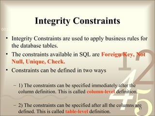
4210011 0010 1010 1101 0001 0100 1011
12
The CREATE TABLE
Command
Constraints in CREATE TABLEConstraints in CREATE TABLE

421
0011 0010 1010 1101 0001 0100 1011
13
CREATE TABLE Statement
• The CREATE TABLE Statement is used to create
tables to store data. Integrity Constraints like
primary key, unique key, foreign key can be
defined for the columns while creating the table.
The integrity constraints can be defined at column
level or table level. The implementation and the
syntax of the CREATE Statements differs for
different RDBMS.

421
0011 0010 1010 1101 0001 0100 1011
14
The Syntax for the CREATE
TABLE Statement
• CREATE TABLE table_name
(column_name1 datatype,
column_name2 datatype,
... column_nameN datatype
);
– table_name - is the name of the table.
– column_name1, column_name2.... - is the
name of the columns
– datatype - is the datatype for the column like
char, date, number etc.

421
0011 0010 1010 1101 0001 0100 1011
15
• For Example: If you want to create the
employee table, the statement would be
like,
CREATE TABLE employee
( id number(5),
name char(20),
dept char(10),
age number(2),
salary number(10),
location char(10)
);

421
0011 0010 1010 1101 0001 0100 1011
16
• Oracle provides another way of creating a
table.
• CREATE TABLE temp_employee
AS SELECT * FROM employee
• In the above statement, temp_employee
table is created with the same number of
columns and datatype as employee table.

421
0011 0010 1010 1101 0001 0100 1011
17
Integrity Constraints
• Integrity Constraints are used to apply business rules for
the database tables.
• The constraints available in SQL are Foreign Key, Not
Null, Unique, Check.
• Constraints can be defined in two ways
– 1) The constraints can be specified immediately after the
column definition. This is called column-level definition.
– 2) The constraints can be specified after all the columns are
defined. This is called table-level definition.

421
0011 0010 1010 1101 0001 0100 1011
18
1) Primary key:
• This constraint defines a column or combination of
columns which uniquely identifies each row in the
table.
• Syntax to define a Primary key at table level:
– [CONSTRAINT constraint_name] PRIMARY KEY
(column_name1,column_name2,..)
• Syntax to define a Primary key at column level:
– column name datatype [CONSTRAINT
constraint_name] PRIMARY KEY

421
0011 0010 1010 1101 0001 0100 1011
19
Primary Key at column level:
• CREATE TABLE employee
( id number(5) PRIMARY KEY,
name char(20),
dept char(10),
age number(2),
salary number(10),
location char(10)
); or
( id number(5) CONSTRAINT emp_id_pk PRIMARY KEY,
name char(20),
dept char(10),
age number(2),
salary number(10),
location char(10)
);

421
0011 0010 1010 1101 0001 0100 1011
20
Primary Key at table level:
( id number(5),
name char(20),
dept char(10),
age number(2),
salary number(10),
location char(10),
CONSTRAINT emp_id_pk PRIMARY KEY (id)
);

421
0011 0010 1010 1101 0001 0100 1011
21
2) Foreign key or Referential
Integrity :
• This constraint identifies any column referencing the
PRIMARY KEY in another table.
• It establishes a relationship between two columns in the
same table or between different tables.
• For a column to be defined as a Foreign Key, it should
be a defined as a Primary Key in the table which it is
referring.
• One or more columns can be defined as Foreign key.

421
0011 0010 1010 1101 0001 0100 1011
22
• Syntax to define a Foreign key at column
level:
– [CONSTRAINT constraint_name]
REFERENCES
Referenced_Table_name(column_name)
• Syntax to define a Foreign key at table level:
FOREIGN KEY(column_name)
REFERENCES
referenced_table_name(column_name);

421
0011 0010 1010 1101 0001 0100 1011
23
Foreign Key at column level:
• CREATE TABLE product
( product_id number(5) CONSTRAINT pd_id_pk PRIMARY KEY,
product_name char(20),
supplier_name char(20),
unit_price number(10)
);
• CREATE TABLE order_items
( order_id number(5) CONSTRAINT od_id_pk PRIMARY KEY,
product_id number(5) CONSTRAINT pd_id_fk REFERENCES
product(product_id),
);

421
0011 0010 1010 1101 0001 0100 1011
24
Foreign Key at table level:
• CREATE TABLE order_items
( order_id number(5) ,
product_id number(5),
CONSTRAINT od_id_pk PRIMARY
KEY(order_id),
CONSTRAINT pd_id_fk FOREIGN
KEY(product_id) REFERENCES
product(product_id)
);

421
0011 0010 1010 1101 0001 0100 1011
25
Foreign key in same table:
• If the employee table has a 'mgr_id' i.e, manager id as a
foreign key which references primary key 'id' within the
same table, the query would be like,
name char(20),
dept char(10),
age number(2),
mgr_id number(5) REFERENCES employee(id),
salary number(10),
location char(10)
);

421
0011 0010 1010 1101 0001 0100 1011
26
3) Not Null Constraint :
• This constraint ensures all rows in the table
contain a definite value for the column
which is specified as not null. Which means
a null value is not allowed.
• Syntax to define a Not Null constraint:
– [CONSTRAINT constraint name] NOT NULL

421
0011 0010 1010 1101 0001 0100 1011
27
• For Example: To create a employee table with Null
value, the query would be like
( id number(5),
name char(20) CONSTRAINT nm_nn NOT NULL,
dept char(10),
age number(2),
salary number(10),
location char(10)
);

421
0011 0010 1010 1101 0001 0100 1011
28
4) Unique Key:
• This constraint ensures that a column or a group
of columns in each row have a distinct value. A
column(s) can have a null value but the values
cannot be duplicated.
• Syntax to define a Unique key at column level:
– [CONSTRAINT constraint_name] UNIQUE
• Syntax to define a Unique key at table level:
UNIQUE(column_name)

421
0011 0010 1010 1101 0001 0100 1011
29
Unique Key at column level:
name char(20),
dept char(10),
age number(2),
salary number(10),
location char(10) UNIQUE
);
or
name char(20),
dept char(10),
age number(2),
salary number(10),
location char(10) CONSTRAINT loc_un UNIQUE
);

421
0011 0010 1010 1101 0001 0100 1011
30
Unique Key at table level:
name char(20),
dept char(10),
age number(2),
salary number(10),
location char(10),
CONSTRAINT loc_un UNIQUE(location)
);

421
0011 0010 1010 1101 0001 0100 1011
31
5) Check Constraint:
• This constraint defines a business rule on a column.
All the rows must satisfy this rule. The constraint
can be applied for a single column or a group of
columns.
• Syntax to define a Check constraint:
– [CONSTRAINT constraint_name] CHECK (condition)

421
0011 0010 1010 1101 0001 0100 1011
32
Check Constraint at column level:
name char(20),
dept char(10),
age number(2),
gender char(1) CHECK (gender in ('M','F')),
salary number(10),
location char(10)
);

421
0011 0010 1010 1101 0001 0100 1011
33
Check Constraint at table level:
name char(20),
dept char(10),
age number(2),
gender char(1),
salary number(10),
location char(10),
CONSTRAINT gender_ck CHECK (gender in ('M','F'))
);

421
0011 0010 1010 1101 0001 0100 1011
34
INSERT Statement
• The INSERT Statement is used to add new
rows of data to a table.
• We can insert data to a table in two ways
– Insert data directly to a table
– Insert data to a table through a select
statement

421
0011 0010 1010 1101 0001 0100 1011
35
1) Inserting the data directly to a
table
• Syntax for SQL INSERT is:
– INSERT INTO TABLE_NAME
[ (col1, col2, col3,...colN)]
VALUES (value1, value2, value3,...valueN);
or
– INSERT INTO TABLE_NAME
VALUES (value1, value2, value3,...valueN);

421
0011 0010 1010 1101 0001 0100 1011
36
• Example:
• INSERT INTO employee (id, name, dept, age,
salary) VALUES (105, 'Srinath', 'Aeronautics', 27,
33000);
• INSERT INTO employee
VALUES (105, 'Srinath', 'Aeronautics', 27, 33000);

421
0011 0010 1010 1101 0001 0100 1011
37
2) Inserting data to a table
through a select statement
• Syntax for SQL INSERT is:
• INSERT INTO table_name
[(column1, column2, ... columnN)]
SELECT column1, column2, ...columnN
FROM table_name [WHERE condition];

421
0011 0010 1010 1101 0001 0100 1011
38
• Example
• INSERT INTO employee (id, name, dept,
age, salary, location) SELECT emp_id,
emp_name, dept, age, salary, location
FROM temp_employee;

421
0011 0010 1010 1101 0001 0100 1011
39
SELECT Statement
• Use a SELECT statement or subquery to retrieve
data from one or more tables, object tables,
views, object views, or materialized views
• SELECT column_list FROM table-name
[WHERE Clause]
[GROUP BY clause]
[HAVING clause]
[ORDER BY clause];

421
0011 0010 1010 1101 0001 0100 1011
40
• For example to retrieve all rows from emp table
> select empno, ename, sal from emp; -- or
> select * from emp;
• Suppose you want to see only employee names
and their salaries then you can type the following
statement
> select name, sal from emp;
• If we want to display the first and last name of an
employee combined together, the SQL Select
Statement would be like
> SELECT first_name || ' ' || last_name FROM employee;

421
0011 0010 1010 1101 0001 0100 1011
41
Filtering Information using Where
Condition
• You can filter information using where
conditions like suppose you want to see
only those employees whose salary is above
5000 then you can type the following query
with where condition
> select * from emp where sal > 5000;

421
0011 0010 1010 1101 0001 0100 1011
42
Logical Conditions
• A logical condition combines the results of
two component conditions to produce a
single result based on them or to invert the
result of a single condition.

421
0011 0010 1010 1101 0001 0100 1011
43
Condition Operation Example
NOT Returns TRUE if the following
condition is FALSE.
ReturnsFALSE if it is TRUE.
If it is UNKNOWN, it
remains UNKNOWN.
SELECT *
FROM emp
WHERE NOT (sal IS NULL);
SELECT *
FROM emp
WHERE NOT
(salary BETWEEN 1000 AND 2000);
AND Returns TRUE if both
component conditions
are TRUE. Returns FALSE if
either is FALSE. Otherwise
returns UNKNOWN.
SELECT *
FROM employees
WHERE ename ='SAMI‘
AND sal=3000;
OR Returns TRUE if either
component condition
is TRUE. ReturnsFALSE if
both are FALSE. Otherwise
returns UNKNOWN.
SELECT *
FROM emp
WHERE ename = 'SAMI'
OR sal >= 1000;

421
0011 0010 1010 1101 0001 0100 1011
44
Membership Conditions
• A membership condition tests for membership in a
list or subquery
IN "Equal to any member of"
test. Equivalent to "= ANY".
SELECT * FROM emp
WHERE deptno IN (10,20);
SELECT * FROM emp
WHERE deptno IN (SELECT deptno
FROM dept WHERE city=’HYD’);
NOT IN Equivalent to "!=ALL".
Evaluates to FALSE if any
member of the set is NULL.
SELECT * FROM emp
WHERE ename NOT IN ('SCOTT',
'SMITH');

421
0011 0010 1010 1101 0001 0100 1011
45
Null Conditions
• A NULL condition tests for nulls.
• What is null?
– If a column is empty or no value has been inserted in it then
it is called null. Remember 0 is not null and blank string ‘ ’
is also not null.
IS [NOT]
NULL
Tests for nulls.
This is the only
condition that
you should use
to test for nulls.
SELECT ename
FROM emp
WHERE deptno
IS NULL;
SELECT * FROM emp WHERE ename IS NOT
NULL;

421
0011 0010 1010 1101 0001 0100 1011
46
EXISTS Condition
• An EXISTS condition tests for existence of rows in
a subquery.
EXISTS TRUE if a subquery returns
at least one row.
SELECT deptno
FROM dept d
WHERE EXISTS
(SELECT * FROM emp e
WHERE d.deptno = e.deptno);

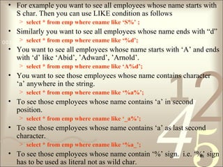
421
0011 0010 1010 1101 0001 0100 1011
47
LIKE Condition
• The LIKE conditions specify a test involving
pattern matching. Whereas the equality operator
(=) exactly matches one character value to
another, the LIKE conditions match a portion of
one character value to another by searching the
first value for the pattern specified by the
second. LIKE calculates strings using characters
as defined by the input character set.
• % for any number of characters
• _ for one character

421
0011 0010 1010 1101 0001 0100 1011
48
• For example you want to see all employees whose name starts with
S char. Then you can use LIKE condition as follows
> select * from emp where ename like ‘S%’ ;
• Similarly you want to see all employees whose name ends with “d”
> select * from emp where ename like ‘%d’;
• You want to see all employees whose name starts with ‘A’ and ends
with ‘d’ like ‘Abid’, ’Adward’, ’Arnold’.
> select * from emp where ename like ‘A%d’;
• You want to see those employees whose name contains character
‘a’ anywhere in the string.
> select * from emp where ename like ‘%a%’;
• To see those employees whose name contains ‘a’ in second
position.
> select * from emp where ename like ‘_a%’;
• To see those employees whose name contains ‘a’ as last second
character.
> select * from emp where ename like ‘%a_’;
• To see those employees whose name contain ‘%’ sign. i.e. ‘%’ sign
has to be used as literal not as wild char.

421
0011 0010 1010 1101 0001 0100 1011
49
ORDER BY
• The ORDER BY clause is used in a SELECT
statement to sort results either in ascending or
descending order. Oracle sorts query results in
ascending order by default.
• Syntax for using SQL ORDER BY clause to
sort data is:
– SELECT column-list
FROM table_name [WHERE condition]
[ORDER BY column1 [, column2, .. columnN]
[DESC]];

421
0011 0010 1010 1101 0001 0100 1011
50
• If you want to sort the employee table by salary of the
employee, the sql query would be.
> SELECT name, salary FROM employee ORDER BY salary;
• If you want to sort the employee table by the name and
salary, the query would be like,
> SELECT name, salary FROM employee ORDER BY name,
salary;
• You can represent the columns in the ORDER BY clause
by specifying the position of a column in the SELECT
list, instead of writing the column name.
> SELECT name, salary FROM employee ORDER BY 1, 2;
• NOTE:The columns specified in ORDER BY clause
should be one of the columns selected in the SELECT
column list.

421
0011 0010 1010 1101 0001 0100 1011
51
• By default, the ORDER BY Clause sorts data in
ascending order. If you want to sort the data in
descending order, you must explicitly specify it as
shown below.
> SELECT name, salary
FROM employee
ORDER BY name, salary DESC;
– The above query sorts only the column 'salary' in descending
order and the column 'name' by ascending order.
• If you want to select both name and salary in
descending order, the query would be as given below.
> SELECT name, salary
FROM employee
ORDER BY name DESC, salary DESC;

421
0011 0010 1010 1101 0001 0100 1011
52
• If you want to display employee name, current salary,
and a 20% increase in the salary for only those
employees for whom the percentage increase in salary is
greater than 30000 and in descending order of the
increased price, the SELECT statement can be written as
shown below
> SELECT name, salary, salary*1.2 AS new_salary
FROM employee
WHERE salary*1.2 > 30000
ORDER BY new_salary DESC;
• NOTE:Aliases defined in the SELECT Statement can be
used in ORDER BY Clause.

421
0011 0010 1010 1101 0001 0100 1011
53
GROUP BY Clause
• The SQL GROUP BY Clause is used along with
the group functions to retrieve data grouped
according to one or more columns.
• If you want to know the total amount of salary
spent on each department, the query would be:
> SELECT dept, SUM (salary)
FROM employee
GROUP BY dept;

421
0011 0010 1010 1101 0001 0100 1011
54
• NOTE: The group by clause should contain
all the columns in the select list expect
those used along with the group functions.
> SELECT location, dept, SUM (salary)
FROM employee
GROUP BY location, dept;

421
0011 0010 1010 1101 0001 0100 1011
55
HAVING Clause
• Having clause is used to filter data based on
the group functions. This is similar to
WHERE condition but is used with group
functions.

421
0011 0010 1010 1101 0001 0100 1011
56
• If you want to select the department that has total salary
paid for its employees more than 25000, the sql query
would be like;
> SELECT dept, SUM (salary)
FROM employee
GROUP BY dept
HAVING SUM (salary) > 25000
• When WHERE, GROUP BY and HAVING clauses are
used together in a SELECT statement, the WHERE
clause is processed first, then the rows that are returned
after the WHERE clause is executed are grouped based
on the GROUP BY clause. Finally, any conditions on
the group functions in the HAVING clause are applied
to the grouped rows before the final output is displayed.

421
0011 0010 1010 1101 0001 0100 1011
57
Delete Statement
• The DELETE Statement is used to delete rows from a
table.
The Syntax of a SQL DELETE statement is:
DELETE FROM table_name [WHERE condition];
table_name -- the table name which has to be updated.
• NOTE:The WHERE clause in the sql delete command is
optional and it identifies the rows in the column that gets
deleted. If you do not include the WHERE clause all the
rows in the table is deleted, so be careful while writing a
DELETE query without WHERE clause.

421
0011 0010 1010 1101 0001 0100 1011
58
• For Example: To delete an employee with id 100
from the employee table, the sql delete query would
be like,
DELETE FROM employee WHERE id = 100;
• To delete all the rows from the employee table, the
query would be like,
DELETE FROM employee;

421
0011 0010 1010 1101 0001 0100 1011
59
TRUNCATE Statement
• The SQL TRUNCATE command is used to delete
all the rows from the table and free the space
containing the table.
Syntax to TRUNCATE a table:
TRUNCATE TABLE table_name;
• For Example: To delete all the rows from
employee table, the query would be like,
TRUNCATE TABLE employee;

421
0011 0010 1010 1101 0001 0100 1011
60
DROP Statement
• The SQL DROP command is used to remove an
object from the database. If you drop a table, all the
rows in the table is deleted and the table structure is
removed from the database. Once a table is dropped
we cannot get it back, so be careful while using
DROP command. When a table is dropped all the
references to the table will not be valid.

421
0011 0010 1010 1101 0001 0100 1011
61
• Syntax to drop a sql table structure:
DROP TABLE table_name;
• For Example: To drop the table employee,
the query would be like
DROP TABLE employee;

421
0011 0010 1010 1101 0001 0100 1011
62
DROP, DELETE, & TRUNCATE
• DROP:
– Relationship with other table will be invalid.
– Integrity constraint will be dropped.
– Access privileges will be dropped.
• DELETE:
– Only deletes the rows.
– It does not free the space contained by the table.
• TRUNCATE:
– Deletes all the rows.
– Frees the space contained by the table.

421
0011 0010 1010 1101 0001 0100 1011
63
UPDATE Statement
• The UPDATE Statement is used to modify the existing rows
in a table.
The Syntax for SQL UPDATE Command is:
UPDATE table_name
SET column_name1 = value1,
column_name2 = value2, ...
[WHERE condition];
– table_name - the table name which has to be updated.
– column_name1, column_name2.. - the columns that gets changed.
– value1, value2... - are the new values.
• NOTE: In the Update statement, WHERE clause identifies
the rows that get affected. If you do not include the
WHERE clause, column values for all the rows get affected.

421
0011 0010 1010 1101 0001 0100 1011
64
• For Example: To update the location of an
employee, the sql update query would be like,
UPDATE employee
SET location ='Mysore'
WHERE id = 101;
• To change the salaries of all the employees, the
query would be,
UPDATE employee
SET salary = salary + (salary * 0.2);

421
0011 0010 1010 1101 0001 0100 1011
65
ALTER TABLE Statement
• The SQL ALTER TABLE command is used to
modify the definition (structure) of a table by
modifying the definition of its columns. The
ALTER command is used to perform the following
functions.
1) Add, drop, modify table columns
2) Add and drop constraints
3) Enable and Disable constraints

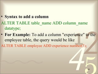
421
0011 0010 1010 1101 0001 0100 1011
66
• Syntax to add a column
ALTER TABLE table_name ADD column_name
datatype;
• For Example: To add a column "experience" to the
employee table, the query would be like
ALTER TABLE employee ADD experience number(3);

421
0011 0010 1010 1101 0001 0100 1011
67
• Syntax to drop a column
ALTER TABLE table_name DROP column_name;
• For Example: To drop the column "location" from
the employee table, the query would be like
ALTER TABLE employee DROP column location;

421
0011 0010 1010 1101 0001 0100 1011
68
• Syntax to modify a column
ALTER TABLE table_name MODIFY column_name
datatype;
• For Example: To modify the column salary in the
employee table, the query would be like
ALTER TABLE employee MODIFY salary number(15,2);

421
0011 0010 1010 1101 0001 0100 1011
Using an ALTER TABLE
statement
• The syntax for creating a primary key in an
ALTER TABLE statement is:
• ALTER TABLE table_name add
CONSTRAINT constraint_name PRIMARY
KEY (column1, column2, ... column_n);
For Example
• ALTER TABLE supplier add CONSTRAINT
supplier_pk PRIMARY KEY (supplier_id);
69

421
0011 0010 1010 1101 0001 0100 1011
Drop a Primary Key
• The syntax for dropping a primary key is:
• ALTER TABLE table_name drop
CONSTRAINT constraint_name;
For Example
• ALTER TABLE supplier drop
CONSTRAINT supplier_pk;
70

421
0011 0010 1010 1101 0001 0100 1011
Alter- Foreign Key
create table tab1
(d_id number primary key,
d_name varchar2(20)
)
71

421
0011 0010 1010 1101 0001 0100 1011
create table tab2
(
e_id number primary key,
e_name varchar2(20),
e_dept number
)
72

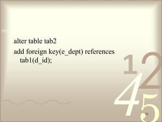
421
0011 0010 1010 1101 0001 0100 1011
alter table tab2
add foreign key(e_dept) references
tab1(d_id);
73

421
0011 0010 1010 1101 0001 0100 1011
74
RENAME Command
• The SQL RENAME command is used to change the name
of the table or a database object.
• If you change the object's name any reference to the old
name will be affected. You have to manually change the old
name to the new name in every reference.
• Syntax to rename a table
RENAME old_table_name To new_table_name;
• For Example: To change the name of the table employee to
my_employee, the query would be like
RENAME employee TO my_emloyee;

Oracle sql ppt1

More Related Content

What's hot (20)

Similar to Oracle sql ppt1 (20)

More from Madhavendra Dutt (12)

Recently uploaded (20)

Oracle sql ppt1

Editor's Notes