


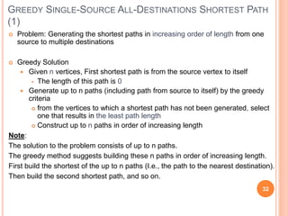
![GREEDY ATTEMPTS FOR 0/1 KNAPSACK
Apply greedy method:
Greedy attempt on capacity utilization
Greedy criterion: select items in increasing order of weight
When n = 2, c = 7, w = [3, 6], p = [2, 10],
if only item 1 is selected profit of selection is 2 not best
selection!
Greedy attempt on profit earned
Greedy criterion: select items in decreasing order of profit
When n = 3, c = 7, w = [7, 3, 2], p = [10, 8, 6],
if only item 1 is selected profit of selection is 10 not best
selection!
28](https://image.slidesharecdn.com/parallelalgorithmsincombinatorialoptimizationproblems-230318100707-326d0849/85/Parallel_Algorithms_In_Combinatorial_Optimization_Problems-ppt-28-320.jpg)

![GREEDY SINGLE SOURCE ALL DESTINATIONS: EXAMPLE (1)
1
2
3
4
5
6
7
2
6
16
7
8
10
3
14
4
4
5 3
1
[1] [2] [3] [4] [5] [6] [7]
d
p
0
-
1
2
3
4 7
6
1
2
1
16
1
-
-
-
-
14
1
2
34](https://image.slidesharecdn.com/parallelalgorithmsincombinatorialoptimizationproblems-230318100707-326d0849/85/Parallel_Algorithms_In_Combinatorial_Optimization_Problems-ppt-34-320.jpg)
![GREEDY SINGLE SOURCE ALL DESTINATIONS : EXAMPLE
(2)
1
2
3
4
5
6
7
2
6
16
7
8
10
3
14
4
4
5 3
1
[1] [2] [3] [4] [5] [6] [7]
d
p
1
0
-
6
1
2
1
16
1
-
-
-
-
14
1
1 3
2
5
6
5
3
10
3
5
35](https://image.slidesharecdn.com/parallelalgorithmsincombinatorialoptimizationproblems-230318100707-326d0849/85/Parallel_Algorithms_In_Combinatorial_Optimization_Problems-ppt-35-320.jpg)
![GREEDY SINGLE SOURCE ALL DESTINATIONS : EXAMPLE
(3)
1
2
3
4
5
6
7
2
6
16
7
8
10
3
14
4
4
5 3
1
[1] [2] [3] [4] [5] [6] [7]
d
p
1
0
-
6
1
2
1
16
1
-
-
-
-
14
1
1 3
5
3
10
3
1 3 5
4 7
9
5
6
36](https://image.slidesharecdn.com/parallelalgorithmsincombinatorialoptimizationproblems-230318100707-326d0849/85/Parallel_Algorithms_In_Combinatorial_Optimization_Problems-ppt-36-320.jpg)
![GREEDY SINGLE SOURCE ALL DESTINATIONS : EXAMPLE
(4)
1
2
3
4
5
6
7
2
6
16
7
8
10
3
14
4
4
5 3
1
[1] [2] [3] [4] [5] [6] [7]
d
p
1
0
-
6
1
2
1
9
5
-
-
-
-
14
1
1 3
5
3
10
3
1 3 5
1 2
4
9
37](https://image.slidesharecdn.com/parallelalgorithmsincombinatorialoptimizationproblems-230318100707-326d0849/85/Parallel_Algorithms_In_Combinatorial_Optimization_Problems-ppt-37-320.jpg)
![GREEDY SINGLE SOURCE ALL DESTINATIONS : EXAMPLE
(5)
1
2
3
4
5
6
7
2
6
16
7
8
10
3
14
4
4
5 3
1
[1] [2] [3] [4] [5] [6] [7]
d
p
1
0
-
6
1
2
1
9
5
-
-
-
-
14
1
1 3
5
3 3
1 3 5
1 2
1 3 5 4
7
12
4
1
0
38](https://image.slidesharecdn.com/parallelalgorithmsincombinatorialoptimizationproblems-230318100707-326d0849/85/Parallel_Algorithms_In_Combinatorial_Optimization_Problems-ppt-38-320.jpg)
![GREEDY SINGLE SOURCE ALL DESTINATIONS : EXAMPLE
(6)
1
2
3
4
5
6
7
2
6
16
7
8
10
3
14
4
4
5 3
1
[1] [2] [3] [4] [5] [6] [7]
d
p
0
-
6
1
2
1
9
5
-
-
-
-
14
1
5
3
10
3
12
4
1 3 6
7
11
6
39](https://image.slidesharecdn.com/parallelalgorithmsincombinatorialoptimizationproblems-230318100707-326d0849/85/Parallel_Algorithms_In_Combinatorial_Optimization_Problems-ppt-39-320.jpg)

Parallel_Algorithms_In_Combinatorial_Optimization_Problems.ppt
- 1. CS 6260 PARALLEL COMPUTATION PARALLEL ALGORITHMS IN COMBINATORIAL OPTIMIZATION PROBLEMS Professor: Elise De Doncker Presented By: Lina Hussein 1
- 2. TOPICS COVERED ARE: Backtracking Branch and bound Divide and conquer Greedy Methods Short paths algorithms 2
- 3. BRANCH AND BOUND Branch and bound (BB) is a general algorithm for finding optimal solutions of various optimization problems, especially in discrete and combinatorial optimization. It consists of a systematic enumeration of all candidate solutions, where large subsets of fruitless candidates are discarded en masse (all together), by using upper and lower estimated bounds of the quantity being optimized. 3
- 4. BRANCH AND BOUND If we picture the subproblems graphically, then we form a search tree. Each subproblem is linked to its parent and eventually to its children. Eliminating a problem from further consideration is called pruning or fathoming. The act of bounding and then branching is called processing. A subproblem that has not yet been considered is called a candidate for processing. The set of candidates for processing is called the candidate list. Going back on the path from a node to its root is called backtracking. 4
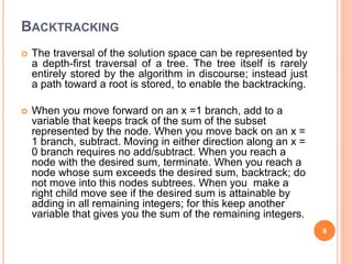
- 5. BACKTRACKING Backtracking is a general algorithm for finding all (or some) solutions to some computational problem, that incrementally builds candidates to the solutions, and abandons each partial candidate ("backtracks") as soon as it determines that it cannot possibly be completed to a valid solution.. The Algorithm systematically searches for a solution to a problem among all available options. It does so by assuming that the solutions are represented by vectors (v1, ..., vi) of values and by traversing in a depth first manner the domains of the vectors until the solutions are found. 5
- 6. BACKTRACKING A systematic way to iterate through all the possible configurations of a search space. Solution: a vector v = (v1,v2,…,vi) At each step, we start from a given partial solution, say, v=(v1,v2,…,vk), and try to extend it by adding another element at the end. If so, we should count (or print,…) it. If not, check whether possible extension exits. If so, recur and continue If not, delete vk and try another possibility. ALGORITHM try(v1,...,vi) IF (v1,...,vi) is a solution THEN RETURN (v1,...,vi) FOR each v DO IF (v1,...,vi,v) is acceptable vector THEN sol = try(v1,...,vi,v) IF sol != () THEN RETURN sol END END RETURN () 6
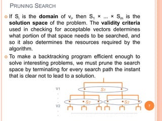
- 7. PRUNING SEARCH If Si is the domain of vi, then S1 × ... × Sm is the solution space of the problem. The validity criteria used in checking for acceptable vectors determines what portion of that space needs to be searched, and so it also determines the resources required by the algorithm. To make a backtracking program efficient enough to solve interesting problems, we must prune the search space by terminating for every search path the instant that is clear not to lead to a solution. 7 S1 S2 S2 V1 . . . V2 . . ...........................................................
- 8. BACKTRACKING The traversal of the solution space can be represented by a depth-first traversal of a tree. The tree itself is rarely entirely stored by the algorithm in discourse; instead just a path toward a root is stored, to enable the backtracking. When you move forward on an x =1 branch, add to a variable that keeps track of the sum of the subset represented by the node. When you move back on an x = 1 branch, subtract. Moving in either direction along an x = 0 branch requires no add/subtract. When you reach a node with the desired sum, terminate. When you reach a node whose sum exceeds the desired sum, backtrack; do not move into this nodes subtrees. When you make a right child move see if the desired sum is attainable by adding in all remaining integers; for this keep another variable that gives you the sum of the remaining integers. 8
- 9. BACKTRACKING DEPTH-FIRST SEARCH x1=1 x1= 0 x2=1 x2= 0 x2=1 x2= 0 9
- 10. BACKTRACKING DEPTH-FIRST SEARCH x1=1 x1= 0 x2=1 x2= 0 x2=1 x2= 0 10
- 11. BACKTRACKING DEPTH-FIRST SEARCH x1=1 x1= 0 x2=1 x2= 0 x2=1 x2= 0 11
- 12. BACKTRACKING DEPTH-FIRST SEARCH x1=1 x1= 0 x2=1 x2= 0 x2=1 x2= 0 12
- 13. BACKTRACKING DEPTH-FIRST SEARCH x1=1 x1= 0 x2=1 x2= 0 x2=1 x2= 0 13
- 14. BACKTRACKING DEPTH-FIRST SEARCH x1=1 x1= 0 x2=1 x2= 0 x2=1 x2= 0 14
- 15. EXAMPLE Example of the use Branch and Bound & backtracking is Puzzles! For such problems, solutions are at different levels of the tree http://www.hbmeyer.de/backtrack/backtren.htm 15 1 2 3 4 5 6 7 8 9 1011 12 131415 1 3 2 4 5 6 13 14 15 12 11 10 9 7 8
- 16. TOPICS COVERED ARE: Branch and bound Backtracking Divide and conquer Greedy Methods Short paths algorithms 16
- 17. DIVIDE AND CONQUER divide and conquer (D&C) is an important algorithm design paradigm based on multi-branched recursion. The algorithm works by recursively breaking down a problem into two or more sub-problems of the same (or related) type, until these become simple enough to be solved directly. The solutions to the sub-problems are then combined to give a solution to the original problem. This technique is the basis of efficient algorithms for all kinds of problems, such as sorting (e.g., quick sort, merge sort). 17
- 18. ADVANTAGES Solving difficult problems: Divide and conquer is a powerful tool for solving conceptually difficult problems, such as the classic Tower of Hanoi puzzle: it break the problem into sub-problems, then solve the trivial cases and combine sub-problems to the original problem. Roundoff control In computations with rounded arithmetic, e.g. with floating point numbers, a D&C algorithm may yield more accurate results than any equivalent iterative method. Example, one can add N numbers either by a simple loop that adds each datum to a single variable, or by a D&C algorithm that breaks the data set into two halves, recursively computes the sum of each half, and then adds the two sums. While the second method performs the same number of additions as the first, and pays the overhead of the recursive calls, it is usually more accurate. 18
- 19. IN PARALLELISM... Divide and conquer algorithms are naturally adapted for execution in multi-processor machines, especially shared-memory systems where the communication of data between processors does not need to be planned in advance, because distinct sub-problems can be executed on different processors. 19
- 20. TOPICS COVERED ARE: Branch and bound Backtracking Divide and conquer Greedy Methods Short paths algorithms 20
- 21. GREEDY METHODS A greedy algorithm: is any algorithm that follows the problem solving metaheuristic of making the locally optimal choice at each stage with the hope of finding the global optimum. A metaheuristic method: Is method for solving a very general class of computational problems that aims on obtaining a more efficient or more robust procedure for the problem. Generally it is applied to problems for which there is no satisfactory problem-specific algorithm designed to solve it. It targeted to the combinatorial optimization (problems that’s are a problems in which has an optimization function to( minimize or maximize) subject to some constraints and its goal is to find the best possible solution 21
- 22. EXAMPLES The vehicle routing problem (VRP) A number of goods need to be moved from certain pickup locations to other delivery locations. The goal is to find optimal routes for a fleet of vehicles to visit the pickup and drop-off locations. Travelling salesman problem Given a list of cities and their pair wise distances, the task is to find a shortest possible tour that visits each city exactly once. Coin Change (making change for n $ using minimum number of coins) The knapsack problem The Shortest Path Problem 22
- 23. KNAPSACK The knapsack problem or rucksack problem is a problem in combinatorial optimization. It derives its name from the following maximization problem of the best choice of essentials that can fit into one bag to be carried on a trip. Given a set of items, each with a weight and a value, determine the number of each item to include in a collection so that the total weight is less than a given limit and the total value is as large as possible. 23
- 24. THE ORIGINAL KNAPSACK PROBLEM (1) Problem Definition Want to carry essential items in one bag Given a set of items, each has A cost (i.e., 12kg) A value (i.e., 4$) Goal To determine the # of each item to include in a collection so that The total cost is less than some given cost And the total value is as large as possible 24
- 25. THE ORIGINAL KNAPSACK PROBLEM (2) Three Types 0/1 Knapsack Problem restricts the number of each kind of item to zero or one Bounded Knapsack Problem restricts the number of each item to a specific value Unbounded Knapsack Problem places no bounds on the number of each item Complexity Analysis The general knapsack problem is known to be NP-hard No polynomial-time algorithm is known for this problem Here, we use greedy heuristics which cannot guarantee the optimal solution 25
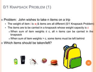
- 26. 0/1 KNAPSACK PROBLEM (1) Problem: John wishes to take n items on a trip The weight of item i is wi & items are all different (0/1 Knapsack Problem) The items are to be carried in a knapsack whose weight capacity is c When sum of item weights ≤ c, all n items can be carried in the knapsack When sum of item weights > c, some items must be left behind Which items should be taken/left? 26
- 27. 0/1 KNAPSACK PROBLEM (2) John assigns a profit pi to item i All weights and profits are positive numbers John wants to select a subset of the n items to take The weight of the subset should not exceed the capacity of the knapsack (constraint) Cannot select a fraction of an item (constraint) The profit of the subset is the sum of the profits of the selected items (optimization function) The profit of the selected subset should be maximum (optimization criterion) Let xi = 1 when item i is selected and xi = 0 when item i is not selected Because this is a 0/1 Knapsack Problem, you can choose the item or not choose it. 27
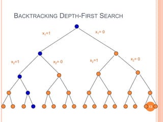
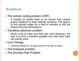
- 28. GREEDY ATTEMPTS FOR 0/1 KNAPSACK Apply greedy method: Greedy attempt on capacity utilization Greedy criterion: select items in increasing order of weight When n = 2, c = 7, w = [3, 6], p = [2, 10], if only item 1 is selected profit of selection is 2 not best selection! Greedy attempt on profit earned Greedy criterion: select items in decreasing order of profit When n = 3, c = 7, w = [7, 3, 2], p = [10, 8, 6], if only item 1 is selected profit of selection is 10 not best selection! 28
- 29. THE SHORTEST PATH PROBLEM Path length is sum of weights of edges on path in directed weighted graph The vertex at which the path begins is the source vertex The vertex at which the path ends is the destination vertex Goal To find a path between two vertices such that the sum of the weights of its edges is minimized 29
- 30. TYPES OF THE SHORTEST PATH PROBLEM Three types Single-source single-destination shortest path Single-source all-destinations shortest path All pairs (every vertex is a source and destination) shortest path 30
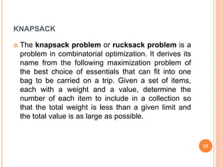
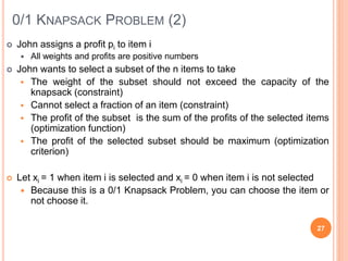
- 31. SINGLE-SOURCE SINGLE-DESTINATION SHORTED PATH Possible greedy algorithm Leave the source vertex using the cheapest edge Leave the current vertex using the cheapest edge to the next vertex Continue until destination is reached Try Shortest 1 to 7 Path by this Greedy Algorithm the algorithm does not guarantee the optimal solution 31 1 2 3 4 5 6 7 2 6 16 7 8 10 3 14 4 4 5 3 1
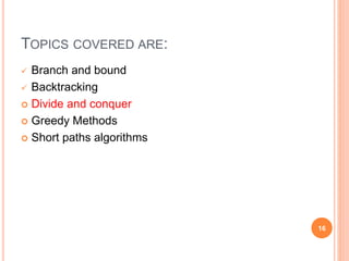
- 32. GREEDY SINGLE-SOURCE ALL-DESTINATIONS SHORTEST PATH (1) Problem: Generating the shortest paths in increasing order of length from one source to multiple destinations Greedy Solution Given n vertices, First shortest path is from the source vertex to itself The length of this path is 0 Generate up to n paths (including path from source to itself) by the greedy criteria from the vertices to which a shortest path has not been generated, select one that results in the least path length Construct up to n paths in order of increasing length Note: The solution to the problem consists of up to n paths. The greedy method suggests building these n paths in order of increasing length. First build the shortest of the up to n paths (I.e., the path to the nearest destination). Then build the second shortest path, and so on. 32
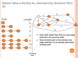
- 33. GREEDY SINGLE-SOURCE ALL-DESTINATIONS SHORTEST PATH (2) 33 1 2 3 4 5 6 7 2 6 16 7 8 10 3 14 4 4 5 3 1 Path Length 1 0 1 3 2 1 3 5 5 1 2 6 1 3 9 5 4 1 3 10 6 1 3 11 6 7 Each path (other than first) is a one edge extension of a previous path Next shortest path is the shortest one edge extension of an already generated shortest path Increasing order
- 34. GREEDY SINGLE SOURCE ALL DESTINATIONS: EXAMPLE (1) 1 2 3 4 5 6 7 2 6 16 7 8 10 3 14 4 4 5 3 1 [1] [2] [3] [4] [5] [6] [7] d p 0 - 1 2 3 4 7 6 1 2 1 16 1 - - - - 14 1 2 34
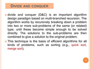
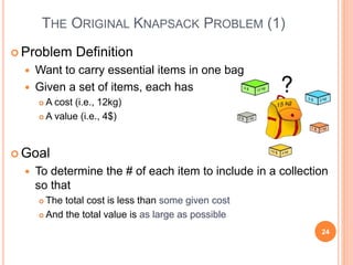
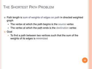
- 35. GREEDY SINGLE SOURCE ALL DESTINATIONS : EXAMPLE (2) 1 2 3 4 5 6 7 2 6 16 7 8 10 3 14 4 4 5 3 1 [1] [2] [3] [4] [5] [6] [7] d p 1 0 - 6 1 2 1 16 1 - - - - 14 1 1 3 2 5 6 5 3 10 3 5 35
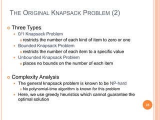
- 36. GREEDY SINGLE SOURCE ALL DESTINATIONS : EXAMPLE (3) 1 2 3 4 5 6 7 2 6 16 7 8 10 3 14 4 4 5 3 1 [1] [2] [3] [4] [5] [6] [7] d p 1 0 - 6 1 2 1 16 1 - - - - 14 1 1 3 5 3 10 3 1 3 5 4 7 9 5 6 36
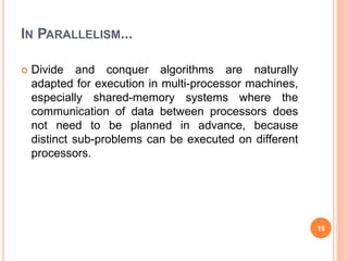
- 37. GREEDY SINGLE SOURCE ALL DESTINATIONS : EXAMPLE (4) 1 2 3 4 5 6 7 2 6 16 7 8 10 3 14 4 4 5 3 1 [1] [2] [3] [4] [5] [6] [7] d p 1 0 - 6 1 2 1 9 5 - - - - 14 1 1 3 5 3 10 3 1 3 5 1 2 4 9 37
- 38. GREEDY SINGLE SOURCE ALL DESTINATIONS : EXAMPLE (5) 1 2 3 4 5 6 7 2 6 16 7 8 10 3 14 4 4 5 3 1 [1] [2] [3] [4] [5] [6] [7] d p 1 0 - 6 1 2 1 9 5 - - - - 14 1 1 3 5 3 3 1 3 5 1 2 1 3 5 4 7 12 4 1 0 38
- 39. GREEDY SINGLE SOURCE ALL DESTINATIONS : EXAMPLE (6) 1 2 3 4 5 6 7 2 6 16 7 8 10 3 14 4 4 5 3 1 [1] [2] [3] [4] [5] [6] [7] d p 0 - 6 1 2 1 9 5 - - - - 14 1 5 3 10 3 12 4 1 3 6 7 11 6 39
- 40. TOPICS COVERED ARE: Backtracking Branch and bound Divide and conquer Greedy Methods Short path algorithm 40
- 41. Parallel Algorithms Arrays and Trees Packet Routing Greedy Algorithms Knapsack Problem Graph Algorithms Short paths Meshes of Trees Hypercube…& Networks Combinatorial optimization problems 41 .. A branch of optimization. Its domain is optimization problems where the set of feasible solutions is discrete or can be reduced to a discrete one, and the goal is to find the best possible solution
- 42. USE OF ALGORITHMS IN PARALLEL With Parallelism many Problems appeared , some are those of choice of granularity such as Grouping of tasks or partitioning, scheduling.. And when the physical architecture is to be taken into account we face the Mapping problem. Greedy Methods Packet routing Routes every packets to its destination through the shortest path. Shortest path Graph algorithms To compute the least weight directed path between any two nodes in a weighted graph. 42
- 43. Branch and Bound Exact Methods ..Based on exploring all possible solutions. In theory it gives optimal solutions but in practice it can be costly an unusable for large problems. It uses B&B in Mapping Problem: A mapping, is an application allocation which associate a processor with a task. The B&B algorithms will involve mapping a task progressively between processors by scanning a search tree that gives all possible combinations. For each mapping a partial solution is given and for each one a set of less restricted partial solutions is constructed similarly by mapping a second task and so on until all the tasks have been mapped(leaves of the tree are reached). For each node the cost of mapping is computed then all branches can be pruned through an estimating function and he best computed mapping is then choosed. 43 USE OF ALGORITHMS IN PARALLEL
- 44. Q & A BRANCH AND BOUND VS. BACKTRACKING? B&B is An enhancement of backtracking Similarity A state space tree is used to solve a problem. Difference The branch-and-bound algorithm does not limit us to any particular way of traversing the tree and is used only for optimization problems The backtracking algorithm requires traversing the tree and is used for non-optimization problems as well. 44
- 45. REFERENCES Parallel Algorithms and Architectures ,by Michel Cosnard, Denis Trystram. Parallel and sequential algorithms.. Greedy Method and Compression, Goodrich Tamassia http://www.wikipedia.org/ 45