PHYSICS 2 ELECTRICITY MAGNETISM OPTICS AND MODERN PHYSICS.pdf

PHYSICS 1: MECHANICS AND THERMODYNAMICS
PHYSICS 2: ELECTRICITY, MAGNETISM, OPTICS,
AND MODERN PHYSICS

PART 4
Electricity and Magnetism
Chapter 1: Electric Fields
Chapter 2: Gauss’s Law
Chapter 3: Electric Potential
Chapter 4: Capacitance and Dielectrics
Chapter 5: Current and Resistance
Chapter 6: Direct-Current Circuits
Chapter 7: Magnetic Fields
Chapter 8: Sources of the Magnetic Field
Chapter 9: Faraday’s Law

CHAPTER 1 (3)
ELECTRIC FIELDS
1.1 Properties of Electric Charges
1.2 Charging Objects by Induction
1.3 Coulomb’s Law
1.4 Analysis Model: Particle in a
Field (Electric)
1.5 Electric Field of a Continuous
Charge Distribution
1.6 Electric Field Lines (study in
chapter 2)
1.7 Motion of a Charged Particle
in a Uniform Electric Field

Charge interaction:
Charge of the same
sign repel one
another.
Charges with
opposite signs
attract one another.
 Electric charge is
always conserved in
an isolated system.
CHAPTER 1 - ELECTRIC FIELDS
Two types of charges: positive and negative

Positive ion: 𝑞+ = 𝑁𝑒, Negative ion: 𝑞− = −𝑁𝑒
Electric charge always occurs as integral multiples of a
fundamental amount of charge 𝑒 (quantized):
𝑞 = ±𝑁𝑒
Neutron: 𝑞𝑛 = 0, Proton: 𝑞𝑝 = 𝑒, Electron: 𝑞𝑒 = −𝑒

Three objects are brought close to each other, two at a time.
When objects A and B are brought together, they repel. When
objects B and C are brought together, they also repel. Which of
the following are true?
(a) Objects A and C possess charges of the same sign.
(b) Objects A and C possess charges of opposite sign.
(c) All three objects possess charges of the same sign.
(d) One object is neutral.
(e) Additional experiments must be performed to determine the
signs of the charges.

Electrical conductors are materials in which some of the
electrons are free electrons that are not bound to atoms and
can move relatively freely through the material. Ex.: copper,
aluminum, silver,…
Electrical insulators are materials in which all electrons are
bound to atoms and cannot move freely through the
material. Ex.: glass, rubber, dry wood,…
Semiconductors are a third class of materials, and their
electrical properties are somewhere between those of
insulators and those of conductors. Ex.: Silicon,
germanium,…

Three objects are brought close to one another, two at a time.
When objects A and B are brought together, they attract. When
objects B and C are brought together, they repel. Which of the
following are necessarily true?
(a) Objects A and C possess charges of the same sign.
(b) Objects A and C possess charges of opposite sign.
(c) All three objects possess charges of the same sign.
(d) One object is neutral.
(e) Additional experiments must be performed to determine
information about the charges on the objects.

Electric force between two stationary point charges
(called electrostatic force or Coulomb force):
𝑭𝒆 = 𝒌𝒆
𝒒𝟏 𝒒𝟐
𝒓𝟐
 Coulomb constance:
𝑘𝑒 =
1
4𝜋𝜀0
= 8.987 × 109 N. m2/C2
where 𝜀0 is permittivity of free space
𝜀0 = 8.854 × 10−12 C2/m2N
 𝑞1 , 𝑞2 : magnitude of point charges
 𝑟: distance between two charges
 Point charge: charged particle of zero size
1.3 Coulomb’s Law

Example 1.1
The electron and proton of a hydrogen atom are separated (on the average)
by a distance of approximately 5.3 × 10-11 m. Find the magnitudes of the
electric force and the gravitational force between the two particles.
1.3 Coulomb’s Law

Vector form of Coulomb’s law:
The electric force exerted by a charge
𝒒𝟏 on a second charge 𝒒𝟐
𝑭𝟏𝟐 = 𝒌𝒆
𝒒𝟏𝒒𝟐
𝒓𝟐 𝒓𝟏𝟐
 𝒓𝟏𝟐 is a unit vector directed from 𝑞1
toward 𝑞2
 The force exerted by 𝑞2 on 𝑞1
𝐹21 = −𝐹12
 When more than two charges are
present, for example, if four charges
are present, the resultant force
exerted by particles 2, 3, and 4 on
particle 1 is
𝑭𝟏 = 𝑭𝟐𝟏 + 𝑭𝟑𝟏 + 𝑭𝟒𝟏
1.3 Coulomb’s Law

The Superposition Principle
1.3 Coulomb’s Law

1.3 Coulomb’s Law
Object A has a charge of +2 µC, and object B has a charge of
+6 µC. Which statement is true about the electric forces on
the objects?
(a) 𝐹𝐴𝐵 = −3𝐹𝐵𝐴
(b) 𝐹𝐴𝐵 = −𝐹𝐵𝐴
(c) 3𝐹𝐴𝐵 = −𝐹𝐵𝐴
(d) 𝐹𝐴𝐵 = 3𝐹𝐵𝐴
(e) 𝐹𝐴𝐵 = 𝐹𝐵𝐴
(f) 3𝐹𝐴𝐵 = 𝐹𝐵𝐴

Example 1.2
Consider three point
charges located at the
corners of a right triangle as
shown in the below figure,
where 𝑞1 = 𝑞3 = 5.00 μC ,
𝑞2 = −2.00 μC , and 𝑎 =
0.100 m. Find the resultant
force exerted on 𝑞3.
1.3 Coulomb’s Law

1.3 Coulomb’s Law
Example 1.2

EX1: Charge q1 = 25 nC is at
the origin, charge q2 = -15 nC
is on the axis at x = 2.0 m,
and charge q0 = 20 nC is at
the point x = 2 m, y = 2 m.
Find the magnitude and
direction of the resultant
electric force on q0.
1.3 Coulomb’s Law

EX2: Two identical small
charged spheres, each having
a mass of 3×10-2 kg, hang in
equilibrium as shown in
Figure. The length L of each
string is 0.150 m, and the
angle  is 50. Find the
magnitude of the charge on
each sphere.
1.3 Coulomb’s Law

 Electric field vector 𝑬
The electric force on the test charge per
unit charge at a point in space is defined
as the electric force acting on a positive
test charge placed at that point divided
by the test charge:
𝑬 =
𝑭𝒆
𝒒𝟎
(𝐍/𝐂)
Electric field: the field force exists in the region of space around a
charged object (called source charge)
Source
charge
test
charge
 If an arbitrary charge 𝑞 is placed in an electric field 𝐸, it
experiences an electric force given by:
𝐹𝑒 = 𝑞𝐸
(𝐹𝑒: electric force exerts on a test charge 𝑞0)
1.4 Analysis Model: Particle in a Field

 Electric field due to a point charge:
The electric field due to a point charge 𝑞 at the location P having a
distance 𝑟 from the charge is
𝑬 = 𝒌𝒆
𝒒
𝒓𝟐
𝒓
𝑟: unit vector
direct from 𝑞
toward P
 Electric field due to a finite number of point charges:
𝑬 = 𝒌𝒆
𝒊
𝒒𝒊
𝒓𝒊
𝟐 𝒓𝒊

EX3: A point charge q1
= 8 nC is at the origin
and a second point
charge q2 = 12 nC is on
the axis at x= 4 m. Find
the electric field on the
y axis at y = 3 m.

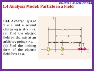
EX4: A charge +q is at
x = a and a second
charge –q is at x = -a.
(a) Find the electric
field on the axis at an
arbitrary point x > a.
(b) Find the limiting
form of the electric
field for x >> a.

Action of the Electric Field on charges
1. Electron moving parallel to a uniform electric field
EX5: An electron is
projected into a uniform
electric field E = 1000
(N/C) with an initial
velocity v0 = 2106 (m/s)
in the direction of the field.
How far does the electron
travel before it is brought
momentarily to rest?

2. Electron moving perpendicular to a uniform electric
field
EX6: An electron enters a uniform
electric field E = 2000 (N/C) with
an initial velocity v0 = 1106 (m/s)
perpendicular to the field.
(a) Compare the gravitational
force acting on the electron to the
electric force acting on it.
(b) By how much has the electron
been deflected after it has traveled
1.0 cm in the x direction?
Action of the Electric Field on charges

 Electric field due to a continuous
charge distribution
𝑬 = 𝑘𝑒
𝑖
Δ𝑞𝑖
𝑟𝑖
2 𝑟𝑖 = 𝒌𝒆
𝒅𝒒
𝒓𝟐
𝒓
1.5 Electric Field of a Continuous Charge
Distribution

1. Continuous Sources: Charge density
Distribution

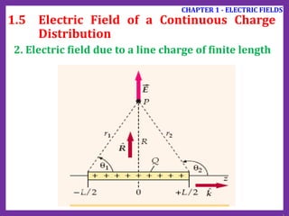
2. Electric field due to a line charge of finite length
EX7: A charge Q is uniformly distributed along the z axis,
from z = -L/2 to z = L/2. Show that for large value of z the
expression for the electric field of the line charge on the z
axis approaches the expression for the electric field of
a point charge Q at the origin
Distribution

EX8: A charge Q is uniformly distributed along the z axis,
from z=-L/2 to z=L/2.
(a) Find an expression for the electric field on the z=0
plane as a function of R, the radial distance of the field
point from the axis.
(b) Show that for R>>L, the expression found in Part (a)
approaches that of a point charge at the origin of charge
Q.
(c) Show that for the expression found in Part (a)
approaches that of an infinitely long line charge on the
axis with a uniform linear charge density =Q/L.
Distribution

Distribution

3. Electric field on the axis of a charged ring.
EX9: A thin ring (a circle)
of radius a is uniformly
charged with total charge
Q. Find the electric field
due to this charge at all
points on the axis
perpendicular to the
plane and through the
center of the ring.
Distribution

4. Electric field on the axis of a charged Disk.
EX10: Consider a uniformly charged thin disk of radius b
and surface charge density  ,
(a) Find the electric field at all points on the axis of the
disk.
(b) Show that for points on the axis and far from the disk,
the electric field approaches that of a point charge at the
origin with the same charge as the disk.
(c) Show that for a uniformly charged disk of infinite
radius, the electric field is uniform throughout the region
on either side of the disk.
Distribution

 When a particle of charge q and mass m is placed in an electric
field 𝑬, the electric force exerted on the charge is q𝑬. If that is
the only force exerted on the particle, it must be the net force,
and it causes the particle to accelerate. Therefore,
𝑭𝒆 = 𝒒𝑬 = m𝒂
→ 𝒂 =
𝒒𝑬
𝑚
 If 𝑬 is uniform (that is, constant in magnitude and direction) →
the particle under constant acceleration model to the motion
of the particle.
 If q >0, its acceleration is in the direction of the electric field.
 If q <0, its acceleration is in the direction opposite the electric
field.
1.7 Motion of a Charged Particle in a
Uniform Electric Field

CHAPTER 2 (2)
GAUSS’S LAW
2.1 Electric Field Lines and
Electric Flux
2.2 Gauss’s Law
2.3 Application of Gauss’s
Law to Various Charge
Distributions
2.4 Conductors in
Electrostatic Equilibrium

 Electric field vector 𝑬 and Electric field lines
Electric field lines (used to visualize
electric field patterns) are related to
the electric field:
 The electric field vector 𝐸 is tangent
to the electric field line at each point.
 The direction of the electric field line
is the same as of 𝐸.
 The number of lines per unit area
through a surface perpendicular to
the lines is proportional to the
magnitude of the electric field in that
region.
Pitfall Prevention:
Electric Field lines are
not Paths of Particles.
2.1 Electric Field Lines and Electric Flux
CHAPTER 2: GAUSS’S LAW

The rules for drawing electric field lines:
 The lines must begin on a positive
charge and terminate on a negative
charge. In the case of an excess of one
type of charge, some lines will begin
or end infinitely far away.
 The number of lines drawn leaving a
positive charge or approaching a
negative charge is proportional to the
magnitude of the charge.
 No two field lines can cross.

(a) The electric field lines for two point charges of equal magnitude and
opposite sign (an electric dipole). The number of lines leaving the positive
charge equals the number terminating at the negative charge. (b) The dark
lines are small pieces of thread suspended in oil, which align with the electric
field of a dipole.

(a) The electric field lines for two positive point charges. (b) Pieces of thread
suspended in oil, which align with the electric field created by two equal-
magnitude positive charges.

The electric field lines for
a point charge +2q and a
second point charge -q.

Rank the magnitudes of
the electric field at points
A, B, and C (greatest
magnitude first).

 Electric flux: 𝚽𝐄 = 𝑬. 𝑨
where E is the magnitude of
electric field
A is the surface area
perpendicular to the field
𝚽𝐄 is proportional to the
number of electric field
lines that penetrate
surface.
A
𝑬

 If electric field is uniform, electric
flux of 𝐸 through an area 𝐴:
𝚽𝑬 = 𝑬𝑨⊥ = 𝑬. 𝒏𝑨 = 𝑬𝑨 𝐜𝐨𝐬 𝜽
where 𝐴⊥ is a projection of area 𝐴
onto a plane oriented
perpendicular to the field, and 𝜃 =
𝐴, 𝐴⊥ ≡ 𝐸, 𝑛 with 𝑛 is the
normal vector of 𝐴.
 The general definition of electric
flux:
𝚽𝑬 =
𝐬𝐮𝐫𝐟𝐚𝐜𝐞
𝑬. 𝒅𝑨
where 𝑑𝐴 = 𝑛𝑑𝐴
(𝑵 ∙ 𝒎𝟐/C)

 Electric flux 𝚽𝐄
Note:
1. The dependence of electric
flux on the direction of 𝒏:
• 𝜽 < 𝟗𝟎°: 𝚽𝑬 > 𝟎
• 𝜽 > 𝟗𝟎°: 𝚽𝑬 < 𝟎
• 𝜽 = 𝟗𝟎°: 𝚽𝑬 = 𝟎
2. Convention of direction of the
area vector in the case of a
closed area: point outward from
the surface

Suppose a point charge is located at the center of a spherical
surface. The electric field at the surface of the sphere and the
total flux through the sphere are determined. Now the radius of
the sphere is halved. What happens to the flux through the
sphere and the magnitude of the electric field at the surface of
the sphere?
(a) The flux and field both increase.
(b) The flux and field both decrease.
(c) The flux increases, and the field decreases.
(d) The flux decreases, and the field increases.
(e) The flux remains the same, and the field increases.
(f) The flux decreases, and the field remains the same.

Example 2.1
Consider a uniform electric field 𝐸 oriented in the x direction in
empty space. A cube of edge length 𝑙, is placed in the field, oriented
as shown in the figure. Find the net electric flux through the surface
of the cube.

Example 2.1

2.2 Gauss’s Law

Gauss’s law:
𝚽𝑬 =
𝑺
𝑬. 𝒅𝑨 =
𝒒𝐢𝐧
𝝐𝟎
where 𝑞in is the net charge inside the closed surface 𝑆 (called
gaussian surface)
The net flux
through any
closed surface
surrounding a
point charge 𝑞 is
given by 𝑞/𝜖0 and
is independent of
the shape of that
surface.
2.2 Gauss’s Law

Determine the net
flux through the
surfaces S, S’, and S’’.
2.2 Gauss’s Law

2.2 Gauss’s Law
If the net flux through a gaussian surface is zero, the following
four statements could be true. Which of the statements must be
true?
(a) There are no charges inside the surface.
(b) The net charge inside the surface is zero.
(c) The electric field is zero everywhere on the surface.
(d) The number of electric field lines entering the surface equals
the number leaving the surface.

Gauss’s law is useful for determining electric fields when the
charge distribution is highly symmetric so that we can choose a
gaussian surface satisfying one or more of the following
conditions:
1. The value of the electric field can be argued by symmetry to be
constant over the portion of the surface.
2. 𝐸 and 𝑑𝐴 are parallel → Φ𝐸 = 𝑆
𝐸. 𝑑𝐴
3. 𝐸 and 𝑑𝐴 are perpendicular over a portion of the surface.
4. The electric field is zero over the portion of the surface.
2.3 Application of Gauss’s Law to Various Charge
Distributions
Note: Gaussian Surfaces Are not Real
A gaussian surface is an imaginary surface you construct to satisfy
the conditions listed here. It does not have to coincide with a
physical surface in the situation.

Distributions

Example 2.2
An insulating solid sphere of radius 𝑎 has a uniform volume charge
density 𝜌 and carries a total positive charge 𝑄.
(A) Calculate the magnitude of the electric field at a point outside the
sphere.
(B) Find the magnitude of the electric field at a point inside the
sphere.
Distributions

Example 2.2
(A) Calculate the magnitude of the electric field
at a point outside the sphere.
Distributions

Example 2.2
(B) Find the magnitude of the electric
field at a point inside the sphere.
Distributions

Example 2.3
Find the electric field a distance 𝑟 from a line of positive charge of
infinite length and constant charge per unit length 𝜆.
Distributions

Example 2.3
 Because the charge is distributed
uniformly along the line, the charge
distribution has cylindrical
symmetry and we can apply Gauss’s
law to find the electric field.
 The symmetry of the charge
distribution requires that 𝐸 be
perpendicular to the line charge and
directed outward as shown in the
figure.
Distributions
 To reflect the symmetry of the charge distribution, let’s choose a cylindrical
gaussian surface of radius r and length ℓ, that is coaxial with the line
charge. For the curved part of this surface, 𝐸 is constant in magnitude and
perpendicular to the surface at each point, satisfying conditions (1) and (2).
Furthermore, the flux through the ends of the gaussian cylinder is zero
because 𝐸 is parallel to these surfaces. That is the first application we have
seen of condition (3).

Example 2.3
Distributions

Example 2.5
Find the electric field due to an infinite plane of positive charge
with uniform surface charge density 𝜎.
Distributions

Example 2.6
Can Gauss’s law be used to calculate the electric field near an
electric dipole, a charged disk, or a triangle with a point charge at
each corner.?
Distributions

A conductor in electrostatic equilibrium (no net motion of
charge within a conductor) has the following properties:
1. The electric field is zero everywhere inside the conductor,
whether the conductor is solid or hollow.
2. If the conductor is isolated and carries a charge, the charge
resides on its surface.
3. The electric field at a point just outside a charged conductor is
perpendicular to the surface of the conductor and has a
magnitude 𝜎/𝜖0, where 𝜎 is the surface charge density at that
point.
4. On an irregularly shaped conductor, the surface charge density
is greatest at locations where the radius of curvature of the
surface is smallest.
2.4 Conductors in Electrostatic Equilibrium

CHAPTER 3 (3)
ELECTRIC POTENTIAL
3.1 Electric Potential and Potential
Difference
3.2 Potential Difference in a Uniform
Electric Field
3.3 Electric Potential and Potential
Energy Due to Point Charges
3.4 Obtaining the Value of the Electric
Field from the Electric Potential
3.5 Electric Potential Due to
Continuous Charge Distributions
3.6 Electric Potential Due to a Charged
Conductor

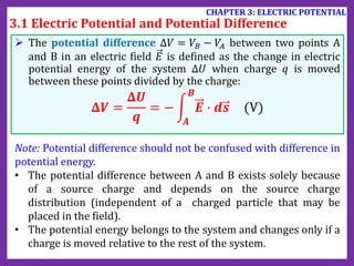
 When a positive charge 𝑞 is moved between points A and B in an
electric field 𝐸, the change in the potential energy of the
charge-field system is
𝚫𝑼 = −𝒒
𝑨
𝑩
𝑬 ⋅ 𝒅𝒔
 An equipotential surface is the surface on which all points are at
the same electric potential. Equipotential surfaces are
perpendicular to electric field lines.
 The electric potential that is characteristic of the field only is
determined by dividing the potential energy by the charge:
𝑽 =
𝑼
𝒒
(unit: J/C ≡ Volt)
3.1 Electric Potential and Potential Difference
CHAPTER 3: ELECTRIC POTENTIAL

 The potential difference Δ𝑉 = 𝑉𝐵 − 𝑉𝐴 between two points A
and B in an electric field 𝐸 is defined as the change in electric
potential energy of the system Δ𝑈 when charge 𝑞 is moved
between these points divided by the charge:
𝚫𝑽 =
𝚫𝑼
𝒒
= −
𝑨
𝑩
𝑬 ⋅ 𝒅𝒔 (V)
Note: Potential difference should not be confused with difference in
potential energy.
• The potential difference between A and B exists solely because
of a source charge and depends on the source charge
distribution (independent of a charged particle that may be
placed in the field).
• The potential energy belongs to the system and changes only if a
charge is moved relative to the rest of the system.

 The SI unit of electric field (N/C)
can also be expressed in volts per
meter:
1 N/c = 1 V/m
 The electric field is a measure of the
rate of change of the electric
potential with respect to position.

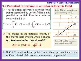
 The potential difference between two points
separated by a distance 𝑑 in a uniform electric
field 𝐸 is
➡ 𝚫𝑽 = −𝑬𝒅
if the direction of travel between the points is in
the same direction as the electric field.
The negative sign indicates that 𝑉𝐵 < 𝑉𝐴 →
Electric field lines always point in the
direction of decreasing electric potential.
 The change in the potential energy of the charge–field system when a
charge 𝒒 > 𝟎 moves in the direction of 𝑬:
𝚫𝑼 = 𝒒𝚫𝑽 = −𝒒𝑬𝒅
3.2 Potential Difference in a Uniform Electric Field

 The potential difference between two
points separated by vector 𝑠 that is not
parallel to the field lines in a uniform
electric field 𝐸 is
 The change in the potential energy of
the charge–field system when a charge
𝒒 > 𝟎 moves in the direction of 𝑬:
𝚫𝑼 = 𝒒𝚫𝑽 = −𝒒𝑬 ∙ 𝒔
3.2 Potential Difference in a Uniform Electric Field
 If 𝑬 ⊥ 𝒔 → 𝜟𝑽 = 0: all points in a plane perpendicular to a
uniform electric field are at the same electric potential.

3.3 Electric Potential and Potential Energy Due to
Point Charges

 If we define 𝑽 = 𝟎 at 𝒓 = ∞, the electric
potential due to a point charge at any
distance 𝑟 from the charge is
𝑽 = 𝒌𝒆
𝒒
𝒓
→ The electric potential due to a finite
number of point charges:
𝑽 = 𝒌𝒆
𝒊
𝒒𝒊
𝒓𝒊
 The potential difference between points A and B due to a point
charge 𝑞 depends only on the initial and final radial coordinates 𝑟𝐴
and 𝑟𝐵:
𝐕𝐁 − 𝐕𝐀 = 𝒌𝒆𝒒
𝟏
𝒓𝑩
−
𝟏
𝒓𝑨
Point Charges

 The electric potential energy associated
with a pair of point charges separated by
a distance
𝑼𝟏𝟐 = 𝑼𝟐𝟏 = 𝒌𝒆
𝒒𝟏𝒒𝟐
𝒓𝟏𝟐
→ We obtain the potential energy of a
distribution of point charges by
summing terms over all pairs of
particles.
E.g.: The total potential energy of the
system of three charges
𝑼 = 𝒌𝒆
𝒒𝟏𝒒𝟐
𝒓𝟏𝟐
+
𝒒𝟏𝒒𝟑
𝒓𝟏𝟑
+
𝒒𝟐𝒒𝟑
𝒓𝟐𝟑
Point Charges

➡ Electrostatic potential energy of a system of point charges
Point Charges

Example 3.1
As shown in the Fig. a, a charge 𝑞1 =
2.00 𝜇C is located at the origin and a
charge 𝑞2 = −6.00 𝜇C is located at (0,
3.00) m.
(A) Find the total electric potential
due to these charges at the point P,
whose coordinates are (4.00, 0) m.
(B) Find the change in potential
energy of the system of two
charges plus a third charge 𝑞 =
3.00 𝜇C as the latter charge moves
from infinity to point P (Fig. b).
Point Charges

Example 3.1
(A) Find the total electric potential due to
these charges at the point P, whose
coordinates are (4.00, 0) m.
Point Charges

Example 3.1
(B) Find the change in potential energy of the
system of two charges plus a third charge
𝑞 = 3.00 𝜇C as the latter charge moves
from infinity to point P (Fig. b).
Point Charges

The potential difference 𝑑𝑉 between two points a distance 𝑑𝑠 apart
can be expressed as 𝒅𝑽 = −𝑬 ⋅ 𝒅𝒔
 If the electric potential is known as a function of coordinates 𝑥,
𝑦, and 𝑧, we can obtain the components of the electric field by
taking the negative derivative of the electric potential with
respect to the coordinates:
𝑬𝒙 = −
𝒅𝑽
𝒅𝒙
, 𝑬𝒚 = −
𝒅𝑽
𝒅𝒚
, 𝑬𝒛 = −
𝒅𝑽
𝒅𝒛
3.4 Obtaining the Value of the Electric Field from the
Electric Potential
 If the charge distribution creating an electric field has spherical
symmetry such that the volume charge density depends only on
the radial distance 𝑟, the electric field is radial:
𝑬𝒓 = −
𝒅𝑽
𝒅𝒓

3.4 Obtaining the Value of the Electric Field from the
Electric Potential

 Calculate E
 𝚫𝑽 = − 𝑨
𝑩
𝑬 ⋅ 𝒅𝒔 between any two points
 Set V = 0 at some convenient points
3.5 Electric Potential Due to Continuous Charge
Distributions
Method 1
Method 2
The electric potential due to a continuous
charge distribution is
𝑽 = 𝒅𝑽 = 𝒌𝒆
𝒅𝒒
𝒓
Volume distribution: 𝑉 = 𝑘𝑒 𝜌𝑑𝑉/𝑟
Surface distribution: 𝑉 = 𝑘𝑒 𝜎𝑑𝐴/𝑟
Linear distribution: 𝑉 = 𝑘𝑒 𝜆𝑑𝑙/𝑟

Example 3.2
(A) Find an expression for the electric potential at a point P located
on the perpendicular central axis of a uniformly charged ring of
radius a and total charge 𝑄.
(B) Find an expression for the magnitude of the electric field at
point P.
Distributions

Example 3.2
(A) Find an expression for the electric potential at
a point P located on the perpendicular central
axis of a uniformly charged ring of radius a
and total charge 𝑄.
Distributions

Example 3.2
(B) Find an expression for the magnitude of the
electric field at point P.
Distributions

Example 3.3
A uniformly charged disk has radius R and surface charge density 𝜎.
(A) Find the electric potential at a point P along the perpendicular
central axis of the disk.
(B) Find the x component of the electric field at a point P along the
perpendicular central axis of the disk.
Distributions

Example 3.3
(A) Find the electric potential at a point P
along the perpendicular central axis of
the disk.
Distributions

Example 3.3
(B) Find the x component of the electric
field at a point P along the
perpendicular central axis of the disk.
Distributions

Example 3.4
A rod of length 𝑙, located along the 𝑥
axis has a total charge 𝑄 and a
uniform linear charge density 𝜆 .
Find the electric potential at a point
P located on the 𝑦 axis a distance 𝑎
from the origin.
Distributions

Example 3.4
Distributions

Every point on the surface of a
charged conductor in
electrostatic equilibrium is at
the same electric potential.
The potential is constant
everywhere inside the conductor
and equal to its value at the
surface.
3.6 Electric Potential Due to a Charged Conductor

Example 3.5
Two spherical conductors of radii r1 and
r2 are separated by a distance much
greater than the radius of either sphere.
The spheres are connected by a
conducting wire as shown in the figure.
The charges on the spheres in
equilibrium are q1 and q2 , respectively,
and they are uniformly charged. Find the
ratio of the magnitudes of the electric
fields at the surfaces of the spheres.
Distributions

Example 3.5
Distributions

CHAPTER 4 (1)
CAPACITANCE AND DIELECTRICS
4.1. Capacitance
4.2. Energy Stored in a
Charged Capacitor
4.3. Capacitors with
Dielectrics

Note: The capacitance depends only on the geometry of the
conductors and not on an external source of charge or potential
difference.
 Definition of capacitance
 A capacitor consists of two
conductors carrying charges of
equal magnitude and opposite sign.
 The capacitance 𝐶 of a capacitor is
defined as the ratio of the
magnitude of the charge on either
conductor to the magnitude of the
potential difference between the
conductors:
𝑪 =
𝑸
𝚫𝑽
(unit: C/V ≡ F)
4.1 Capacitance
CHAPTER 4: CAPACITANCE AND DIELECTRICS

 Definition of capacitance
4.1 Capacitance
1 𝐹 = 1
𝐶
𝑉
1μ𝐹 = 10−6
𝐹
1𝑝𝐹 = 10−12
𝐹

4.1 Capacitance

4.1 Capacitance
A capacitor stores charge Q at a potential difference ΔV. What
happens if the voltage applied to the capacitor by a battery is
doubled to 2ΔV?
(a) The capacitance falls to half its initial value, and the charge
remains the same.
(b) The capacitance and the charge both fall to half their initial
values.
(c) The capacitance and the charge both double.
(d) The capacitance remains the same, and the charge doubles.

 Isolated charged sphere
𝑪 =
𝑄
Δ𝑉
=
𝑄
𝑘𝑒𝑄/𝑎
=
𝑎
𝑘𝑒
= 𝟒𝝅𝝐𝟎𝒂
 Parallel-Plate capacitors
Δ𝑉 = 𝐸𝑑 =
𝜎
𝜖0
𝑑 =
𝑄𝑑
𝜖0𝐴
→ 𝑪 =
𝑄
Δ𝑉
=
𝝐𝟎𝑨
𝒅
 Cylindrical capacitor
𝑪 =
𝒍
𝟐𝒌𝒆𝐥𝐧(𝒃/𝒂)
 Spherical capacitor
𝑪 =
𝒂𝒃
𝒌𝒆(𝒃 − 𝒂)
 Calculating Capacitance
4.1 Capacitance

4.1 Capacitance
Many computer keyboard buttons are
constructed of capacitors as shown in
the figure. When a key is pushed down,
the soft insulator between the movable
plate and the fixed plate is
compressed. When the key is pressed,
what happens to the capacitance?
(a) It increases.
(b) It decreases.
(c) It changes in a way you cannot
determine because the electric
circuit connected to the key-board
button may cause a change in ΔV.

→ The equivalence capacitance in parallel combination:
𝑪𝒆𝒒 = 𝑪𝟏 + 𝑪𝟐 + 𝑪𝟑 + ⋯
Potential difference:
Δ𝑉 = Δ𝑉1 = Δ𝑉2
Total charge:
𝑄𝑡𝑜𝑡 = 𝑄1 + 𝑄2
= 𝐶1Δ𝑉1 + 𝐶2Δ𝑉2
= 𝐶1 + 𝐶2 ΔV
→ The equivalence
capacitance:
𝐶𝑒𝑞 = 𝐶1 + 𝐶2
 Parallel combination
 Combinations of Capacitors
4.1 Capacitance

→ The equivalence capacitance:
𝟏
𝑪𝒆𝒒
=
𝟏
𝑪𝟏
+
𝟏
𝑪𝟐
+
𝟏
𝑪𝟑
+ ⋯
Charge on capacitors:
𝑄1 = 𝑄2 = 𝑄
Δ𝑉𝑡𝑜𝑡 = Δ𝑉1 + Δ𝑉2
=
1
𝐶1
+
1
𝐶2
𝑄
→ The equivalence
capacitance:
1
𝐶𝑒𝑞
=
1
𝐶1
+
1
𝐶2
 Series combination
 Combinations of Capacitors
4.1 Capacitance

4.1 Capacitance
Two capacitors are identical. They can be connected in series or
in parallel. If you want the smallest equivalent capacitance for
the combination, how should you connect them
(a) in series
(b) in parallel
(c) either way because both combinations have the same
capacitance

The potential energy stored in a charged capacitor:
𝑼𝑬 =
𝑸𝟐
𝟐𝑪
=
𝟏
𝟐
𝑸𝚫𝑽 =
𝟏
𝟐
𝑪 𝚫𝑽 𝟐
4.2 Energy Stored in a Charged Capacitor

4.2 Energy Stored in a Charged Capacitor
You have three capacitors and a battery. In which of the following
combinations of the three capacitors is the maximum possible
energy stored when the combination is attached to the battery?
(a) series
(b) parallel
(c) no difference because both combinations store the same
amount of energy

When a dielectric material is inserted between the plates of a
capacitor, the capacitance increases by a dimensionless factor 𝜿,
called the dielectric constant:
𝑪 = 𝜿𝑪𝟎
+ Potential difference
of a capacitor without
dielectric: Δ𝑉0
+ Potential difference
of a capacitor with
dielectric:
Δ𝑉 =
Δ𝑉0
𝜅
→ Capacitance
𝑪 =
𝑸𝟎
𝚫𝑽
= 𝜿
𝑸𝟎
𝚫𝑽𝟎
= 𝜿𝑪𝟎
4.3 Capacitors with Dielectrics

CHAPTER 5 (3)
ELECTRIC CURENT AND DIRECT-CURRENT CIRCUITS
5.1. Electric current and motion of
charge
5.2. Resistance and Ohm's Law
5.3. Electromotive Force
5.4. Resistors in Series and Parallel
5.5. Kirchhoff’s Rules
5.6. Power
5.7. RC Circuits

5.1 Electric current and motion of charge
CHAPTER 5: DIRECT-CURRENT CIRCUITS

5.1 Electric current and motion of charge
Microscopic Model of Current
(a) A schematic diagram of the random
motion of two charge carriers in a conductor
in the absence of an electric field. The drift
velocity is zero.
(b) The motion of the charge carriers in a
conductor in the presence of an electric field.

5.2 Resistance and Ohm's Law

5.2 Resistance and Ohm's Law
For many materials (including most
metals), the ratio of the current
density to the electric field is a
constant σ that is independent of
the electric field producing the
current.

 Direct current (DC): the current in the circuit is constant in
magnitude and direction
 Battery: a source of energy for circuits or a source of
electromotive force (emf, 𝓔)
 The emf 𝓔 of a battery: the maximum possible voltage the
battery can provide between its terminals
 Internal resistance (𝒓): resistance to the flow of charge
within the battery
 Load resistance (𝑹): resistance of some electrical device
connected to the battery
5.3 Electromotive Force

Electromotive force (emf, 𝓔) of a battery is equal to the
voltage across its terminals when the current is zero (or the
open-circuit voltage of the battery)

5.4 Resistors in Series and Parallel

The equivalence resistor: 𝑹𝒆𝒒 = 𝑹𝟏 + 𝑹𝟐 + ⋯
 Series combinations
Current:
𝐼 = 𝐼1 = 𝐼2
Δ𝑈 = Δ𝑈1 + Δ𝑈2 → 𝐼𝑅𝑒𝑞 = 𝐼1𝑅1 + 𝐼2𝑅2

The equivalence resistor:
𝟏
𝑹𝒆𝒒
=
𝟏
𝑹𝟏
+
𝟏
𝑹𝟐
+ ⋯
Potential difference: Δ𝑈 = Δ𝑈1 = Δ𝑈2
Current:
𝐼 = 𝐼1 + 𝐼2 →
Δ𝑈
𝑅𝑒𝑞
=
Δ𝑈1
𝑅1
+
Δ𝑈2
𝑅2
 Parallel combinations

 Junction rule: At any junction, the sum of the currents must equal zero
𝐣𝐮𝐧𝐜𝐭𝐢𝐨𝐧
𝑰 = 𝟎
𝑰𝟏 − 𝑰𝟐 − 𝑰𝟑 = 𝟎
5.5 Kirchhoff’s Rules

 Loop rule: The sum of the potential differences across all elements
around any closed circuit loop must be zero
𝐜𝐥𝐨𝐬𝐞𝐝 𝐥𝐨𝐨𝐩
𝚫𝑼 = 𝟎
𝚫𝑽 = 𝑽𝒃 − 𝑽𝒂

Example 5.1
A single-loop circuit contains two
resistors and two batteries as
shown in the figure. (Neglect the
internal resistances of the
batteries.) Find the current in the
circuit.

Example 5.2
Find the currents 𝐼1, 𝐼2, 𝐼3 in the circuit shown in the figure.

Ex. 1 1 =12(V), 2 =11(V), the internal resistances of the
batteries are r1 = r2 =0,02, and the load resistance R = 0,01.
What will be the charging current?

EX. 2 Find the current in each branch of the circuit shown in
figure.

EX. 3 Find the current in each branch of the circuit shown in
figure.

5.6 Power

Ohm law: 𝚫𝑽 = 𝓔 − 𝑰𝒓 = 𝑰𝑹 → 𝓔 = 𝑰(𝑹 + 𝒓)
Power delivered by a battery: 𝑷 = 𝑰𝓔 = 𝑰𝟐
(𝑹 + 𝒓)
5.6 Power

5.7 RC circuits

5.7 RC circuits
Charging a capacitor

CHAPTER 6 (3)
MAGNETIC FIELDS
6.1 Analysis Model: Particle in a
Field (Magnetic)
6.2 Motion of a Charged Particle
in a Uniform Magnetic Field
6.3 Applications Involving
Charged Particles Moving in a
Magnetic Field
6.4 Magnetic Force Acting on a
Current-Carrying Conductor
6.5 Torque on a Current Loop in a
Uniform Magnetic Field

In addition to containing an electric field, the region of space
surrounding any moving electric charge also contains a
magnetic field (characterized by magnetic field vector 𝐵)
6.1 Particle in a Magnetic Field
CHAPTER 6: MAGNETIC FIELDS

When a particle with charge 𝑞 and moving with velocity 𝑣 is placed
in a magnetic field 𝐵, it experiences a magnetic force given by
𝑭𝑩 = 𝒒𝒗 × 𝑩 → 𝑭𝑩 = 𝒒 𝒗𝑩 𝐬𝐢𝐧𝜽

Using the right-hand rule to determine the direction of 𝒗 × 𝑩

 𝒗 perpendicular to 𝑩
 𝐹𝑩 ⊥ (𝑣, 𝐵) → particle moves in a
circular path in a plane perpendicular
to 𝐵 under 𝐹𝑩
 𝐹𝐵 = 𝑞𝑣𝐵 = const → uniform circular
motion
• Radius of the circular path
𝑟 = 𝑚𝑣/𝑞𝐵
• Angular speed
𝜔 = 𝑣/𝑟 = 𝑞𝐵/𝑚
• Period of the motion
𝑇 = 2𝜋/𝜔 = 2𝜋𝑚/𝑞𝐵
𝑭𝑩 = 𝒒𝒗 × 𝑩

 𝒗 at some angle with respect to 𝑩
 In 𝑥 direction: 𝐹𝑥 = 0 → 𝒗𝒙 = 𝐜𝐨𝐧𝐬𝐭
 Projection onto the 𝑦𝑧 plane:
uniform circular motion under 𝐹𝐵
• Radius of the circular path
𝑟 = 𝑚𝑣⊥/𝑞𝐵
• Angular speed
𝜔 = 𝑣⊥/𝑟 = 𝑞𝐵/𝑚
• Period of the motion
𝑇 = 2𝜋/𝜔 = 2𝜋𝑚/𝑞𝐵
⟹ The particle moves in a helical
path
𝐵 = 𝐵𝑖
𝑣 = 𝑣𝑥𝑖 + 𝑣𝑦𝑗 + 𝑣𝑧𝑘
= 𝑣𝑥𝑖 + 𝑣⊥
→ 𝐹𝐵 = 𝑞𝑣 × 𝐵
= 𝑞𝑣⊥ × 𝐵
(𝐹𝐵 ⊥ 𝐵, 𝑣⊥ = 𝑣𝑦
2
+ 𝑣𝑧
2)

Video demonstrates for a charged particle in a uniform magnetic field

EX. 1: An electron moves in a circular path perpendicular
to a uniform magnetic field with a magnitude of 2.00 mT.
If the speed of the electron is 1.50  107 m/s, determine
(a) the radius of the circular path and
(b) the time interval required to complete one revolution.

EX. 2: Determine the initial direction of the deflection of
charged particles as they enter the magnetic fields shown in
the figure.

The total force (called the Lorentz force)
acts on a charge moving with a velocity 𝑣
in the presence of both 𝐸 and 𝐵:
𝑭 = 𝒒𝑬 + 𝒒𝒗 × 𝑩
 𝐕𝐞𝐥𝐨𝐜𝐢𝐭𝐲 𝐒𝐞𝐥𝐞𝐜𝐭𝐨𝐫
The magnitudes of 𝑬 and 𝑩 are chosen so
that
𝒒𝑬 = 𝒒𝒗𝑩 → 𝑣 =
𝐸
𝐵
→ only those particle having this speed
pass undeflected through the mutually
perpendicular electric and magnetic fields
→ splitting beams with the same velocity
6.3 Applications Involving Charged Particles
Moving in a Magnetic Field

 𝐓𝐡𝐞 𝐌𝐚𝐬𝐬 𝐒𝐩𝐞𝐜𝐭𝐫𝐨𝐦𝐞𝐭𝐞𝐫
A beam of ions first passes through a
velocity selector (𝐸, 𝐵) and then enters a
second uniform magnetic field 𝐵0 (the
same direction as 𝐵).
When entering 𝐵0, the ions move in the
circular path under an magnetic force:
𝑚
𝑣2
𝑟
= 𝑞𝑣𝐵0 →
𝑚
𝑞
=
𝑟𝐵0
𝑣
=
𝑟𝐵0𝐵
𝐸
where 𝑣 = 𝐸/𝐵 (via the velocity
selector)
→ determining the ratio 𝒎/𝒒 by
measuring 𝒓 and knowing 𝑩, 𝑬, 𝑩𝟎

 𝐓𝐡𝐞 𝐂𝐲𝐜𝐥𝐨𝐭𝐫𝐨𝐧

Video about structure and operation principle of a cyclotron

6.4 Magnetic Force Acting on a Current-
Carrying Conductor

The magnetic
force exerted on a
small segment 𝑑𝑠:
𝒅𝑭𝑩 = 𝑰𝒅𝒔 × 𝑩
The total magnetic force acting on the wire:
𝑭𝑩 =
𝑨
𝑩
𝑰𝒅𝒔 × 𝑩
Carrying Conductor
𝑭𝑩 = 𝑰𝑳 × 𝑩

Example 6.1
A wire bent into a semicircle of
radius 𝑅 forms a closed circuit
and carries a current 𝐼. The wire
lies in the 𝑥𝑦 plane, and a
uniform magnetic field is
directed along the positive y
axis as in the Figure. Find the
magnitude and direction of the
magnetic force acting on the
straight portion of the wire and
on the curved portion.
Carrying Conductor

Example 6.1
Carrying Conductor

Consider a rectangular loop carrying a current 𝐼 in the presence of
a uniform magnetic field directed parallel to the plane
6.5 Torque on a Current Loop in a Uniform
Magnetic Field

Magnetic Field
The torque 𝝉 on a current loop placed in a uniform magnetic
field 𝑩 is
𝝉 = 𝝁 × 𝑩
where 𝝁 = 𝑰𝑨 is the magnetic dipole moment of the loop

Magnetic Field

CHAPTER 7 (3)
SOURCES OF THE MAGNETIC FIELD
7.1 The Biot–Savart Law
7.2 The Magnetic Force Between Two Parallel Conductors
7.3 Ampère’s Law
7.4 The Magnetic Field of a Solenoid
7.5 Gauss’s Law in Magnetism

3
 Biot-Savart law: The magnetic field 𝒅𝑩 at a point P associated
with a length element 𝒅𝒔 of a wire carrying a steady current 𝑰
𝒅𝑩 =
𝝁𝟎
𝟒𝝅
𝑰𝒅𝒔 × 𝒓
𝒓𝟐
 𝑑𝐵 is perpendicular both to
𝑑𝑠 (pointing in the direction
of the current) and 𝑟 (unit
vector directed from 𝑑𝑠 to P)
 The direction of 𝑑𝐵 is
determined by the right-
hand rule
 The magnitude of 𝑑𝐵:
𝒅𝑩 =
𝝁𝟎
𝟒𝝅
𝑰𝒅𝒔
𝒓𝟐
Permeability of free space
𝜇0 = 4𝜋 × 10−7
T. m/A
CHAPTER 7: SOURCES OF THE MAGNETIC FIELD

4
The right-hand rule for
determining the direction
of the magnetic field
surrounding a long,
straight wire carrying a
current. Positioning the
thumb along the direction
of the current, the four
fingers wrap in the
direction of the magnetic
field. Notice that the
magnetic field lines form
circles around the wire.

5
 Biot-Savart law: The magnetic field 𝑩 at a point P due to a wire
carrying a steady current 𝑰
𝑩 =
𝝁𝟎
𝟒𝝅 𝐜𝐮𝐫𝐫𝐞𝐧𝐭
𝒓𝟐
Although the Biot–Savart law was discussed for a current-carrying
wire, it is also valid for a current consisting of charges flowing
through space such as the particle beam in an accelerator. In that
case, 𝒅𝒔 represents the length of a small segment of space in which
the charges flow.

6
Magnetic field due to a
current element
Electric field
due to a point charge
Equation
𝒅𝑩 =
𝝁𝟎
𝟒𝝅
𝒓𝟐
𝑬 = 𝒌𝒆
𝒒𝒓
𝒓𝟐
Similarities The magnitude of the field varies as the inverse square
of the distance from the source
Differences
Direction is perpendicular to
both 𝒅𝒔 and 𝒓
Radial direction
only the first step in a
calculation of a magnetic
field; it must be followed by
an integration over the
current distribution
established by an
isolated electric charge

7

8
Consider the magnetic field due to the current in the wire shown in
Figure 7.2. Rank the points A, B, and C in terms of magnitude of the
magnetic field that is due to the current in just the length element
𝒅𝒔 shown from greatest to least.

9
Example 7.1
Consider a thin, straight wire of finite length carrying a constant
current 𝐼 and placed along the 𝑥 axis. Determine the magnitude and
direction of the magnetic field at point 𝑃 due to this current.

10
Example 7.1
Let’s start by considering a length
element 𝒅𝒔 located a distance r from
P. The direction of the magnetic field
at point P due to the current in this
element is out of the page because
𝒅𝒔 × 𝒓 is out of the page. In fact,
because all the current elements 𝑰𝒅𝒔
lie in the plane of the page, they all
produce a magnetic field directed
out of the page at point P. Therefore,
the direction of the magnetic field at
point P is out of the page and we
need only find the magnitude of the
field.

11
Example 7.1

12
Example 7.1

13
Example 7.2
Calculate the magnetic field at point O for the current-carrying wire
segment shown in Figure 7.4. The wire consists of two straight
portions and a circular arc of radius a, which subtends an angle θ.

14
Example 7.2

15
Example 7.2

16
Example 7.3
Consider a circular wire loop of radius 𝑎 located in the 𝑦𝑧-plane and
carrying a steady current 𝐼 as in the Figure. Calculate the magnetic
field at an axial point 𝑃 a distance 𝑥 from the center of the loop.

17
Example 7.3
Compare this problem to Example 23.8 for the electric field due to a ring of
charge. Figure 7.5 shows the magnetic field contribution 𝒅𝑩 at P due to a
single current element at the top of the ring. This field vector can be resolved
into components dBx parallel to the axis of the ring and dB⫠ perpendicular
to the axis. Think about the magnetic field contributions from a current
element at the bottom of the loop. Because of the symmetry of the situation,
the perpendicular components of the field due to elements at the top and
bottom of the ring cancel. This cancellation occurs for all pairs of segments
around the ring, so we can ignore the perpendicular component of the field
and focus solely on the parallel components, which simply add.

18
Example 7.3

Example 7.3

20
 Magnetic field at wire 2
from current in wire 1:
𝐵1 2 =
𝜇0𝐼1
2𝜋𝑟
 Force on a length Δ𝑙 of
wire 2:
Δ𝐹12 = 𝐼2Δ𝑙 𝐵1(2)
 Force per unit length in
terms of the current:
𝒇𝟏𝟐 =
𝚫𝑭
𝚫𝒍
=
𝝁𝒐𝑰𝟏𝑰𝟐
𝟐𝝅𝒂
7.2 The Magnetic Force Between Two
Parallel Conductors

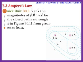
21
Ampere’s law: The line integral of 𝑩. 𝒅𝒔 around any closed path
(amperian loop) equals 𝝁𝟎𝑰, where I is the total steady current
passing through any surface bounded by the closed path:
𝒞
𝑩 ⋅ 𝒅𝒔 = 𝝁𝟎𝑰
Note: Sign of 𝑰 in Ampere’s law
When using Ampère’s law, apply the following right-hand rule.
 Point your thumb in the direction of the current through the
amperian loop.
 Your curled fingers then point in the direction that you should
integrate when traversing the loop to avoid having to define the
current as negative.
7.3 Ampère’s Law

22
7.3 Ampère’s Law

7.3 Ampère’s Law

24
Example 7.5
A long, straight wire of radius 𝑅
carries a steady current 𝐼 that is
uniformly distributed through
the cross section of the wire.
Calculate the magnetic field a
distance 𝑟 from the center of
the wire in the regions 𝑟 ≥ 𝑅
and 𝑟 < 𝑅.
7.3 Ampère’s Law

25
Example 7.5
 The current creates magnetic fields everywhere, both inside and outside the wire.
 Because the wire has a high degree of symmetry, we categorize this example as an Ampère’s
law problem. For the r ≥ R case, we should arrive at the same result as was obtained in Example
7.1, where we applied the Biot–Savart law to the same situation.
7.3 Ampère’s Law

Example 7.5
7.3 Ampère’s Law

Example 7.6
A device called a toroid is often
used to create an almost
uniform magnetic field in some
enclosed area. The device
consists of a conducting wire
wrapped around a ring (a
torus) made of a non-
conducting material. For a
toroid having 𝑁 closely spaced
turns of wire, calculate the
magnetic field in the region
occupied by the torus, a
distance 𝑟 from the center.
7.3 Ampère’s Law

Example 7.6
• Imagine each turn of the wire to be a circular loop as in Example 7.3. The
magnetic field at the center of the loop is perpendicular to the plane of the
loop. Therefore, the magnetic field lines of the collection of loops will form
circles within the toroid such as suggested by loop 1 in Figure 7.15.
• Because the toroid has a high degree of symmetry, we categorize this
example as an Ampère’s law problem.
• Consider the circular amperian loop (loop 1) of radius r in the plane of
Figure 7.15. By symmetry, the magnitude of the field is constant on this
circle and tangent to it, so 𝑩 ⋅ 𝒅𝒔 = 𝑩𝒅𝒔. Furthermore, the wire passes
through the loop N times, so the total current through the loop is NI.
• Apply Ampère’s law to loop 1:
7.3 Ampère’s Law

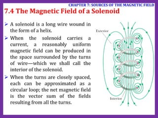
 A solenoid is a long wire wound in
the form of a helix.
 When the solenoid carries a
current, a reasonably uniform
magnetic field can be produced in
the space surrounded by the turns
of wire—which we shall call the
interior of the solenoid.
 When the turns are closely spaced,
each can be approximated as a
circular loop; the net magnetic field
is the vector sum of the fields
resulting from all the turns.

 An ideal solenoid: the turns are
closely spaced and the length is
much greater than the radius of the
turns. → The external field is close
to zero and the interior field is
uniform over a great volume.
 Interior magnetic field:
𝑩𝐢𝐧 =
𝝁𝟎𝑵𝑰
𝑳
= 𝝁𝟎𝒏𝑰
 Exterior magnetic field:
Applying the Ampere’s law, with the
amperian loop being the loop 2, we get
𝑩𝐨𝐮𝐭 = 𝟎

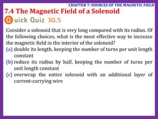
Consider a solenoid that is very long compared with its radius. Of
the following choices, what is the most effective way to increase
the magnetic field in the interior of the solenoid?
(a) double its length, keeping the number of turns per unit length
constant
(b) reduce its radius by half, keeping the number of turns per
unit length constant
(c) overwrap the entire solenoid with an additional layer of
current-carrying wire

 Gauss’s law in magnetism
The net magnetic flux through any closed surface is always zero:
𝚽𝑩 = 𝑩 ⋅ 𝒅𝑨 = 𝟎
 Magnetic flux 𝚽𝐁 through a surface 𝑆
𝚽𝑩 =
𝑺
𝑩 ⋅ 𝒅𝑨
7.5 Gauss’s Law in Magnetism

CHAPTER 8 (3)
FARADAY‘S LAW
8.1 Faraday’s Law of Induction
8.2 Motional emf
8.3 Lenz’s Law
8.4 Induced emf and Electric Fields
8.5 Generators and Motors

CHAPTER 8: FARADAY‘S LAW

Faraday’s law of induction
𝓔 = −
𝒅𝚽𝑩
𝒅𝒕
𝓔: induction emf; 𝚽𝐁 = 𝑩 ∙ 𝒅𝑨 : magnetic flux through the loop

 If a coil consists of N loops with the same area and 𝚽𝐁 is the
magnetic flux through one loop, an emf is induced in every loop.
 The loops are in series, so their emfs add; therefore, the total
induced emf in the coil is given by:
 Suppose a loop enclosing an area A lies
in a uniform magnetic field 𝑩 as in the
figure. The magnetic flux through the
loop is equal to BA cosθ, where θ is the
angle between the magnetic field and
the normal to the loop.
 The induced emf can be expressed as

Some application of Faraday’s law
(a)In an electric guitar, a vibrating magnetized
string induces an emf in a pickup coil.
(b)The pickups (the circles beneath the metallic
strings) of this electric guitar detect the
vibrations of the strings and send this
information through an amplifier and into
speakers.

A circular loop of wire is held in a uniform magnetic field, with the
plane of the loop perpendicular to the field lines. Which of the
following will not cause a current to be induced in the loop?
(a) crushing the loop
(b) rotating the loop about an axis perpendicular to the field lines
(c) keeping the orientation of the loop fixed and moving it along the
field lines
(d) pulling the loop out of the field

Motional emf (the emf induced in a conductor moving through a
constant magnetic field): When a conducting bar of length 𝒍, moves
at a velocity 𝒗 through a magnetic field 𝑩 , where 𝑩 is
perpendicular to the bar and to 𝒗, the motional emf induced in the
bar is
𝓔 = −𝑩𝒍𝒗
 Magnetic force 𝑭𝑩 = 𝒒𝒗 × 𝑩 makes the ends
of the conductor become oppositely charged.
→ Create an electric field 𝑬 in the conductor.
 In turn, the electric field 𝑬 acts on electrons
by the force 𝑭𝑬 = 𝒒𝑬, whose direction is
opposite to the direction of 𝑭𝑩.
 In equilibrium condition, 𝑭𝑩 = 𝑭𝑬 → 𝑬 = 𝒗𝑩
→ The potential different across the ends of the
conductor 𝚫𝑽 = 𝑬𝒍 = 𝑩𝒍𝒗.
8.2 Motional emf

Example 8.3
The conducting bar illustrated in the figure moves on two
frictionless, parallel rails in the presence of a uniform magnetic field
directed into the page. The bar has mass m, and its length is 𝑙. The
bar is given an initial velocity 𝑣i to the right and is released at 𝑡 = 0.
Using Newton’s laws, find the velocity of the bar as a function of
time.
8.2 Motional emf

Example 8.3
 As the bar slides to the right in the
figure, a counterclock-wise current is
established in the circuit consisting of
the bar, the rails, and the resistor. The
upward current in the bar results in a
magnetic force to the left on the bar as
shown in the figure. Therefore, the bar
must slow down, so our mathematical
solution should demonstrate that.
8.2 Motional emf
• We model the bar as a particle under a net force.
• From Equation 29.10 (chapter 29), the magnetic force is FB = -I 𝑙 B,
where the negative sign indicates that the force is to the left. The
magnetic force is the only horizontal force acting on the bar.

Example 8.3
8.2 Motional emf
Using the particle under a net force model, apply Newton’s second law to the bar
in the horizontal direction:

Example 8.3
8.2 Motional emf
• This expression for v indicates that the velocity of the bar decreases with time
under the action of the magnetic force as expected.

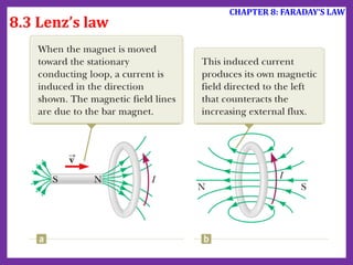
Lenz’s law: The induced current in a loop is in the direction that
creates a magnetic field that opposes the change in magnetic flux
through the area enclosed by the loop.
8.3 Lenz’s law

8.3 Lenz’s law

8.3 Lenz’s law
The below figure shows a circular
loop of wire falling toward a wire
carrying a current to the left. What
is the direction of the induced
current in the loop of wire?
(a) clockwise
(b) counterclockwise
(c) zero
(d) impossible to determine

General form of Faraday’s law:
𝑬 ⋅ 𝒅𝒔 = −
𝒅𝚽𝑩
𝒅𝒕
where 𝑬 is the nonconservative electric
field that is produced by the changing
magnetic flux.
Let consider a conducting loop in a
changing magnetic field:
 A changing magnetic flux through the
loop induces an emf and a current in it.
 According to definition of emf, we have
𝓔 = 𝑬 ⋅ 𝒅𝒔

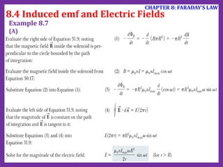
Example 8.7
A long solenoid of radius R has n turns
of wire per unit length and carries a
time varying current that varies
sinusoidally as 𝐼 = 𝐼𝑚𝑎𝑥 cos 𝜔𝑡, where
𝐼𝑚𝑎𝑥 is the maximum current and 𝜔 is
the angular frequency of the
alternating current source.
(A) Determine the magnitude of the
induced electric field outside the
solenoid at a distance 𝑟 > 𝑅 from
its long central axis.
(B) What is the magnitude of the
induced electric field inside the
solenoid, a distance r from its axis?

Example 8.7
(A)

Example 8.7
(B)

Generator
Electric generators are devices that
take in energy by work and transfer
it out by electrical transmission.
A coil with N turns, with the same
area A, rotates in a magnetic field
with a constant angular speed 𝜔:
𝓔 = −𝑵
𝒅𝚽𝑩
𝒅𝒕
= 𝑵𝑩𝑨 𝐬𝐢𝐧 𝝎𝒕
alternating-current (AC) generator

direct-current (DC) generator

Motor
A motor is a device into which energy
is transferred by electrical
transmission while energy is
transferred out by work.
A motor is essentially a generator
operating in reverse. Instead of
generating a current by rotating a coil,
a current is supplied to the coil by a
battery, and the torque acting on the
current-carrying coil causes it to
rotate.

INTERFERENCE OF LIGHT WAVES
CHAPTER 9 (3)
9.1 Conditions for Interference
9.2 Young’s Double-Slit Experiment
9.3 Intensity Distribution of the
Double-Slit Interference Pattern
9.4 Phasor Addition of Waves
9.5 Change of Phase Due to Reflection
9.6 Interference in Thin Films
9.7 The Michelson Interferometer

interference
pattern of
water waves
Light waves also interfere with one another,
like mechanical waves.
CHAPTER 9 – INTERFERENCE OF LIGHT WAVES

Conditions for
interference in light
waves:
• The sources must be
coherent.
• The sources should
be monochromatic;
that is, they should be
of a single wavelength
(or frequency).
Incoherent and coherent light sources:
• Incoherent light sources do not have the same frequency and
the waves are not in phase with one another.
• Coherent light sources possess the same frequency and their
waves are in phase with one another.

9.2 Young’sDouble-SlitExperiment
(a) If light waves did not
spread out after passing
through the slits, no
interference would occur.
(b) The light waves from the two slits
overlap as they spread out, filling what
we expect to be shadowed regions with
light and producing interference fringes
on a screen placed to the right of the slits.
Diffraction

Interference in light waves from two sources was first
demonstrated by Thomas Young in 1801.

Linear positions of bright and dark fringes:
𝜽 small: 𝐬𝐢𝐧 𝜽 ≈ 𝒚/𝑳 → 𝜹 ≈ 𝒚𝒅/𝑳

Which of the following will cause the fringes in a two-slit
interference pattern to move farther apart?
(a) decreasing the wavelength of the light
(b) decreasing the screen distance L
(c) decreasing the slit spacing d
(d) Immersing the entire apparatus in water.

Example 9.1:
A viewing screen is separated from a double slit by 1.2 m.
The distance between the two slits is 0.030 mm.
Monochromatic light is directed toward the double slit
and forms an interference pattern on the screen. The
second-order bright fringe is 4.50 cm from the center line
on the screen.
(a)Determine the wavelength of the light.
(b)Calculate the distance between adjacent bright
fringes.

Example 9.1:

Example 9.2:
A light source emits visible light of two wavelengths:
 = 430 nm and ’ = 510 nm. The source is used in a
double-slit interference experiment in which L = 1.50 m
and d = 0.025 mm.
a) Find the separation distance between the third-order
bright fringes for the two wavelengths.
b) Find the locations on the screen where the bright
fringes from the two wavelengths overlap exactly.

Example 9.2:
a) Find the separation distance between the third-order bright
fringes for the two wavelengths.

Example 9.2:
b) Find the locations on the screen where the bright fringes
from the two wavelengths overlap exactly.

Resultant wave at point P:
𝑬𝑷 = 𝟐𝑬𝟎 𝐜𝐨𝐬
𝚫𝝓
𝟐
𝐬𝐢𝐧(𝝎𝒕 +
𝝓𝟏 + 𝝓𝟐
𝟐
)
→ The light intensity at P:
𝑰𝑷 ∝ 𝑬𝑷
𝟐
𝐚𝐯𝐠
→
Two separated waves at point P:
𝐸1 = 𝐸0 sin(𝜔𝑡 + 𝜙1)
𝐸2 = 𝐸0 sin(𝜔𝑡 + Φ2)
where the phase difference:
Δ𝜙 =
2𝜋
𝜆
𝛿 =
2𝜋
𝜆
𝑑 sin 𝜃
Δ𝜙 ≈
𝟐𝝅
𝝀
𝒚𝒅
𝑳
(𝜃 small)
9.3. IntensityDistributionof theDouble-Slit
InterferencePattern

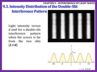
Light intensity versus
𝑑 sin𝜃 for a double-slit
interference pattern
when the screen is far
from the two slits
(L≫d).
9.3. IntensityDistributionof theDouble-Slit
InterferencePattern

9.4. PhasorAdditionof Waves
(a) Phasor diagram for the wave disturbance
𝑬𝟏 = 𝑬𝒐𝒔𝒊𝒏𝝎𝒕. The phasor is a vector of
length Eo rotating counterclockwise.
(b) Phasor diagram for the wave
𝑬𝟐 = 𝑬𝒐𝐬𝐢𝐧(𝝎𝒕 + 𝝓).
(c) The phasor ER represents the combination
of the waves in part (a) and (b).

Phasor diagrams for a double-slit interference pattern. The resultant phasor ER
is a maximum when 𝝓 = 𝟎, 𝟐𝝅, 𝟒𝝅, . . . and is zero when 𝝓 = 𝟎, 𝟑𝝅, 𝟓𝝅 , . . . .

Phasor diagrams for three equally
spaced slits at various values of 𝝓.

Multiple-slit interference
patterns. As N, the number
of slits, is increased, the
primary maxima (the
tallest peaks in each
graph) become narrower
but remain fixed in
position and the number
of secondary maxima
increases. For any value of
N, the decrease in
intensity in maxima to the
left and right of the central
maximum, indicated by
the blue dashed arcs, is
due to diffraction patterns
from the individual slits.

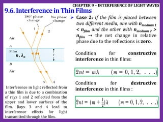
Interference pattern with a single light source (Lloyd’s mirror)
 Light waves can reach point P
on the screen either directly
from S to P or by the path
involving reflection from the
mirror.
 The reflected ray can be treated
as a ray originating from a
virtual source S’.
 Note: An electromagnetic wave
undergoes a phase change of
180° upon reflection from a
medium that has a higher
index of refraction than the
one in which the wave is
traveling.
9.5. Change of PhaseDue to Reflection
Lloyd’s mirror. An interference pattern
is produced at point P on the screen as
a result of the combination of the
direct ray (blue) and the reflected ray
(brown). The reflected ray undergoes
a phase change of 180°.

For n1 < n2 , a light ray traveling in medium 1 when reflected from
the surface of medium 2 undergoes a 180° phase change. The
same thing happens with a reflected pulse traveling along a string
fixed at one end.

For n1 > n2 , a light ray traveling in medium 1 undergoes no phase
change when reflected from the surface of medium 2. The same is
true of a reflected wave pulse on a string whose supported end is
free to move.

 Consider a film of uniform
thickness 𝒕 and refraction index 𝒏.
 Assuming that the light rays traveling
in air are nearly normal to the two
surfaces of the film.
 To determine whether the reflected
rays interfere constructively or
destructively, we first note the
following facts:
 n1 < n2: a 180° phase change upon
reflection
 n1 > n2: no phase change
 𝝀𝒏 =
𝝀
𝒏
where λ is the wavelength of the
light in free space.
9.6. InterferenceinThinFilms
Interference in light reflected from
a thin film is due to a combination
of rays 1 and 2 reflected from the
upper and lower surfaces of the
film. Rays 3 and 4 lead to
interference effects for light
transmitted through the film.
n, λn

 Case 1: nair < nfilm (or n) and the
medium above the top surface of the
film is the same as the medium below
the bottom surface or, if there are
different media above and below the
film, the index of refraction of both is
less than n.
Condition for constructive
interference in thin films:
Condition for destructive
interference in thin films :
n, λn

 Case 2: If the film is placed between
two different media, one with nmedium 1
< nfilm and the other with nmedium 2 >
nfilm → the net change in relative
phase due to the reflections is zero.
Condition for constructive
interference in thin films:
Condition for destructive
interference in thin films :
n, λn

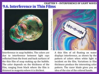
Interference in soap bubbles. The colors are
due to interference between light rays
reflected from the front and back surfaces of
the thin film of soap making up the bubble.
The color depends on the thickness of the
film, ranging from black where the film is
thinnest to magenta where it is thickest.
A thin film of oil floating on water
displays interference, as shown by the
pattern of colors when white light is
incident on the film. Variations in film
thickness produce the interesting color
pattern. The razor blade gives you an
idea of the size of the colored bands.

Newton’s rings
 The interference effect is due to the
combination of ray 1, reflected from
the flat plate, with ray 2, reflected from
the curved surface of the lens.
 Ray 1 undergoes a phase change of
180° upon reflection, whereas ray 2
undergoes no phase change.
→ The dark rings have radii:
Photograph of Newton’s rings
where m: order number
λ: wavelength of the light in free space
R: radius of curvature of the lens
n: refractive index of the film

Application of Newton’s rings
 One important use of Newton’s rings
is in the testing of optical lenses.
 A circular pattern like that pictured in
the upper figure is obtained only
when the lens is ground to a perfectly
symmetric curvature.
 Variations from such symmetry might
produce a pattern like that shown in
the lower figure. These variations
indicate how the lens must be
reground and repolished to remove
imperfections.

Example 9.3
Calculate the minimum thickness of a soap-bubble film that
results in constructive interference in the reflected light if the
film is illuminated with light whose wavelength in free space is
 = 600 nm. The index of refraction of the soap film is 1.33.

Example 9.3

Example 9.4.
Solar cells devices that generate electricity when exposed to
sunlight are often coated with a transparent, thin film of silicon
monoxide (SiO, n = 1.45) to minimize reflective losses from the
surface. Suppose a silicon solar cell (n = 3.5) is coated with a thin
film of silicon monoxide for this purpose. Determine the
minimum film thickness that produces the least reflection at a
wavelength of 550 nm, near the center of the visible spectrum.

Example 9.4.
The left figure shows the path
of the rays in the SiO film that
result in interference in the
reflected light. We can
categorize this as a thin-film
interference problem. To
analyze the problem, note that
the reflected light is a minimum
when rays 1 and 2 in the figure
meet the condition of
destructive interference. In this
situation, both rays undergo a
180° phase change upon
reflection—ray 1 from the upper
SiO surface and ray 2 from the
lower SiO surface.

Example 9.4.
The net change in phase due to
reflection is therefore zero, and the
condition for a reflection minimum
requires a path difference of λn/2,
where λn is the wavelength of the
light in SiO.
→ 2t = λ/2n
where λ is the wavelength in air
and n is the index of refraction of
SiO.
→ The required thickness is

An air wedge is formed between two glass plates separated at
one edge by a very fine wire of circular cross section as shown
in Figure. When the wedge is illuminated from above by 600-nm
light and viewed from above, 30 dark fringes are observed.
Calculate the diameter d of the wire.
Exercise 9.39.

Exercise 9.39.
𝑡 =
𝑚𝜆
2
=
29 × 600 × 10−9
2
= 8.7 × 10−6
𝑚 = 8.7 𝜇𝑚
The diameter of the wire is as the same as the thickness:
d = t = 8.7 µm

The interferometer, invented by American physicist
A. A. Michelson (1852–1931), can be used to measure wavelengths or other
lengths with great precision.
9.7. TheMichelsonInterferometer

DIFFRACTION PATTERNS AND POLARIZATION
CHAPTER 10 (3)
10.1 Introduction to Diffraction
Patterns
10.2 Diffraction Patterns from Narrow
Slits
10.3 Resolution of Single-Slit and
Circular Apertures
10.4 The Diffraction Grating
10.5 Diffraction of X-Rays by Crystals
10.6 Polarization of Light Waves

10.1 Introduction to DiffractionPatterns
CHAPTER 10 – DIFFRACTION PATTERNS AND POLARIZATION
A plane wave of wavelength λ is incident on a barrier in which there is
an opening of diameter d.
When λ << d, the
rays continue in a
straight-line path.
When λ ≈ d, the rays
spread out after
passing through the
opening. This effect is
called diffraction.
When λ >> d, the
opening behaves as a
point source emitting
spherical waves.

 The diffraction phenomenon indicates that
light, once it has passed through a narrow
slit, spreads beyond the narrow path
defined by the slit into regions that would
be in shadow if light traveled in straight
lines.
 Diffraction occurs not only for light waves,
but also for sound waves and water waves.
 The diffraction pattern appears on a
screen when light passes through a narrow
vertical slit. The pattern consists of a broad
central fringe (central maximum), flanked
by a series of narrower, less intense
additional bands (side maxima or
secondary maxima) and a series of
intervening dark bands (minima).

Light from a small source passes by the edge of an opaque
object and continues on to a screen. A diffraction pattern
consisting of bright and dark fringes appears on the screen in
the region above the edge of the object.

 Diffraction pattern created by the illumination of a penny, with the
penny positioned midway between the screen and light source.
 A bright spot occurs at the center, and circular fringes extend
outward from the shadow’s edge.
 The central bright spot can be only explained by using the wave
theory of light, which predicts constructive interference at this
point.
Note the bright
spot at the center

10.2 DiffractionPatternsfrom Narrow Slits
Fraunhofer diffraction pattern Fresnel diffraction pattern
• The light passing through a
narrow opening is modeled as
a slit, and projected onto a
screen.
• The observing screen is far
from the slit, so that the rays
reaching the screen are
approximately parallel. This
can also be achieved
experimentally by using a
converging lens to focus the
parallel rays on a nearby
screen.
• The screen is brought
close to the slit and no
lens is used.
• The Fresnel pattern is
more difficult to analyze
than Fraunhofer
diffraction.

(a) Geometry for
analyzing the Fraunhofer
diffraction pattern of a
single slit, which shows
light entering a single slit
from the left and
diffracting as it propagates
toward a screen (Drawing
not to scale).
(b) Simulation of a single-
slit Fraunhofer diffraction
pattern.
Fraunhofer diffraction pattern

Considering waves leaving the slit as
waves coming from various portions
of the slit:
 Each portion of the slit acts as a
source of light waves.
 Light from one portion of the slit
can interfere with light from
another portion.
→ a diffraction pattern is actually
an interference pattern in which
the different sources of light are
different portions of the single
slit.
Explanation of Fraunhofer diffraction pattern

+ Let’s divide the slit into 𝑛
halves, the path difference
between two adjacent portions
of the single slit is
𝒂
𝒏
𝐬𝐢𝐧𝜽 (𝑎: the width of slit)
+ If 𝑛 is an even number (𝑛 =
2𝑚) and waves from adjacent
portions of the single slit cancel
each other, which is
𝑎
𝑛
sin 𝜃 =
𝜆
2
or
𝐬𝐢𝐧 𝜽 = 𝒎
𝝀
𝒂
𝑚 = ±1, ±2, … ,
we observe dark fringes.
Condition for destructive interference for a single slit

Condition for intensity minima for a single slit:
𝐬𝐢𝐧 𝜽 = 𝒎
𝝀
𝒂
𝑚 = ±1, ±2, ±3, …
Light intensity at a point on the screen:
𝑰 = 𝑰𝒎𝒂𝒙
𝒔𝒊𝒏 𝝅𝒂𝒔𝒊𝒏𝜽/𝝀
𝝅𝒂𝒔𝒊𝒏𝜽/𝝀
𝟐
Condition for destructive interference for a single slit

The diffraction
pattern is produced
when 650-nm light
waves pass through
two 3.0-µm slits
that are 18 mm
apart.
Two-Slit Diffraction Pattern

 Consider not only diffraction patterns due to the individual slits but
also the interference patterns due to the waves coming from different
slits.
 Light intensity at a point on the screen:
𝑰 = 𝑰𝒎𝒂𝒙𝒄𝒐𝒔𝟐
𝝅𝒅𝒔𝒊𝒏𝜽
𝝀
𝒔𝒊𝒏 𝝅𝒂𝒔𝒊𝒏𝜽/𝝀
𝝅𝒂𝒔𝒊𝒏𝜽/𝝀
𝟐
in which the single-slit diffraction pattern (the factor in square
brackets) acting as an “envelope” for a two-slit interference pattern
(the cosine-squared factor)
 The broken blue curve represents the factor in square brackets in the
equation.
 The cosine-squared factor by itself would give a series of peaks all
with the same height as the highest peak of the red-brown curve in
the Figure. Because of the effect of the square-bracket factor,
however, these peaks vary in height.
Two-Slit Diffraction Pattern

Diffraction Patterns from various slits

Exercise 10.6:
Light of wavelength 587.5 nm illuminates a single slit 0.750 mm
in width.
(a) At what distance from the slit should a screen be located if the
first minimum in the diffraction pattern is to be 0.850 mm
from the center of the principal maximum?
(b) What is the width of the central maximum?

Exercise 10.6:

Example 1:
A beam of monochromatic light is incident on a single slit of
width 0.600 mm. A diffraction pattern forms on a wall 1.30 m
beyond the slit. The distance between the positions of zero
intensity on both sides of the central maximum is 2.00 mm.
Calculate the wavelength of the light.

Example 1:

+ If the two sources
which are not coherent
are far enough apart
(Fig. a) to keep their
central maxima from
overlapping → their
images are said to be
resolved.
+ If the sources are close
together (Fig. b), the two
central maxima overlap
→ the images are not
resolved.
Rayleigh’s criterion of resolution
When the central maximum of one image falls on the first minimum
of another image, the images are said to be just resolved.
10.3 ResolutionofSingle-SlitandCircularApertures

The limiting angle of resolution
 for a slit of width 𝑎: 𝜽𝒎𝒊𝒏 =
𝝀
𝒂
 for a circular aperture of diameter 𝐷:
𝜽𝒎 = 𝟏. 𝟐𝟐
𝝀
𝑫
10.3 ResolutionofSingle-SlitandCircularApertures

10.4 TheDiffractionGrating
The diffraction grating, a useful device for analyzing light sources,
consists of a large number of equally spaced parallel slits.
Side view of a diffraction grating. The
slit separation is d, and the path
difference between adjacent slits is d
sin θ

Exercise 10.26
A helium–neon laser ( = 632.8 nm) is used to calibrate a
diffraction grating. If the first-order maximum occurs at 20.5°,
what is the spacing between adjacent grooves in the grating?
Conditionforinterferencemaximaforagrating

Exercise 10.26
1.81 µm

Exercise 10.27
Three discrete spectral lines occur at angles of 10.1°, 13.7°, and
14.8° in the first-order spectrum of a grating spectrometer. (a) If
the grating has 3660 slits/cm, what are the wavelengths of the
light? (b) At what angles are these lines found in the second-
order spectrum?

Exercise 10.27
10.1o
13.7o
30.7o
28.3o
20.5o
10.1o
14.8o

A grating with 250 grooves/mm is used with an incandescent
light source. Assume the visible spectrum to range in wavelength
from 400 nm to 700 nm. In how many orders can one see
(a) the entire visible spectrum,
(b) the short-wavelength region of the visible spectrum.
Exercise 10.33

Exercise 10.33
o
o

Resolving Power of the Diffraction Grating
𝑹 =
𝝀
|𝚫𝝀|
= 𝒎𝑵
• 𝜆 =
𝜆1+𝜆2
2
• Δ𝜆 = 𝜆1 − 𝜆2
In order to distinguish two closely spaced wavelengths 𝜆1 and
𝜆2, the minimum number of illuminated slits must be
𝑵𝐦𝐢𝐧 =
𝑹
𝒎
=
𝟏
𝒎
𝝀
|𝜟𝝀|
• 𝑚: integer (order of maxima)
• 𝑁: the number of illuminated slits
For two nearly equal wavelengths 𝜆1 and 𝜆2 between which a
diffraction grating can just barely distinguish, the resolving
power R of the grating is defined as

Holography: an interesting application of diffraction grating

• The atomic spacing in a solid
(~0.1 nm) → the regular array of
atoms in a crystal could act as a
three-dimensional diffraction
grating for x-rays.
• A collimated beam of
monochromatic x-rays is incident
on a crystal.
• The diffracted beams are very
intense in certain directions
→ constructive interference.
• The diffracted beams (detected
by a photographic film) form an
array of spots known as a Laue
pattern.
10.5 Diffractionof X-RaysbyCrystals
• We can deduce the crystalline structure by analyzing the positions and
intensities of the various spots in the pattern.

Condition for constructive interference (maxima in the reflected beam):

Example 2:
Monochromatic x-rays ( = 0.166 nm) from a nickel target are
incident on a potassium chloride (KCl) crystal surface. The
spacing between planes of atoms in KCl is 0.314 nm. At what
angle (relative to the surface) should the beam be directed for a
second-order maximum to be observed?
o

Example 3:
The first-order diffraction maximum is observed at 12.6° for a crystal
having a spacing between planes of atoms of 0.250 nm.
(a) What wavelength x-ray is used to observe this first-order pattern?
(b) How many orders can be observed for this crystal at this
wavelength?
o

+ An ordinary beam of light
consists of a large number
of waves emitted by the
atoms of the light source.
+ Each atom produces a
wave having some particular
orientation of 𝐸.
10.6 Polarizationof LightWaves
→ The direction of polarization of each individual wave is
defined to be the direction in which 𝐸 is vibrating.
+ All directions of vibration from a wave source are possible.
→ The resultant electromagnetic wave is a superposition of waves
whose 𝐸 vibrate in many different directions.
→ Resultant electromagnetic wave is called an unpolarized wave.

+ Unpolarized light beam:
Figure a (A representation of
an unpolarized light beam
viewed along the direction of
propagation. The transverse
electric field can vibrate in
any direction in the plane of
the page with equal
probability.)
+ Linearly polarized light
beam: Figure b (A linearly
polarized light beam with the
electric field vibrating in the
vertical direction.)

Polarization by Selective Absorption

Polarization by Reflection
+θp: polarizing angle
+n: refraction index
of the reflecting
substance

RELATIVITY
CHAPTER 11
11.1 The Principle of Galilean Relativity
11.2 The Michelson–Morley
Experiment
11.3 Einstein’s Principle of Relativity
11.4 Consequences of the Special
Theory of Relativity
11.5 The Lorentz Transformation Equations
11.6 The Lorentz Velocity Transformation Equations
11.7 Relativistic Linear Momentum and the Relativistic Form of
Newton’s Laws
11.8 Relativistic Energy
11.9 Mass and Energy
11.10 The General Theory of Relativity

3
The Principle of Galilean Relativity
The laws of mechanics must be the same in all inertial frames of
reference.
11.1 ThePrincipleof GalileanRelativity
CHAPTER 11 – RELATIVITY

4
• Consider two inertial frames
S and S’.
• The S’ frame moves with a
constant velocity 𝒗 along the
common 𝒙 and 𝒙′ axes, where
𝒗 is measured relative to S.
• Galilean space–time
transformation equations:
• Galilean velocity
transformation equations:

According to
Galilean relativity,
the speed of light
should not be the
same in all
inertial frames.
Maxwell’s
equations imply
that the speed of
light always has
the fixed value in all
inertial frames.
Speed of light

6
The Michelson–Morley experiment was
repeated at different times of the year
when the ether wind was expected to
change direction and magnitude, but
the results were always the same: no
fringe shift of the magnitude
required was ever observed.
The experiment was designed to
determine the velocity of the Earth
relative to that of the hypothetical ether.
The experimental tool used was the
Michelson interferometer.
11.2 TheMichelson–MorleyExperiment

7
• The negative results of the
Michelson–Morley experiment not
only contradicted the ether
hypothesis but also showed that it
was impossible to measure the
absolute velocity of the Earth with
respect to the ether frame.
• However, Einstein offered a postulate
for his special theory of relativity
that places quite a different
interpretation on these null results.
• In later years, when more was known
about the nature of light, the idea of
an ether that permeates all of space
was abandoned.
11.2 TheMichelson–MorleyExperiment

 The principle of relativity: The laws of physics must be the
same in all inertial reference frames.
 The constancy of the speed of light: The speed of light in
vacuum has the same value, c = 3.00 108 m/s, in all inertial
frames, regardless of the velocity of the observer or the
velocity of the source emitting the light.
Albert Einstein
German-American Physicist (1879–1955)
Einstein, one of the greatest physicists of all
time, was born in Ulm, Germany. In 1905, at age
26, he published four scientific papers that
revolutionized physics. Two of these papers
were concerned with what is now considered
his most important contribution: the special
theory of relativity.
11.3 Einstein’sPrincipleof Relativity

Simultaneity and the Relativity of Time
11.4. Consequencesof theSpecialTheoryof Relativity
Two events that are simultaneous in one reference frame are in
general not simultaneous in a second frame moving relative to
the first. That is, simultaneity is not an absolute concept but
rather one that depends on the state of motion of the observer.

Simultaneity and the Relativity of Time
• Einstein’s thought experiment
demonstrates that two
observers can disagree on the
simultaneity of two events.
• This disagreement depends on
the transit time of light to the
observers.
• In relativistic analyses of high-
speed situations, relativity
shows that simultaneity is
relative even when the transit
time is subtracted out.

11
Time Dilation

12
where Δt: the time interval measured by observer O in second frame
𝚫𝒕𝒑: Proper time interval (the proper time interval is the
time interval between two events measured by an
observer who sees the events occur at the same point in
space.)
v: moving speed of the second frame respect to the first
frame
γ: proportional factor
Time Dilation

13
The time interval measured in any
other reference frame is always
longer than the proper time. This
expansion is called time dilation.
Time Dilation

14
Example 1
A deep-space vehicle moves away from the Earth with a speed
of 0.800c. An astronaut on the vehicle measures a time interval
of 3.00 s to rotate her body through 1.00 rev as she floats in the
vehicle. What time interval is required for this rotation
according to an observer on the Earth?
Time Dilation

15
Exercise 11.6
At what speed does a clock move if it is measured to run at a rate
that is half the rate of a clock at rest with respect to an observer?
Time Dilation

16
The Twin Paradox
The twin paradox.
Speedo takes a
journey to a star
20 light-years
away and returns
to the Earth.

Length Contraction
If an object has a proper length 𝐿𝑝, its length 𝐿 when it moves
with speed 𝒗 in a direction parallel to its length is measured
to be shorter.
where L: length of an object when it is measured by an observer
moving with speed v in a direction parallel to its length
𝑳𝒑: Proper length (The length of an object measured by an
observer at rest with respect to the object)

18
Length Contraction
A meter stick measured by an
observer in a frame attached
to the stick (that is, both have
the same velocity) has its
proper length Lp.
The stick measured by an
observer in a frame in which the
stick has a velocity v relative to
the frame is measured to be
shorter than its proper length Lp.

19
Example 2
A star is 5.00 ly from the Earth. At what speed must a spacecraft
travel on its journey to the star such that the Earth–star distance
measured in the frame of the spacecraft is 2.00 ly?
Length Contraction

20
Example 11.5
An astronaut takes a trip to Sirius, which is located a distance of 8
light-years from the Earth. The astronaut measures the time of
the one-way journey to be 6 years. If the spaceship moves at a
constant speed of 0.8c, how can the 8-ly distance be reconciled
with the 6-year trip time measured by the astronaut?
Length Contraction

21
Length Contraction
Solution:
The distance of 8 ly represents the proper length from the Earth
to Sirius measured by an observer seeing both objects nearly at
rest. The astronaut sees Sirius approaching her at 0.8c but also
sees the distance contracted to

22
 One important consequence of time dilation is the relativistic
Doppler effect (the shift in frequency found for light emitted by
atoms in motion as opposed to light emitted by atoms at rest).
 The frequency fobs measured by the observer is
The relativistic Doppler effect
Where fsource: frequency of the source measured in its rest frame
v: relative speed between the light source and the observer
v > 0 when a light source and an observer approach (moving
toward) each other
v < 0 when the source and the observer recede (moving away)
from each other

23
• Consider two inertial frames
S and S’.
• The S’ frame moves with a
constant velocity 𝑣 along the
common 𝑥 and 𝑥′ axes,
where 𝑣 is measured relative
to S.
Lorentz transformation for S → S’
𝒙′
= 𝜸 𝒙 − 𝒗𝒕 , 𝒚′
= 𝒚, 𝒛′
= 𝒛, 𝒕′
= 𝜸 𝒕 −
𝒗
𝒄𝟐
𝒙
11.5. TheLorentz TransformationEquations
Lorentz transformation for S’ → S
𝒙 = 𝜸 𝒙′ + 𝒗𝒕′ , 𝒚 = 𝒚′, 𝒛 = 𝒛′, 𝒕 = 𝜸 𝒕′ +
𝒗
𝒄𝟐
𝒙′

24
• When v << c, Lorentz transformation equations should reduce to the
Galilean equations.
11.5. TheLorentz TransformationEquations

11.6. TheLorentz VelocityTransformationEquations
Lorentz velocity transformation for S → S’
𝒖𝒙
′ =
𝒖𝒙 − 𝒗
𝟏 −
𝒗
𝒄𝟐 𝒖𝒙
, 𝒖𝒚
′ =
𝒖𝒚
𝜸 𝟏 −
𝒗
𝒄𝟐 𝒖𝒙
, 𝒖𝒛
′ =
𝒖𝒛
𝜸 𝟏 −
𝒗
𝒄𝟐 𝒖𝒙
Lorentz velocity transformation for S’ → S
𝒖𝒙 =
𝒖𝒙
′
+ 𝒗
𝟏 +
𝒗
𝒄𝟐 𝒖𝒙
′
, 𝒖𝒚 =
𝒖𝒚
′
𝜸 𝟏 +
𝒗
𝒄𝟐 𝒖𝒙
′
, 𝒖𝒛 =
𝒖𝒛
′
𝜸 𝟏 +
𝒗
𝒄𝟐 𝒖𝒙
′
• When v << c: 𝒖𝒙
′
≈ 𝒖𝒙 − 𝒗
• When 𝒖𝒙 = 𝒄: 𝒖𝒙
′ = 𝒄
→ a speed measured as c by an observer in S is also measured as c
by an observer in S’—independent of the relative motion of S
and S’.
→ the speed of light is the ultimate speed.

Definition of relativistic linear momentum
𝑚: mass of the particle
𝑢: velocity of the particle
→ The relativistic force 𝐹 acting on a particle whose linear
momentum is 𝑝:
𝛾 =
1
1 −
𝑢2
𝑐2
11.7. RelativisticLinearMomentumandthe
RelativisticForm of Newton’sLaws

27
Example 11.10
An electron, which has a mass of 9.1110-31 kg, moves with a
speed of 0.750c. Find the magnitude of its relativistic momentum
and compare this value with the momentum calculated from the
classical expression.

28
Example 11.10

 Relativistic kinetic energy
 Rest energy
 Total energy of
a relativistic particle
 Energy–momentum relationship for a relativistic particle
11.8. RelativisticEnergy

30
Example 11.12
(A)Find the rest energy of a proton in units of electron volts.
(B)If the total energy of a proton is three times its rest energy,
what is the speed of the proton?
(C) Determine the kinetic energy of the proton in units of
electron volts.
(D)What is the proton’s momentum?

31
Example 11.12

32
Example 11.12

33
Example 11.12

34
Example 11.12

35
Example 11.13
11.9 MassandEnergy

36
Example 11.13
11.9 MassandEnergy

37
Example 11.13
11.9 MassandEnergy

PHYSICS 2 ELECTRICITY MAGNETISM OPTICS AND MODERN PHYSICS.pdf

More Related Content

What's hot (20)

Similar to PHYSICS 2 ELECTRICITY MAGNETISM OPTICS AND MODERN PHYSICS.pdf (20)

More from Nguyen Thanh Tu Collection (20)

Recently uploaded (20)

PHYSICS 2 ELECTRICITY MAGNETISM OPTICS AND MODERN PHYSICS.pdf