Probability based learning (in book: Machine learning for predictve data analytics)
Download as PPTX, PDF1 like1,998 views

The document discusses probability-based learning, focusing on Bayes' theorem fundamentals, which include conditional independence, Bayesian networks, and various prediction models like the naïve Bayes model. It explains key concepts such as prior and posterior probabilities, as well as techniques for smoothing and handling continuous features. Numerous examples illustrate the application of these concepts, with an emphasis on Bayesian prediction and building Bayesian networks.


![With P(t=l): the prior probability of target feature t taking the level l
P(q[1],…,q[m]): joint probability of descriptive feature
P(q[1],…,q[m] | t=l): the conditional probability
Example 1:
Table 6.1
What is probability a person has MENINGTIS when he/she has HEADACHE=true, FEVER=false,
VOMITING=true?
=> P(m | h, -f, v)
Bayesian prediction
P(t=l | q[1],…,q[m]) =
𝑃 𝑞 1 ,…,𝑞 𝑚 𝑡=𝑙)𝑃(𝑡=𝑙)
𝑃(𝑞 1 ,…,𝑞 𝑚 )
6](https://image.slidesharecdn.com/probability-basedlearning-160820122420/85/Probability-based-learning-in-book-Machine-learning-for-predictve-data-analytics-6-320.jpg)
![P(m | h, -f, v) =
𝑃 ℎ,−𝑓,𝑣 𝑚)𝑃(𝑚)
𝑃(ℎ,−ℎ,𝑣)
P(m) =
|{𝐼𝐷5,𝐼𝐷8,𝐼𝐷10}|
|{𝐼𝐷1,𝐼𝐷2,𝐼𝐷3,𝐼𝐷4,𝐼𝐷5,𝐼𝐷6,𝐼𝐷7,𝐼𝐷8,𝐼𝐷9,𝐼𝐷10}|
= 0.3
P(h,-f,v) =
|{𝐼𝐷3,𝐼𝐷4,𝐼𝐷6,𝐼𝐷7,𝐼𝐷8,𝐼𝐷10}|
|{𝐼𝐷1,𝐼𝐷2,𝐼𝐷3,𝐼𝐷4,𝐼𝐷5,𝐼𝐷6,𝐼𝐷7,𝐼𝐷8,𝐼𝐷9,𝐼𝐷10}|
= 0.6
P(h, -f, v | m) = P(h|m) P(-f | h,m) P(v | -f, h, m)
=
|{𝐼𝐷8,𝐼𝐷10}|
|{𝐼𝐷5,𝐼𝐷8,𝐼𝐷10}|
x
|{𝐼𝐷8,𝐼𝐷10}|
|{𝐼𝐷8,𝐼𝐷10}|
x
|{𝐼𝐷8,𝐼𝐷10}|
|{𝐼𝐷8,𝐼𝐷10}|
=
2
3
x
2
2
x
2
2
= 0.66
P(m | h, -f, v) = (0.66*0.3) / 0.6 = 0.33
P(-m | h, -f, v) =
𝑃 ℎ,−𝑓,𝑣 −𝑚)𝑃(−𝑚)
𝑃(ℎ,−ℎ,𝑣)
=
𝑃 ℎ −𝑚)𝑃(−𝑓 ℎ,−𝑚 𝑃 𝑣 −𝑓,ℎ,−𝑚)𝑃(−𝑚)
𝑃(ℎ,−ℎ,𝑣)
= 0.667
Bayesian prediction
P(t=l | q[1],…,q[m]) =
𝑃 𝑞 1 ,…,𝑞 𝑚 𝑡=𝑙)𝑃(𝑡=𝑙)
𝑃(𝑞 1 ,…,𝑞 𝑚 )
7](https://image.slidesharecdn.com/probability-basedlearning-160820122420/85/Probability-based-learning-in-book-Machine-learning-for-predictve-data-analytics-7-320.jpg)
![Bayesian prediction
Maximum a posterior predction:
M (q) = arg max P(t=l | q[1],…,q[m])
= arg max l ∈ 𝑙𝑒𝑣𝑒𝑙𝑠( 𝑡)
𝑃 𝑞 1 , … , 𝑞 𝑚 𝑡 = 𝑙)𝑃(𝑡 = 𝑙)
𝑃(𝑞 1 , … , 𝑞 𝑚 )
Bayesian MAP prediction model:
M (q) = arg max P(t=l | q[1],…,q[m])
= arg max l ∈ 𝑙𝑒𝑣𝑒𝑙𝑠( 𝑡)
𝑃 𝑞 1 , … , 𝑞 𝑚 𝑡 = 𝑙)𝑃(𝑡 = 𝑙)
8](https://image.slidesharecdn.com/probability-basedlearning-160820122420/85/Probability-based-learning-in-book-Machine-learning-for-predictve-data-analytics-8-320.jpg)
![Example 2:
Table 6.1
What is probability a person has MENINGTIS when he/she has HEADACHE=true, FEVER=true,
VOMITING=false?
P(m | h, f, -v) =
𝑃 ℎ 𝑚 𝑃 𝑓 ℎ, 𝑚 𝑃 −𝑣 𝑓, ℎ, 𝑚 𝑃(𝑚)
𝑃(ℎ,𝑓,−𝑣)
=
0.66 ∗ 0 ∗0 ∗0.3
0.1
= 0.0
P(-m| h, f, -v) = 1.0 – 0.0 = 1.0
Overfit data
Bayesian prediction
P(t=l | q[1],…,q[m]) =
𝑃 𝑞 1 ,…,𝑞 𝑚 𝑡=𝑙)𝑃(𝑡=𝑙)
𝑃(𝑞 1 ,…,𝑞 𝑚 )
9](https://image.slidesharecdn.com/probability-basedlearning-160820122420/85/Probability-based-learning-in-book-Machine-learning-for-predictve-data-analytics-9-320.jpg)
![Conditional independence
when X and Y (independence) share the same cause Z.
P(X | Y, Z) = P(X | Z)
P(X, Y | Z) = P(X | Z)*P(Y | Z)
Chain rule:
P(q[1],…,q[m] | t=l) = P(q[1] | t=l)*P(q[2] | t=l)*…*P(q[m] | t=l)
= Π P(q[i] | t=l)
P(t=l | q[1],…,q[m]) =
Π P(q[i] | t=l) ∗ P(t=l)
𝑃(𝑞 1 ,…,𝑞 𝑚 )
= Joint probability:
P(H,F,V,M) = P(M) * P(H|M) * P(F|M) * P(V|M)
Conditional independence and Factorization10
If X and Y are independent, then:
P(X|Y) = P(X)
P(X, Y) = P(X) P(Y)](https://image.slidesharecdn.com/probability-basedlearning-160820122420/85/Probability-based-learning-in-book-Machine-learning-for-predictve-data-analytics-10-320.jpg)

![Example
Table 6.2
Naïve Bayes Model12
MAP (Maximum a posterior):
M(q) = arg maxl ∈ levels(t) ((Πi P(q[i] | t=l) * P(t=l))](https://image.slidesharecdn.com/probability-basedlearning-160820122420/85/Probability-based-learning-in-book-Machine-learning-for-predictve-data-analytics-12-320.jpg)


![P(t |d[1], …, d[n]) = P(t) * ∏ P(d[j] | t)
Naïve Bayes Classifier18
Target
Descriptive
feature 1
Descriptive
feature 2
Descriptive
feature n](https://image.slidesharecdn.com/probability-basedlearning-160820122420/85/Probability-based-learning-in-book-Machine-learning-for-predictve-data-analytics-18-320.jpg)


Probability based learning (in book: Machine learning for predictve data analytics)
- 1. Summary: Probability-based Learning (from book: Machine learning for predictve data analytics) Duyen Do 1
- 2. NỘI DUNG Bayes’ Theorem Fundamentals Bayes Prediction Standard Approach: The Naïve Bayes Model Conditional Independence and Factorization Smoothing Extensions and Variations Continuous Features Bayesian Network Summary Q&A Probability basic 2
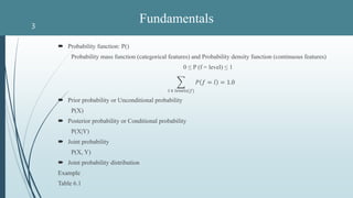
- 3. Probability function: P() Probability mass function (categorical features) and Probability density function (continuous features) 0 ≤ P (f = level) ≤ 1 𝑙 ∈ 𝑙𝑒𝑣𝑒𝑙𝑠(𝑓) 𝑃 𝑓 = 𝑙 = 1.0 Prior probability or Unconditional probability P(X) Posterior probability or Conditional probability P(X|Y) Joint probability P(X, Y) Joint probability distribution Example Table 6.1 Fundamentals3
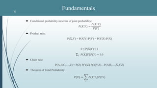
- 4. Conditional probability in terms of joint probability: 𝑃(𝑋|𝑌) = 𝑃(𝑋, 𝑌) 𝑃(𝑌) Product rule: P(X,Y) = P(X|Y) P(Y) = P(Y|X) P(X) 0 ≤ P(X|Y) ≤ 1 𝑖 𝑃 𝑋𝑖 𝑌 𝑃(𝑌) = 1.0 Chain rule: P(A,B,C,…,Z) = P(Z) P(Y|Z) P(X|Y,Z)…P(A|B,…,X,Y,Z) Theorem of Total Probability: 𝑃(𝑋) = 𝑖 𝑃 𝑋 𝑌𝑖 𝑃(𝑌𝑖) Fundamentals4
- 5. Fundamentals: Bayes’s Theorem P(X|Y) = 𝑃(𝑌|𝑋)𝑃(𝑋) 𝑃(𝑌) A doctor inform a patient both bad news and good news: - Bad news: 99% has a serious desease - Good news: the desease is rarely and only 1 in 10,000 people What is actually probability that patient has the desease? Using Bayes’Theorem: 𝑃 𝑑 𝑡 = 𝑃 𝑡 𝑑 𝑃 𝑑 𝑃 𝑡 P(t) = P(t|d)P(d) + P(t|-d)P(-d) = (0.99 * 0.0001) + (0.01 * 0.9999) = 0.0101 P(d|t) = 0.99 ∗0.0001 0.0101 = 0.0098 5
- 6. With P(t=l): the prior probability of target feature t taking the level l P(q[1],…,q[m]): joint probability of descriptive feature P(q[1],…,q[m] | t=l): the conditional probability Example 1: Table 6.1 What is probability a person has MENINGTIS when he/she has HEADACHE=true, FEVER=false, VOMITING=true? => P(m | h, -f, v) Bayesian prediction P(t=l | q[1],…,q[m]) = 𝑃 𝑞 1 ,…,𝑞 𝑚 𝑡=𝑙)𝑃(𝑡=𝑙) 𝑃(𝑞 1 ,…,𝑞 𝑚 ) 6
- 7. P(m | h, -f, v) = 𝑃 ℎ,−𝑓,𝑣 𝑚)𝑃(𝑚) 𝑃(ℎ,−ℎ,𝑣) P(m) = |{𝐼𝐷5,𝐼𝐷8,𝐼𝐷10}| |{𝐼𝐷1,𝐼𝐷2,𝐼𝐷3,𝐼𝐷4,𝐼𝐷5,𝐼𝐷6,𝐼𝐷7,𝐼𝐷8,𝐼𝐷9,𝐼𝐷10}| = 0.3 P(h,-f,v) = |{𝐼𝐷3,𝐼𝐷4,𝐼𝐷6,𝐼𝐷7,𝐼𝐷8,𝐼𝐷10}| |{𝐼𝐷1,𝐼𝐷2,𝐼𝐷3,𝐼𝐷4,𝐼𝐷5,𝐼𝐷6,𝐼𝐷7,𝐼𝐷8,𝐼𝐷9,𝐼𝐷10}| = 0.6 P(h, -f, v | m) = P(h|m) P(-f | h,m) P(v | -f, h, m) = |{𝐼𝐷8,𝐼𝐷10}| |{𝐼𝐷5,𝐼𝐷8,𝐼𝐷10}| x |{𝐼𝐷8,𝐼𝐷10}| |{𝐼𝐷8,𝐼𝐷10}| x |{𝐼𝐷8,𝐼𝐷10}| |{𝐼𝐷8,𝐼𝐷10}| = 2 3 x 2 2 x 2 2 = 0.66 P(m | h, -f, v) = (0.66*0.3) / 0.6 = 0.33 P(-m | h, -f, v) = 𝑃 ℎ,−𝑓,𝑣 −𝑚)𝑃(−𝑚) 𝑃(ℎ,−ℎ,𝑣) = 𝑃 ℎ −𝑚)𝑃(−𝑓 ℎ,−𝑚 𝑃 𝑣 −𝑓,ℎ,−𝑚)𝑃(−𝑚) 𝑃(ℎ,−ℎ,𝑣) = 0.667 Bayesian prediction P(t=l | q[1],…,q[m]) = 𝑃 𝑞 1 ,…,𝑞 𝑚 𝑡=𝑙)𝑃(𝑡=𝑙) 𝑃(𝑞 1 ,…,𝑞 𝑚 ) 7
- 8. Bayesian prediction Maximum a posterior predction: M (q) = arg max P(t=l | q[1],…,q[m]) = arg max l ∈ 𝑙𝑒𝑣𝑒𝑙𝑠( 𝑡) 𝑃 𝑞 1 , … , 𝑞 𝑚 𝑡 = 𝑙)𝑃(𝑡 = 𝑙) 𝑃(𝑞 1 , … , 𝑞 𝑚 ) Bayesian MAP prediction model: M (q) = arg max P(t=l | q[1],…,q[m]) = arg max l ∈ 𝑙𝑒𝑣𝑒𝑙𝑠( 𝑡) 𝑃 𝑞 1 , … , 𝑞 𝑚 𝑡 = 𝑙)𝑃(𝑡 = 𝑙) 8
- 9. Example 2: Table 6.1 What is probability a person has MENINGTIS when he/she has HEADACHE=true, FEVER=true, VOMITING=false? P(m | h, f, -v) = 𝑃 ℎ 𝑚 𝑃 𝑓 ℎ, 𝑚 𝑃 −𝑣 𝑓, ℎ, 𝑚 𝑃(𝑚) 𝑃(ℎ,𝑓,−𝑣) = 0.66 ∗ 0 ∗0 ∗0.3 0.1 = 0.0 P(-m| h, f, -v) = 1.0 – 0.0 = 1.0 Overfit data Bayesian prediction P(t=l | q[1],…,q[m]) = 𝑃 𝑞 1 ,…,𝑞 𝑚 𝑡=𝑙)𝑃(𝑡=𝑙) 𝑃(𝑞 1 ,…,𝑞 𝑚 ) 9
- 10. Conditional independence when X and Y (independence) share the same cause Z. P(X | Y, Z) = P(X | Z) P(X, Y | Z) = P(X | Z)*P(Y | Z) Chain rule: P(q[1],…,q[m] | t=l) = P(q[1] | t=l)*P(q[2] | t=l)*…*P(q[m] | t=l) = Π P(q[i] | t=l) P(t=l | q[1],…,q[m]) = Π P(q[i] | t=l) ∗ P(t=l) 𝑃(𝑞 1 ,…,𝑞 𝑚 ) = Joint probability: P(H,F,V,M) = P(M) * P(H|M) * P(F|M) * P(V|M) Conditional independence and Factorization10 If X and Y are independent, then: P(X|Y) = P(X) P(X, Y) = P(X) P(Y)
- 11. Example 2: Table 6.1 What is probability a person has MENINGTIS when he/she has HEADACHE=true, FEVER=true, VOMITING=false? P(m | h, f, -v) = P(h |m) ∗ P(f | m) ∗ P(−v | m) ∗ P(m) 𝑃(ℎ,𝑓,−𝑣) = P(h |m) ∗ P(f | m) ∗ P(−v | m) ∗ P(m) Σ𝑖 𝑃 ℎ 𝑀𝑖 ∗𝑃 𝑓 𝑀𝑖 ∗𝑃 −𝑣 𝑀𝑖 ∗𝑃(𝑀𝑖) = 0.1948 P(-m | h, f, -v) = 0.8052 Conditional independence and Factorization11 If X and Y are independent, then: P(X|Y) = P(X) P(X, Y) = P(X) P(Y)
- 12. Example Table 6.2 Naïve Bayes Model12 MAP (Maximum a posterior): M(q) = arg maxl ∈ levels(t) ((Πi P(q[i] | t=l) * P(t=l))
- 13. Example Table 6.2 CREDIT HISTORY = paid, GUANRANTOR/COAPPLICANT = guarantor, ACCOMMODATION = free? Extensions and Variations: Smoothing13 Laplace smoothing: 𝑃 𝑓 = 𝑙 𝑡) = 𝑐𝑜𝑢𝑛𝑡 𝑓 = 𝑙 𝑡) + 𝑘 𝑐𝑜𝑢𝑛𝑡 𝑓 𝑡) + (𝑘 ∗ 𝐷𝑜𝑚𝑎𝑖𝑛 𝑓 )
- 14. Transform continuous feature to categorical feature with: Equal-width binning Equal-frequency binning Example Table 6.11 Extensions and Variations: Continuous feature - Binning14
- 15. A Bayesian network, Bayes network, Bayes(ian) model or probabilistic directed acyclic graphical model is a probabilistic graphical model that represents a structural relationship - a set of random variables and their conditional dependencies - via a directed acyclic graph (DAG) P(A,B) = P(B|A) * P(A) Ex1: P(a, -b) = P(-b|a) * P(a) = 0.7 * 0.4 = 0.28 The probability of an event x1,…,xn P(x1,…,xn) = ∏ P(xi | Parents(xi)) Bayesian Network15 A B P(A=T) P(A=F) 0.4 0.6 A P(B=T | A) P(B=F | A) T 0.3 0.7 F 0.4 0.6
- 16. Ex2: P (a, -b, -c, d) = P(-b|a,-c) * P(-c|d) * P(a) * P(d) = 0.5 * 0.8 * 0.4 * 0.4 = 0.064 Bayesian Network16 A B C D P(D=T) 0.4 P(A=T) 0.4 D P(C=T|D) T 0.2 F 0.5 A C P(B=T|A,C) T T 0.2 T F 0.5 F T 0.4 F F 0.3
- 17. The conditional probability of node xi with n nodes P(xi | x1,…, xi-1, xi+1,…,xn) = P(xi | Parents(xi) ∏ P(xj | Parents(xj)) with j ∈ Children(xi) Ex2: P(c | -a, b, d) = P(c | d) * P(b | -a, c) = 0.2 * 0.4 = 0.08 Bayesian Network17 A B C D P(D=T) 0.4 P(A=T) 0.4 D P(C=T|D) T 0.2 F 0.5 A C P(B=T|A,C) T T 0.2 T F 0.5 F T 0.4 F F 0.3
- 18. P(t |d[1], …, d[n]) = P(t) * ∏ P(d[j] | t) Naïve Bayes Classifier18 Target Descriptive feature 1 Descriptive feature 2 Descriptive feature n
- 19. P(A, B, C) = P(C | A, B) * P(B |A) * P(A) P(A, B, C) = P(A| C, B) * P(B |C) * P(C) Building Bayesian Network19 B C A A C B P(A=T) 0.6 P(C=T) 0.2 A P(B=T|A) T 0.333 F 0.5 C P(B=T|C) T 0.5 F 0.375 A B P(C|A,B) T T 0.25 T F 0.125 F T 0.25 F F 0.25 C B P(A|B,C) T T 0.5 T F 0.5 F T 0.5 F F 0.7
- 20. Building Bayesian Network20 Hybrid approach: 1. Given the topology of the network 2. Induce the CPT What is the best topology structure to give the algorithm as input? Causal graphs Example Table 6.18
- 21. Building Bayesian Network21 A potential causal theory: The more equal in a society, the higher the investment that society will make in health and education, and this in turn result in a lower of corruption SY LE P(CPI|SY, LE) L L 1.0 L H 0 H L 1.0 H H 1.0 CPI GC SC LE GC P(SY=L|GC) L 0.2 H 0.8 GC P(LE=L|GC) L 0.2 H 0.8 B P(GC=L) T 0.5
- 22. Using Bayesian Network make predictions22 M (q) = arg max l ∈ levels(t) BayesianNetwork(t=l,q) Making prediction with missing descriptive feature values: GC = high, SC = high =>? Example Table 6.18