Python_ppt for basics of python in details
Download as PPTX, PDF0 likes155 views

The document provides a comprehensive overview of Python, covering topics from basic syntax and data types to advanced features such as functions, libraries, and control structures. It discusses the history of Python, its applications in various domains, and installation instructions for different operating systems. Additionally, it outlines key concepts including variables, operators, data type conversions, and conditional statements.


![SET ENVIRONMENT VARIABLE
1. Select “path” variable in system variables
2. Click on edit button
3. Add following path in the path variable
C:Users[Your_Current_User_Name]AppData
LocalProgramsPythonPython36;
Then click on ok Button.
Now open command prompt and type python
If python shall is running then environment variable
is set properly.](https://image.slidesharecdn.com/pythonppt-241219160842-b89b61db/85/Python_ppt-for-basics-of-python-in-details-19-320.jpg)


![CONTINUE….
Example:
fruits = [‘Grapes', 'apple', ‘pineapple']
for fruit in fruits:
print( 'Current fruit :', fruit ,’n’ )
Output:
Current fruit : Grapes
Current fruit : apple
Current fruit : pineapple](https://image.slidesharecdn.com/pythonppt-241219160842-b89b61db/85/Python_ppt-for-basics-of-python-in-details-61-320.jpg)


![ACCESSING VALUES IN STRINGS
To access substrings, use the square brackets for slicing along
with the index or indices to obtain your substring.
Ex.
string1 = “python is awesome”
string2 = “yes it is"
print (string2[0] )
Output:
‘py’
print (string2[1:5])
Output:
ythoes i](https://image.slidesharecdn.com/pythonppt-241219160842-b89b61db/85/Python_ppt-for-basics-of-python-in-details-80-320.jpg)
![UPDATE STRINGS
Ex
var1 = ‘hi my name is xyz‘
print(var1[:6] + ‘mukul’)
Output:
‘hi my mukul’
Do not Update a single a char in string like this;
var1[14]=‘a’
Print(var1)
Output:
‘Error’](https://image.slidesharecdn.com/pythonppt-241219160842-b89b61db/85/Python_ppt-for-basics-of-python-in-details-81-320.jpg)


![STRING SPECIAL OPERATORS
Operator Description
+ For Concatenation
* Repetition
[] Slice
[ : ] Range Slice
in Membership
not in Membership
r/R Raw String](https://image.slidesharecdn.com/pythonppt-241219160842-b89b61db/85/Python_ppt-for-basics-of-python-in-details-86-320.jpg)
![ITERATE STRING WITH FOR LOOP
str1=“My Name”
for j in str1:
print(j,”n”)
Output:
M
Y
[white space]
N
a
m
e](https://image.slidesharecdn.com/pythonppt-241219160842-b89b61db/85/Python_ppt-for-basics-of-python-in-details-87-320.jpg)
![PYTHON LISTS
The list can be written as a collection of
comma-separated values (items) between
square brackets. Values can be any type of.
Eg.
list1 = ['physics', 'chemistry', 1997, 2000];
list2 = [1, 2, 3, 4, 5 ];
list3 = ["a", "b", "c", "d"]](https://image.slidesharecdn.com/pythonppt-241219160842-b89b61db/85/Python_ppt-for-basics-of-python-in-details-88-320.jpg)
![ACCESSING VALUES IN LISTS
Ex.
list1 = ['physics', 'chemistry', 1997, 2000];
list2 = [1, 2, 3, 4, 5, 6, 7 ];
#printing Single value in list :-
Print(list1[0])
Output:
‘physics’
Ex.
#print set of continuous values in list
print (list2[1:5])
Output:
1,2,3,4](https://image.slidesharecdn.com/pythonppt-241219160842-b89b61db/85/Python_ppt-for-basics-of-python-in-details-89-320.jpg)
![UPDATING LISTS
Ex.
list = ['physics', 'chemistry', 1997, 2000];
list[2]=1999
Print(list)
Output:
['physics', 'chemistry', 1999, 2000]
Ex.
list[2:3]=2,3
print (list)
Output:
['physics', 'chemistry', 2, 3]](https://image.slidesharecdn.com/pythonppt-241219160842-b89b61db/85/Python_ppt-for-basics-of-python-in-details-90-320.jpg)
![APPEND ELEMENT IN LIST
Ex.
List1=[1,2,3]
print(List1)
Output:
[1,2,3]
Ex.
List1.append(2)
Print(list)
Output:
[1,2,3,2]](https://image.slidesharecdn.com/pythonppt-241219160842-b89b61db/85/Python_ppt-for-basics-of-python-in-details-91-320.jpg)
![DELETE LIST ELEMENTS
Ex.
list1 = [‘MUKUL', ‘KIRTI', 1989,2000];
del list1[3];
Print( list1)
Output:
[‘MUKUL', ‘KIRTI', 1989]
But if we execute
del list1
Then whole list will be deleted](https://image.slidesharecdn.com/pythonppt-241219160842-b89b61db/85/Python_ppt-for-basics-of-python-in-details-92-320.jpg)


![ACCESSING VALUES IN TUPLES
tup1 = (‘abc', “xyz”, 123, 1.2);
tup2 = (1, 2, 3, 4, 5, 6, 7 );
#printing Single value in tuple :-
print ("tup1[0]: “,tup1[0]);
Output:
(‘abc’)
# print set of continuous values(tuple slicing) in tuple:
print("tup2[1:5]: ", tup2[1:5]);
Output:
(2,3,4,5)](https://image.slidesharecdn.com/pythonppt-241219160842-b89b61db/85/Python_ppt-for-basics-of-python-in-details-96-320.jpg)
![UPDATING TUPLES
Tuples are immutable which means you cannot
update or change the values of tuple elements.
tup1 = (12, 34.56);
tup1[0] = 100;
Output:
TypeError: 'tuple' object does not support item
assignment](https://image.slidesharecdn.com/pythonppt-241219160842-b89b61db/85/Python_ppt-for-basics-of-python-in-details-97-320.jpg)

![DELETE TUPLE ELEMENTS
Because tuple is immutable so element of tuple can not be deleted
Only whole tuple can be deleted.
Ex.
Tuple1=(1,2,3)
del Tuple1[0]
Output:
“Error”
Ex.
del Tuple1 # now Tuple 1 is deleted
Print(Tuple1)
Output:
NameError: variable name tuple1 not defined](https://image.slidesharecdn.com/pythonppt-241219160842-b89b61db/85/Python_ppt-for-basics-of-python-in-details-99-320.jpg)


![ACCESSING VALUES IN DICTIONARY
Ex.
dict1 = {‘2': ‘4', ‘3':’9’, ‘4':‘16'}
print( dict1[‘2'] )
print ( dict1[‘3'] )
Output:
‘4’
‘9’
Note: Dictionary Slicing is not possible
Means we an not write:
dict1[1:3]
Output:
‘Error’](https://image.slidesharecdn.com/pythonppt-241219160842-b89b61db/85/Python_ppt-for-basics-of-python-in-details-103-320.jpg)
![UPDATING DICTIONARY
dict1 = {‘1': ‘1', ‘2': 4, ‘3': ‘9'}
dict1[‘1'] = “11";
print(dict1)
Output:
{‘1': ‘11', ‘2': 4, ‘3': ‘9'}
dict1[‘2’]=‘44’
Print(dict1)
Output:
{‘1': ‘11', ‘2': ’44’, ‘3': ‘9'}](https://image.slidesharecdn.com/pythonppt-241219160842-b89b61db/85/Python_ppt-for-basics-of-python-in-details-104-320.jpg)
![ADDING ELEMENT IN DECTIONARY
Ex.
dict1 = {‘1': ‘1', ‘2': 4, ‘3': ‘9'}
dict1[‘4’]=‘16’
print(dict1)
Output:
{‘1': ‘1’,‘2': 4,‘3': ‘9‘,’4’:’16’}
Ex.
dict1[‘5’]=‘25’
print(dict1)
Output:
{‘1’:’1’,’2’:’4’,’3’:’9’,’4’:’16’,’5’:’25’}](https://image.slidesharecdn.com/pythonppt-241219160842-b89b61db/85/Python_ppt-for-basics-of-python-in-details-105-320.jpg)
![DELETE DICTIONARY ELEMENTS
1. del dict[‘Key_Name']; # remove entry with
key ‘Key_Name‘
2. dict.clear(); # delete all entries in dict
3. del dict ; # delete entire dictionary](https://image.slidesharecdn.com/pythonppt-241219160842-b89b61db/85/Python_ppt-for-basics-of-python-in-details-106-320.jpg)
![ Ex.
dict1 = {‘1': ‘1', ‘2': 4, ‘3': ‘9'}
del dict1[‘2’]
print(dict1)
Output:
{‘1': ‘1', ‘3': ‘9'}
dict1.clear();
print(dict1)
Output:
{}
del dict1
print(dict1)
Output:
“NameError: name 'i' is not defined”](https://image.slidesharecdn.com/pythonppt-241219160842-b89b61db/85/Python_ppt-for-basics-of-python-in-details-107-320.jpg)


![FUNCTION IN PYTHON
A function is a block of code which is run only when, it is called.
Creating or defining a Function;
def functionname( parameters ):
[expression]
Ex.
def printme(str):
print(str)
printme(“hi”)
Output:
‘hi’](https://image.slidesharecdn.com/pythonppt-241219160842-b89b61db/85/Python_ppt-for-basics-of-python-in-details-110-320.jpg)


![VARIABLE-LENGTH ARGUMENTS
You may need to process a function for more
arguments than you specified while defining the
function. These arguments are called variable-
lengtharguments and are not named in the function
definition, unlike required and default arguments.
Syntax:
def function_name(formal_args,*var_args_tuple ):
code
return [expression]](https://image.slidesharecdn.com/pythonppt-241219160842-b89b61db/85/Python_ppt-for-basics-of-python-in-details-117-320.jpg)

![CONTINUE…
Syntax:
lambda [arg1 ,arg2,.....argn]:
expression
Ex.
sum = lambda arg1, arg2,arg3: arg1 + arg2+arg3;
X=sum(5, 5, 5 )
Y=sum( 5000, 5000, 5000 )
print(X,”,”,Y)
Output:
15 , 15000](https://image.slidesharecdn.com/pythonppt-241219160842-b89b61db/85/Python_ppt-for-basics-of-python-in-details-119-320.jpg)


![RECURSIVE FUNCTION
Recursion is the calling of function to itself.
A physical world example would be to place two parallel mirrors facing each
other. Any object in between them would be reflected recursively.
Ex.
def sum(list): sum = 0 def sum(list):
# Add every number in the list if len(list) == 1:
for i in range(0, len(list)): return list[0]
sum = sum + list[i] else: return list[0]+sum(list[1:])
return sum print(sum([5,7,3,8,10]))
print(sum([5,7,3,8,10]))
Output:33 Output:33](https://image.slidesharecdn.com/pythonppt-241219160842-b89b61db/85/Python_ppt-for-basics-of-python-in-details-122-320.jpg)


![OBJECT CREATION
1. Series creation
2. DataFrame creation
1. Series creation
Syntax:
panda.series(data)
Ex.
Import pandas as pd
i=pd.series([1,3,5,7,6,8])
print(i)
Print(type(i))
Output:
0 1
1 3
2 5
3 7
4 6
5 8
dtype: int64 series](https://image.slidesharecdn.com/pythonppt-241219160842-b89b61db/85/Python_ppt-for-basics-of-python-in-details-154-320.jpg)
![CREATING DATAFRAME
Syntax:
pd.DataFrame(data, index,columns)
Ex.
Import panda as pd
Import numpy as np
Index1=[1,2,3,4,5,6]
df = pd.DataFrame(np.random.randn(6,1), index=index1, columns=list('A'))
print(df)
Output:
A
1 0.112
2 0.222
3 0.255
4 0.523
5 0.232
6 0.112](https://image.slidesharecdn.com/pythonppt-241219160842-b89b61db/85/Python_ppt-for-basics-of-python-in-details-155-320.jpg)
![ Ex.
df2 = pd.DataFrame
({ 'A' : 1,
'B' : pd.Timestamp('20130102'), 'C' :
pd.Series(1,index=list(range(4)),dtype='float32'), 'D' : np.array([3] *
4,dtype='int32'),
'E' : pd.Categorical(["test","train","test","train"]}),
print(df2)
Output:
A B C D E
0 1.0 2013-01-02 1.0 3 test
1 1.0 2013-01-02 1.0 3 train
2 1.0 2013-01-02 1.0 3 test
3 1.0 2013-01-02 1.0 3 train
4 1.0 2013-01-02 1.0 3 test
5 1.0 2013-01-02 1.0 3 train](https://image.slidesharecdn.com/pythonppt-241219160842-b89b61db/85/Python_ppt-for-basics-of-python-in-details-156-320.jpg)
![ df2.dtypes
Output
A float64
B datetime64[ns]
C float32
D int32
E category](https://image.slidesharecdn.com/pythonppt-241219160842-b89b61db/85/Python_ppt-for-basics-of-python-in-details-157-320.jpg)


![ df.columns
Output:
Index(['A', 'B', 'C', 'D‘,’E’], dtype='object')
df.values
Output:
array[1.0 2013-01-02 1.0 3 train
1.0 2013-01-02 1.0 3 test
1.0 2013-01-02 1.0 3 train
1.0 2013-01-02 1.0 3 test
1.0 2013-01-02 1.0 3 train]](https://image.slidesharecdn.com/pythonppt-241219160842-b89b61db/85/Python_ppt-for-basics-of-python-in-details-162-320.jpg)


![SELECTION
1.select single column
print(df[‘A’])
Output:
A
1 1.0
2 1.0
3 1.0
4 1.0
5 1.0
Freq: D, Name: A, dtype: float64](https://image.slidesharecdn.com/pythonppt-241219160842-b89b61db/85/Python_ppt-for-basics-of-python-in-details-165-320.jpg)
![ Select multiple column
Syntax:
df1=df.loc[:,['A','B']]
Print(df1)
Output:
A B
0 1.0 2013-01-02
1 1.0 2013-01-02
2 1.0 2013-01-02
3 1.0 2013-01-02
4 1.0 2013-01-02](https://image.slidesharecdn.com/pythonppt-241219160842-b89b61db/85/Python_ppt-for-basics-of-python-in-details-166-320.jpg)
![ Select rows
df[start_row_index : end_row_index, colum]
Ex.
df[1 : 3]
Output:
A B C D E
1 1.0 2013-01-02 1.0 3 test
2 1.0 2013-01-02 1.0 3 train
3 1.0 2013-01-02 1.0 3 test](https://image.slidesharecdn.com/pythonppt-241219160842-b89b61db/85/Python_ppt-for-basics-of-python-in-details-167-320.jpg)
![ Select multiple rows with index value
df[1:3]
Output:
A B C D E
1 1.0 2013-01-02 1.0 3 test
2 1.0 2013-01-02 1.0 3 train](https://image.slidesharecdn.com/pythonppt-241219160842-b89b61db/85/Python_ppt-for-basics-of-python-in-details-168-320.jpg)
![ Selection by Label
df.loc[index]
Output:
0
A 1.0
B 2013-01-02
C 1.0
D 3
E test](https://image.slidesharecdn.com/pythonppt-241219160842-b89b61db/85/Python_ppt-for-basics-of-python-in-details-169-320.jpg)
![ Selecting on a multi-axis by label
df.loc[1:3,['A','B']]
Output:
A B
1 1.0 2013-01-02
2 1.0 2013-01-02](https://image.slidesharecdn.com/pythonppt-241219160842-b89b61db/85/Python_ppt-for-basics-of-python-in-details-170-320.jpg)
![ Select row
df.iloc[0]
Output:
0
A 1.0
B 2013-01-02
C 1.0
D 3
E test](https://image.slidesharecdn.com/pythonppt-241219160842-b89b61db/85/Python_ppt-for-basics-of-python-in-details-171-320.jpg)
![ Select multiple rows
df.iloc[0:2]
A B C D E
0 1.0 2013-01-02 1.0 3 train
1 1.0 2013-01-02 1.0 3 test]](https://image.slidesharecdn.com/pythonppt-241219160842-b89b61db/85/Python_ppt-for-basics-of-python-in-details-172-320.jpg)
![ getting fast access to a scalar (equivalent to
the prior method):
df.iat[1,1]
Output:
2013-01-02](https://image.slidesharecdn.com/pythonppt-241219160842-b89b61db/85/Python_ppt-for-basics-of-python-in-details-173-320.jpg)
![UPDATE IN DARAFRAME
Updat vealues by label:
df.at[index,'A'] = 0.0
print(df)
Output:
A B C D E
0 0.0 2013-01-02 1.0 3 test
1 1.0 2013-01-02 1.0 3 train
2 1.0 2013-01-02 1.0 3 test
3 1.0 2013-01-02 1.0 3 train
4 1.0 2013-01-02 1.0 3 test](https://image.slidesharecdn.com/pythonppt-241219160842-b89b61db/85/Python_ppt-for-basics-of-python-in-details-174-320.jpg)
![ Setting a new column automatically aligns the data by the indexes
s1 = pd.Series([11,12,13,14,15,16] ,index=[0,1,2,3,4,5])
df[‘F’]=s1
Print(df)
Output:
A B C D E F
0 1.0 2013-01-02 1.0 3 test 11
1 1.0 2013-01-02 1.0 3 train 12
2 1.0 2013-01-02 1.0 3 test 13
3 1.0 2013-01-02 1.0 3 train 14
4 1.0 2013-01-02 1.0 3 test 15](https://image.slidesharecdn.com/pythonppt-241219160842-b89b61db/85/Python_ppt-for-basics-of-python-in-details-175-320.jpg)
![ Update values by position:
df.iat[0,1] = 0
print(df)
Output;
A B C D E
0 1.0 0 1.0 3 test
1 1.0 2013-01-02 1.0 3 train
2 1.0 2013-01-02 1.0 3 test
3 1.0 2013-01-02 1.0 3 train
4 1.0 2013-01-02 1.0 3 test](https://image.slidesharecdn.com/pythonppt-241219160842-b89b61db/85/Python_ppt-for-basics-of-python-in-details-176-320.jpg)
![ Add row in dataframe:
s1 = pd.Series([11,12,13,14,15,16])
dft=pd.DataFrame(data=sum_row).T
dft=dft.reindex(columns=df.columns)
df_final=df.append(dft,ignore_index=True)
print(df)
Output:
A B C D E
0 1.0 2013-01-02 1.0 3 test
1 1.0 2013-01-02 1.0 3 train
2 1.0 2013-01-02 1.0 3 test
3 1.0 2013-01-02 1.0 3 train
4 1.0 2013-01-02 1.0 3 test
5 11 12 13 14 15](https://image.slidesharecdn.com/pythonppt-241219160842-b89b61db/85/Python_ppt-for-basics-of-python-in-details-177-320.jpg)


![WRITING DATAFRAME TO CSV OR TEXT FILE
Import panda as pd
Import numpy as np
Index1=[1,2,3,4,5,6]
df = pd.DataFrame(np.random.randn(6,1), index=index1,
columns=list('A'))
df.to_csv('new.csv', sep='t')#to create csv file
df.to_csv('new.txt', sep='t')#to create text file
Output;
new.csv
new.txt](https://image.slidesharecdn.com/pythonppt-241219160842-b89b61db/85/Python_ppt-for-basics-of-python-in-details-181-320.jpg)

![SIMPLE CHART
import pandas as pd
import numpy as np
import matplotlib.pyplot as plt
ts1=pd.Series([x*x for x in range(1,30)])
ts1.plot()
Output:](https://image.slidesharecdn.com/pythonppt-241219160842-b89b61db/85/Python_ppt-for-basics-of-python-in-details-183-320.jpg)
![MULTIPLE SIPMLE GRAPH IN SINGLE FRAME
Import panda as pd
Import numpy as np
import matplotlib.pyplot as plt
ts1=pd.Series([x*x for x in range(1,30)])
ts2=pd.Series([x*x*x for x in range(1,30)])
df=pd.DataFrame()
df.insert(0, "ts1", ts1)
df.insert(1, "ts2", ts2)
plt.figure(); plt.set_xlabel(“x”);plt.set_ylabel(“y”)
df.plot();](https://image.slidesharecdn.com/pythonppt-241219160842-b89b61db/85/Python_ppt-for-basics-of-python-in-details-184-320.jpg)

![BAR CHART
df = pd.DataFrame(data=np.random.randn(1000,
4), columns=list('ABCD'))
df.iloc[5].plot(kind='bar');](https://image.slidesharecdn.com/pythonppt-241219160842-b89b61db/85/Python_ppt-for-basics-of-python-in-details-186-320.jpg)

![STACKED BAR CHART
df2 = pd.DataFrame(np.random.rand(10, 4),
columns=['a', 'b', 'c', 'd'])
df2.plot.bar(stacked=True);](https://image.slidesharecdn.com/pythonppt-241219160842-b89b61db/85/Python_ppt-for-basics-of-python-in-details-188-320.jpg)
![STACKED HORIZONTAL BAR CHART
df2 = pd.DataFrame(np.random.rand(10, 4),
columns=['a', 'b', 'c', 'd'])
df2.plot.barh(stacked=True);](https://image.slidesharecdn.com/pythonppt-241219160842-b89b61db/85/Python_ppt-for-basics-of-python-in-details-189-320.jpg)
![HISHTOGRAM
df4 =
pd.DataFrame(np.random.randn(1000) ,colum
ns=['a'])
plt.figure();
df4['a'].hist()](https://image.slidesharecdn.com/pythonppt-241219160842-b89b61db/85/Python_ppt-for-basics-of-python-in-details-190-320.jpg)
![ Set color
df4['c'].hist(color='red')](https://image.slidesharecdn.com/pythonppt-241219160842-b89b61db/85/Python_ppt-for-basics-of-python-in-details-191-320.jpg)
![MULTPLE HISTOGRAM
df4 = pd.DataFrame({'a': np.random.randn(1000) ,
'b': np.random.randn(1000),'c':
np.random.randn(1000)}, columns=['a', 'b', 'c'])
df4.plot.hist()](https://image.slidesharecdn.com/pythonppt-241219160842-b89b61db/85/Python_ppt-for-basics-of-python-in-details-192-320.jpg)

![HORIZONTAL HISTOGRAM
df4['a'].plot.hist(orientation='horizontal')](https://image.slidesharecdn.com/pythonppt-241219160842-b89b61db/85/Python_ppt-for-basics-of-python-in-details-194-320.jpg)
![BOX PLOT
df = pd.DataFrame(np.random.rand(10),
columns=['A'])
df['A'].plot.box()](https://image.slidesharecdn.com/pythonppt-241219160842-b89b61db/85/Python_ppt-for-basics-of-python-in-details-195-320.jpg)
![SET COLOR
df = pd.DataFrame(np.random.rand(10, 5),
columns=['A', 'B', 'C', 'D', 'E'])
color = dict(boxes='DarkGreen',
whiskers='DarkOrange',medians='DarkBlue',
caps='Gray')](https://image.slidesharecdn.com/pythonppt-241219160842-b89b61db/85/Python_ppt-for-basics-of-python-in-details-196-320.jpg)

![SCATERD CHART
df = pd.DataFrame(np.random.rand(50, 4),
columns=['a', 'b', 'c','d'])
df.plot.scatter(x='a', y='b');](https://image.slidesharecdn.com/pythonppt-241219160842-b89b61db/85/Python_ppt-for-basics-of-python-in-details-198-320.jpg)
![PIE CHART
series = pd.Series(3 * np.random.rand(4),
index=['a', 'b', 'c', 'd'], name='series')
series.plot.pie()](https://image.slidesharecdn.com/pythonppt-241219160842-b89b61db/85/Python_ppt-for-basics-of-python-in-details-199-320.jpg)
![COMPARE DATA WITH PIE CHART
df = pd.DataFrame(np.random.rand(4, 2),
index=['a', 'b', 'c', 'd'], columns=['x', 'y'])
df.plot.pie(subplots=True, figsize=(8, 4))](https://image.slidesharecdn.com/pythonppt-241219160842-b89b61db/85/Python_ppt-for-basics-of-python-in-details-200-320.jpg)

![CREATE NUMPY ARRAY
1. Create 1D Array
2. Create 2D Array
1. Create 1D Array
Ex.
import numpy as np
a = np.array([1, 2, 3, 4])
Print( a )
Output:
[1,2,3,4]](https://image.slidesharecdn.com/pythonppt-241219160842-b89b61db/85/Python_ppt-for-basics-of-python-in-details-202-320.jpg)
![2. CREATE 2D ARRAY
Ex.1
import numpy as np
a = np.array([[1, 2], [3, 4]])
print (a)
Output:
[[1,2],
[3,4]]
Ex.2
import numpy as np
a = np.array([[1, 2, 5 ], [3, 4, 6]])
print (a)
Output:
[[1,2, 5],
[3,4, 6]]](https://image.slidesharecdn.com/pythonppt-241219160842-b89b61db/85/Python_ppt-for-basics-of-python-in-details-203-320.jpg)

![1. DATATYPE PARAMETER
1. Datatype parameter (dtype())
import numpy as np
a = np.array([1, 2, 5], dtype = complex)
Print( a )
Output:
[ 1.+0.j, 2.+0.j, 5.+0.j]
2. Reshape Array(array.shape)
import numpy as np
a = np.array([[1,2,3],[4,5,6]])
print (a.shape)
Output: (2,3)
a.shape = (3,2)
Print( a )
Output:
[[1, 2]
[3, 4]
[5, 6]]](https://image.slidesharecdn.com/pythonppt-241219160842-b89b61db/85/Python_ppt-for-basics-of-python-in-details-205-320.jpg)
![RANGE()
Ex.
import numpy as np
a = np.arange(10)
print( a )
Output;
[1,2,3,4,5,6,7,8,9,10]
Ex.
import numpy as np
a = np.arange(24) a.ndim
b = a.reshape(2,4,3)
print (b)
Output:
[[[ 0, 1, 2]
[ 3, 4, 5]
[ 6, 7, 8]
[ 9, 10, 11]]
[[12, 13, 14]
[15, 16, 17]
[18, 19, 20]
[21, 22, 23]]]](https://image.slidesharecdn.com/pythonppt-241219160842-b89b61db/85/Python_ppt-for-basics-of-python-in-details-206-320.jpg)
![ITEMSIZE()
This array attribute returns the length of each element of array in bytes.
Ex.
import numpy as np
x = np.array([1,2,3,4,5], dtype = np.int8)
print (x.itemsize)
Output:
1
Ex.
import numpy as np
x = np.array([1,2,3,4,5], dtype = np.float32)
print (x.itemsize)
Output:
4](https://image.slidesharecdn.com/pythonppt-241219160842-b89b61db/85/Python_ppt-for-basics-of-python-in-details-207-320.jpg)
![ZERO()
To create array of n zeros & Default dtype is float.
Ex.
import numpy as np
x = np.zeros(6)
print (x)
Output:
[0.,0.,0.,0.,0.,0.]
x.shap=(2,3)
Output:
[[0.,0.,0.],
[0.,0.,0,]]](https://image.slidesharecdn.com/pythonppt-241219160842-b89b61db/85/Python_ppt-for-basics-of-python-in-details-208-320.jpg)
![ONES()
Ex.
import numpy as np
x = np.ones(5)
print (x)
Output:
[1.,1.,1.,1.,1.,]
x.shap=(2,3)
Output:
[[1.,1.,1.],
[1.,1.,1,]]](https://image.slidesharecdn.com/pythonppt-241219160842-b89b61db/85/Python_ppt-for-basics-of-python-in-details-209-320.jpg)
![ASARRAY()
This function is similar to numpy.array except for the fact that it
has fewer parameters. This routine is useful for converting
Python sequence into ndarray.
Ex.
import numpy as np
x = [1,2,3]
a = np.asarray(x)
print( a )
Output:
[1 2 3]](https://image.slidesharecdn.com/pythonppt-241219160842-b89b61db/85/Python_ppt-for-basics-of-python-in-details-210-320.jpg)
![ Ex. 2
import numpy as np
x = [1,2,3]
a = np.asarray(x, dtype = float)
Print( a )
Output:
[1,2,3]
Ex.3
# ndarray from tuple
import numpy as np
x = (1,2,3)
a = np.asarray(x)
print (a)
Output:
[1,2,3]](https://image.slidesharecdn.com/pythonppt-241219160842-b89b61db/85/Python_ppt-for-basics-of-python-in-details-211-320.jpg)
![LINSPACE()
Syntax:
numpy.linspace(start, stop, num, endpoint, retstep, dtype)
Ex.
import numpy as np
x = np.linspace(10,20,5)
print(x)
Output:
[10. 12.5 15. 17.5 20.]](https://image.slidesharecdn.com/pythonppt-241219160842-b89b61db/85/Python_ppt-for-basics-of-python-in-details-212-320.jpg)
![ Endpoint set to false :
import numpy as np
x = np.linspace(10,20, 5, endpoint = False) print( x )
Output:
[10. 12. 14. 16. 18.]
Find retstep value :
import numpy as np
x = np.linspace(1,3,4, retstep = True)
print (x) # retstep here is 0.25
Output;
(array([ 1. , 1.25, 1.5 , 1.75, 2. ]), 0.25)](https://image.slidesharecdn.com/pythonppt-241219160842-b89b61db/85/Python_ppt-for-basics-of-python-in-details-213-320.jpg)
![LOGSPACE()
Syntax:
numpy.logspace(start, stop, num, endpoint, base, dtype)
Ex.
import numpy as np
a = np.logspace(1.0, 2.0, num = 10)
print (a)
Output:
[ 10. 12.91549665 16.68100537 21.5443469
27.82559402 35.93813664 46.41588834
59.94842503 77.42636827 100. ]](https://image.slidesharecdn.com/pythonppt-241219160842-b89b61db/85/Python_ppt-for-basics-of-python-in-details-214-320.jpg)
![ Ex.
set base of log space to 2
import numpy as np
a = np.logspace(1,10,num = 10, base = 2)
print (a)
Output:
[ 2. 4. 8. 16. 32. 64. 128. 256. 512. 1024.]](https://image.slidesharecdn.com/pythonppt-241219160842-b89b61db/85/Python_ppt-for-basics-of-python-in-details-215-320.jpg)

![1. SLICE SINGLE ITEM
# slice single item
import numpy as np
a = np.arange(10)
b = a[4]
print (b)
Output:
4](https://image.slidesharecdn.com/pythonppt-241219160842-b89b61db/85/Python_ppt-for-basics-of-python-in-details-217-320.jpg)
![1. SLICE SINGLE ITEM
import numpy as np
a = np.arange(10)
s = slice(2,7,2)# (start , end ,step) and work in
python2.7
print (a[s])
Output:
[2 4 6]](https://image.slidesharecdn.com/pythonppt-241219160842-b89b61db/85/Python_ppt-for-basics-of-python-in-details-218-320.jpg)
![ Ex.
import numpy as np
a = np.arange(10)
b = a[2:7:2] #in python 3.5 & above
print (b)
Output:
[2,4,6]](https://image.slidesharecdn.com/pythonppt-241219160842-b89b61db/85/Python_ppt-for-basics-of-python-in-details-219-320.jpg)
![SLICE ITEMS STARTING FROM INDEX
Ex.
import numpy as np
a = np.arange(10)
print (a[2:])
Output:
[2 3 4 5 6 7 8 9]](https://image.slidesharecdn.com/pythonppt-241219160842-b89b61db/85/Python_ppt-for-basics-of-python-in-details-220-320.jpg)
![SLICE ITEMS BETWEEN INDEXES
Ex.
import numpy as np
a = np.arange(6)
print (a[2:5])
Output:
[2 3 4]](https://image.slidesharecdn.com/pythonppt-241219160842-b89b61db/85/Python_ppt-for-basics-of-python-in-details-221-320.jpg)
![SLICE ITEMS STARTING FROM INDEX
import numpy as np
a = np.array([[1,2,3],[3,4,5],[4,5,6]])
print(a)
Output:
[[1, 2, 3],
[3, 4, 5],
[4, 5, 6]]
print a[1:]
Output:
[[3 4 5]
[4 5 6]]](https://image.slidesharecdn.com/pythonppt-241219160842-b89b61db/85/Python_ppt-for-basics-of-python-in-details-222-320.jpg)
![COLUMN SLICING
Ex.
import numpy as np
a = np.array([[1,2,3],[3,4,5],[4,5,6]])
print (a)
Output:
[[1,2,3],
[3,4,5],
[4,5,6]]
print (a[...,1] )
Output:
[2 4 5]](https://image.slidesharecdn.com/pythonppt-241219160842-b89b61db/85/Python_ppt-for-basics-of-python-in-details-223-320.jpg)
![ROW SLICING
Ex.
import numpy as np
a = np.array([[1,2,3],[3,4,5],[4,5,6]])
print (a)
Output:
[[1,2,3],
[3,4,5],
[4,5,6]]
print (a[1,...] )
Output:
[3 4 5]](https://image.slidesharecdn.com/pythonppt-241219160842-b89b61db/85/Python_ppt-for-basics-of-python-in-details-224-320.jpg)


Python_ppt for basics of python in details
- 1. PYTHON
- 2. TOPICS 1. Introduction 2. Basic Syntax in Python 3. Operator in python 4. Control Statement 5. Loops 6. Numbers 7. Strings 8. Lists 9. Tuples 10. Dictionaries 11. Data type casting
- 3. TOPICS 12. Functions 13. Lambda 14. Install module and import module in program 15 . Package 16. Binary numbers 17. Recursive functions 18. Random numbers 19. Pandas Dataframe 20. Data visualization using Matplotlib 21. Date Time 22. Numpy Array
- 4. INTRODUCTION 1. Overview 2. History 3. Major Application developed in python 4. Features 5. Python Availability 6. Python and Framework Installation 7. Environment setup
- 5. OVERVIEW General-purpose Interpreted Interactive Object-oriented High-level programming language.
- 6. AREA WHERE PYTHON IS USED Web development Software development Machine Learning, IOT Data analysis App Development Game Development
- 7. INTERPRETER The interpreter executes the program directly, translating each statement into a sequence of one or more subroutines, and then execute in machine.
- 8. INTERACTIVE MODE Python has two basic modes: 1. Script Mode 2. Interactive Mode. Script Mode: The normal mode is the mode where the scripted and finished .py files are run in the Python interpreter. Interactive Mode : Interactive mode is a command line shell which gives immediate feedback for each statement.
- 9. History Major application developed in python Features of python Python Availability
- 10. HISTORY Python is developed by Guido van Rossum in 1989 at the National Research Institute for Mathematics and Computer Science in the Netherlands it was the successor to ABC and capable of exception handling and interfacing with the Amoeba operating system Python is derived from. Modula-3, C, C++ Unix shell Other scripting languages. Python is available under the GNU General Public License (GPL). The GNU General Public License is a free, copyleft license for software and other kinds of works.
- 11. MAJOR PROJECT DEVELOPED IN PYTHON
- 12. FEATURES 1. Easy-to-learn and understand 2.. A broad standard library 3.Open Source 4. Interactive Mode 5. Portable (Platform in dependent) 6. Extendable 7. Databases 8. GUI Programming 9. Object Oriented Programming. 10. It can be used as a scripting language 11. It provides very high-level dynamic data types and supports dynamic type checking. 12.It supports automatic garbage collector. 13. Less line of code
- 13. GARBAGE COLLECTION IN PYTHON Python uses two strategies for memory Management: Reference counting: Garbage collection:
- 14. PYTHON IS AVAILABLE Unix, Linux Win 9x/NT/2000 Macintosh (Intel, PPC, 68K) OS/2 DOS (multiple versions) Palm OS Nokia mobile phones(Symbian)
- 15. THANK YOU
- 16. PYTHON INSTALLATION In Windows In Linux Install IDLE in Linux
- 17. IN WINDOWS 1. Go to www.python.org 2. Go to Download menu 3. Click on windows menu 4. Download Python (what ever version you wants. 5. Double click on downloaded Python.exe file and install it
- 18. SET ENVIRONMENT VARIABLE Right click on My computer Click on Properties Then click on advance system setting In left hand side of the windows screen. Then click on Set Environment variables Now click on first New button and Add following
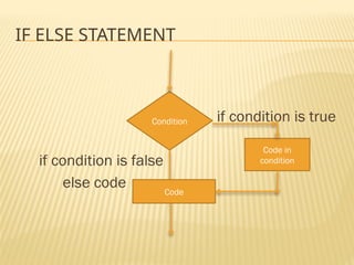
- 19. SET ENVIRONMENT VARIABLE 1. Select “path” variable in system variables 2. Click on edit button 3. Add following path in the path variable C:Users[Your_Current_User_Name]AppData LocalProgramsPythonPython36; Then click on ok Button. Now open command prompt and type python If python shall is running then environment variable is set properly.
- 20. INSATLL IN LINUX Python can be install in Linux in two way 1. By terminal 2. By python.tar.gz file
- 21. BY TERMINAL Open Terminal If you are using Ubuntu 16.10 or newer, then you can easily install Python 3.6 with the following commands # sudo apt-get update # sudo apt-get install python3.6 If you’re using another version of Ubuntu (e.g. the latest LTS release), we recommend using the deadsnakes PPA to install Python 3.6: # sudo apt-get install software-properties-common # sudo add-apt-repository ppa:deadsnakes/ppa # sudo apt-get update # sudo apt-get install python3.6
- 22. INSTALL PYTHON IDLE IN LINUX Run #sudo apt install idle-python3.6 (for python 3.6) Run #idle-python3.6 (for open IDLE)
- 23. PYTHON BASIC SYNTAX Python Identifiers Reserved Words Comments in Python Input output In Python Variable Types Delete variable in python
- 24. PYTHON IDENTIFIERS A Python identifier is a name used to identify a variable, function, class, module or other object. An identifier starts with: A letter A to Z or a to z An underscore (_) followed by zero more letters, Underscores and digits (0 to 9). Python does not allow @, $, and % within identifiers. Python is a case sensitive programming language. White specs not in b/w the catheters E.g. My Name=“mukul”
- 25. RESERVED WORDS and from while assert finally yield break for with class from try continue global return def If Raise elif Import print else In pass is Except or del lambda not
- 26. MULTI-LINE STATEMENTS Statements in Python end with a new line. Even though, allow the use of the line continuation character () to denote that the line should continue. For example − total = item_one + item_two + item_three
- 27. COMMENTS IN PYTHON A hash sign (#) is used to define a comment in python . Python compile ignore the line, which are started from # 1. Single line comment 2. Multiline comment Eg. # Python is a awesome language. “”” Python is a awesome language isn’t it”””
- 28. INPUT OUTPUT IN PYTHON Input: User can give the input to python program by input keyword Ex. i=input() #in python 3.6 Ex. i=raw_input () # in python 2.7 Output: Print keyword is used for print something on monitor Ex. print(“Python is a awesome language”)# in python version 3.6 Print “Python is a awesome language” # in python version 2.7
- 29. VARIABLE TYPES Variables reserved the memory locations to store values. Assignee value to variable counter = 500 # An integer assignment miles = 6000.0 # A floating point name = “Mukul Kirti Verma” # A string Note:- 1.In python no need to define main(). 2.In python no need to define data type for variables.
- 30. MULTIPLE ASSIGNMENT single value to several variables a = b = c = 1 Multiple objects to multiple variables a, b, c = 1,2,"john"
- 31. PYTHON NUMBERS Number data types store numeric values. Number objects are created when you assign a value to them. Ex. var1 = 1 var2 = 10 Python supports three different numerical types − 1. int (signed integers) 2. float (floating point real values) 3. complex (complex numbers)
- 32. DELETE VARIABLE IN PYTHON To delete the reference to a number object by using the del statement. Syntax of the del statement is − del var1,var2,var3,…..,varN Ex. del var1 Delete a single object or multiple objects by using the del statement del var del var_a, var_b
- 33. TYPES OF OPERATOR Python supports the following types of operators: 1.Arithmetic Operators 2.Comparison (Relational) Operators 3.Assignment Operators 4.Logical Operators 5.Bitwise Operators 6.Membership Operators 7.Identity Operators
- 34. ARITHMETIC OPERATORS Operator Example + Addition 2+3=5 -- Subtraction 3-2=1 * Multiplication 2*3=6 / Division 8/2=4 % Modulus (it returns remainder) 3/2=1 ** Exponent (Performs exponential ) 2**3=8 // Floor Division 5//2=2
- 35. COMPARISON OPERATORS Operator Example == compare two values that they are equal or not (a==d) return True if they are equal ,return False if they are not equal != compare two values that they are equal or not (a==d) return False if they are equal ,return True if they are not equal <> Similar to != Similar to != > Compare that left side value is greater then the right side value a>b return true if a is greater then b < Compare that right side value is greater then left side value a<b return true if b is greater then b >= Compare that left side value is greater then or equal to right side value a>=b return true if a is greater then b or equal to b <= Compare that right side value is greater then or equal to left side a<=b return true if a is Lesser then b or equal to b
- 36. ASSIGNMENT OPERATORS = Example = c=a+b it will assigns a+b value to c += c+=a it is equivalent to c=c+a -= c-=a it is equivalent to c=c-a *= c*=a it is equivalent to c=c*a /= c/=a it is equivalent to c=c/a %= c%=a it is equivalent to c=c%a **= c**=a it is equivalent to c=c**a //= c//=a it is equivalent to c=c//a
- 37. BITWISE OPERATORS Operator Example & Binary AND 1 & 0 = 0 | Binary OR 1 | 0 = 0 ^ Binary XOR 1 ^ 0 = 1 ~ Binary Ones complement ~001=1010 >> Binary Right Shift a=2; 2>>1 =1; << Binary Left shift a=2; a<<1=4;
- 38. LOGICAL OPERATORS Operator Example And Logical AND (2<3 and 3>2) return true or Logical OR (2<3 or 3>2) return false Not Logical NOT(2>3) return True
- 39. MEMBERSHIP OPERATORS Operator Example In Return true if it finds a variable in the specified sequence and false if not finds 2 in (2,3,5,6) return true not in Return true if it finds a variable in the specified sequence and false if not finds 2 not in (2,3,5,6) return false
- 40. IDENTITY OPERATORS Operator Example Is Return true if the variables on either side of the operator point to the same object and false otherwise x is y return True if id(x) == d(y) Is not Return false if the variables on the either side of the operator point to the same object and true otherwise X is not y return true if id(x)!=id(y)
- 41. OPERATORS PRECEDENCE S. No. Operator Description (1. Has max prescience and7. has lowest prescience ) 1 peranthsis //(floor division) ** Exponentiation %(Modulo), 2 ~ (complement) 3 (Multiply), /(Division 4 + (Addition) ,-- (subtraction) 5 >>,<< (Right and left bitwise shift) 6 & (Bitwise ‘AND’) 7 ^ (Bitwise XOR), | (regular ‘OR’)
- 42. OPERATORS PRECEDENCE CONTINUE… 8. <= (greater then), <(less then),> (greater then), >= (greater then) 9. <>(not equal to), == (equality operator), != (not equal to) 10. =(equal to), %=, /=, //=, --=, +=, *=, **= (Assignment Operator) 11. is(is operator), is not(is not operator ) 12. in(in Membership operator) not in(not in Membership operator) 13. not (logical not) or(logical or), and(logical and)
- 43. PYTHON TYPE CONVERSION AND TYPE CASTING Type Conversion Implicit Type Conversion Explicit Type Conversion
- 44. TYPE CONVERSION: The process of converting the value of one data type (integer, string, float, etc.) to another data type is called type conversion. Python has two types of type conversion. 1.Implicit Type Conversion 2.Explicit Type Conversion
- 45. IMPLICIT TYPE CONVERSION: In Implicit type conversion, Python automatically converts one data type to another data type. This process doesn't need any user involvement. Let's see an example where Python promotes conversion of lower datatype (integer) to higher data type (float) to avoid data loss. Ex. num_int = 1 num_float = 1.2 num_new = num_int + num_float print("datatype of num_int:",type(num_int))#output:int print("datatype of num_float:",type(num_float))# output:float print("Value of num_new:",num_new) #output:2.2 print("datatype of num_new:",type(num_new))# output:float
- 46. EXPLICIT TYPE CONVERSION: In Explicit Type Conversion, users convert the data type of an object to required data type. We use the predefined functions like int(), float(), str(), etc to perform explicit type conversion. This type conversion is also called typecasting because the user casts (change) the data type of the objects. Syntax : (datatype)(expression) Ex. m=‘3’ print(type(m))#Output: str i=int(m) print(type(i))# Output: int
- 47. INTEGER CONVERSION Int to float Int to complex Int to bool Int to string
- 48. CONTINUE… Syntax: datatype(int) Ex. i=1 j=float(i) #output: 1.0 k=complex(i) #output: 1+0j l=bool(i) #output: True s=str(i) #output:’1’
- 49. CONTINUE… 2.float to other Syntax: datatype(float) 3. bool to other Syntax: datatype(bool) 4. complex to other Syntax: datatype(complex) 5. string to others Syntax: datatype(string)
- 50. KEY POINTS TO REMEMBER: In python type Conversion is the conversion of object from one data type to another data type. Implicit Type Conversion is automatically performed by the Python interpreter. Python avoids the loss of data in Implicit Type Conversion. Explicit Type Conversion is also called Type Casting, the data types of object are converted using predefined function by user. In Type Casting loss of data may occur as we enforce the object to specific data type.
- 51. CONDITION STATEMENTS Three type of conditional statements 1. if 2. if , else (elif) 3. nested if else
- 52. IF STATMENT if condition is true if condition is false Condition Code in condition
- 53. IF STATEMENT EXAMPLE Syntax: if(condition): (code) Example : i=5 If(i<10): print(“Number is Less then 10”) If(i>10): print(“Number is greater then 10”) Output: Number is Less then 10
- 54. IF ELSE STATEMENT if condition is true if condition is false else code Condition Code in condition Code
- 55. CONTINUE…. Syntax: if expression: statement(s) else: statement(s) Example: i=5 If(i<10): print(“Number is lesser then 10”) else: print(“Number is greater then 10”) Output: Number is lesser then 10
- 56. NESTED IF ELSE (ELIF) Syntax: if expression1: statement(s) elif expression2: statement(s) if expression3: statement(s) else: statement(s)
- 57. NESTED IF ELSE (ELIF) Example: var = 1 if var < 2: print (“value is less then 2“) elif (2<=var<=5): print (“number is in b/w 2 and 3“) elif (6<=var<=10): print (“number is in b/w 5 and 10“) elif (11<=var<=15): print (“ number is in b/w 11 and 15“) else: print (“Thank you”) Output: value is less then 2
- 58. PYTHON - LOOPS Loop allow us to execute the set of statement for multiple times. In python three types of loops are define 1. for 2. while 3. nested loop 4. for else 5. while else
- 59. CONTINUE…. It has the ability to iterate over the items of any sequence, such as a list or a string. Syntax: for i in sequence: statements(s)
- 60. CONTINUE…. Example: for letter in ‘mukul': print ('Current Letter :', letter,”n”) Output: Current Letter : m Current Letter : u Current Letter : k Current Letter : u Current Letter : l
- 61. CONTINUE…. Example: fruits = [‘Grapes', 'apple', ‘pineapple'] for fruit in fruits: print( 'Current fruit :', fruit ,’n’ ) Output: Current fruit : Grapes Current fruit : apple Current fruit : pineapple
- 62. WHILE LOOP A while loop statement in Python programming language repeatedly executes a target statement as long as a given condition is true. Syntax: while expression: statement(s)
- 63. Example: count = 0 while (count < 5): print( 'The count is:', count ) count = count + 1 Output: The count is: 0 The count is: 1 The count is: 2 The count is: 3 The count is: 4
- 64. NESTED LOOP 1. Nested for loop 2. Nested while loop
- 65. NESTED FOR LOOP Syntax nested for loop: for iterating_var in sequence: for iterating_var in sequence: statements(s) statements(s)
- 66. NESTED WHILE LOOP Syntax: while expression: while expression: statement(s) statement(s)
- 67. NESTED FOR WHILE LOOP Syntax: for expression: while expression: statement(s) statement(s) or Syntax: while expression: for expression: statement(s) statement(s)
- 68. LOOP CONTROL STATEMENT 1.Break 2.Continue 3.pass
- 69. BREAK STATEMENT It terminates the current loop and resumes execution at the next statement, just like the traditional break. Ex. for letter in ‘Scimox': if letter == ‘m’: break print ('Current Letter :', letter) Output: Current Letter : S Current Letter : c Current Letter : I
- 70. Ex i= 1 while i > 0: print (i) if i== 4: break i=i+1 Output: 1 2 3 4
- 71. CONTINUE STATEMENT It returns the control to the beginning of the while loop.. The continue statement rejects all the remaining statements in the current iteration of the loop and moves the control back to the top of the loop. for letter in ‘Scimox': if letter == ‘m': continue print ('Current Letter :',letter) Output: Current Letter : S Current Letter : c Current Letter : i Current Letter : o Current Letter : x
- 72. Ex. var = 1 while var > 0: var = var +1 if var == 5: continue print (var) if(var==8): break Output: 2 3 4 6 7 8
- 73. PASS STATMENT It is used when you do not want any command or code to execute in loop or control statement or function, etc. The pass statement is a null operation; nothing happens when it executes. Ex. for letter in ‘scimox’: if letter == ‘m’: pass else: print (letter) Output: S C I O X
- 74. STANDARD DATA TYPES Python has five standard data types − Numbers String List Tuple Dictionary
- 75. NUMBERS IN PYTHON Number data types store numeric values. They are immutable data types, means that changing the value of a number data type results in a newly allocated object. var1 = 1 var2 = 10 Python supports Three different numerical types − int (signed integers) float (floating point real values) complex (complex numbers)
- 76. EXAMPLE. Int: 1. i=2 2. i=0x50 Float: 1. i=2.00 2. i=1.22e9 Complex: 1. i=2+5j here 2 is real and 5j is imaginary and j=sqrt (- 1)) 2. i=2j
- 77. MATHEMATICAL FUNCTION Function Description abs() Return absolute value of x exp() exp(x)=(e)power(x) Floor() floor(x) :it Return floor value of x Log() log(x) : it return logarithmic value of x Max() max(x1,x2,x3…,xn) : it return max element in a list Min() min(x1,x2,……xn): it return min element in a list Pow() pow(x,y) : it return x**y Ceil() Return ceiling value
- 78. MATHEMATICAL CONSTRAINTS Sr. No. Constants & Description Example 1 Pi The mathematical constant pi. i=numpy.pi Output : i=3.141592653589793 2 e The mathematical constant e. i=numpy.e Output : i=2.718281828459045
- 79. STRINGS Definition:-String are nothing but set of character. Ex. var1 = ‘Hello scimox' var2 = "Python Programming“ var3=“””hello my name is mukul kirti verma”””
- 80. ACCESSING VALUES IN STRINGS To access substrings, use the square brackets for slicing along with the index or indices to obtain your substring. Ex. string1 = “python is awesome” string2 = “yes it is" print (string2[0] ) Output: ‘py’ print (string2[1:5]) Output: ythoes i
- 81. UPDATE STRINGS Ex var1 = ‘hi my name is xyz‘ print(var1[:6] + ‘mukul’) Output: ‘hi my mukul’ Do not Update a single a char in string like this; var1[14]=‘a’ Print(var1) Output: ‘Error’
- 82. ESCAPE CHARACTERS f to clear screen n for new line r for return t for tab
- 83. STRING METHODS Method capitalize Convert first Character in capital letter center Pads string with specified character casefold converts to casefolded strings count returns occurrences of substring in string endswith Checks if String Ends with the Specified Suffix format formats string into nicer output index Returns Index of Substring isalnum Checks Alphanumeric Character isdecimal Checks Decimal Characters Isdigit Checks Digit Characters isprintable Checks Printable Character
- 84. STRING METHODS Method Description isspace Checks Whitespace Characters istitle Checks for Titlecased String isupper returns if all characters are uppercase characters join Returns a Concatenated String ljust returns left-justified string of given width rjust returns right-justified string of given width swapcase swap uppercase characters to lowercase; vice versa lstrip Removes Leading Characters rstrip Removes Trailing Characters rpartition Returns a Tuple
- 85. STRING METHODS Method Description rindex Returns Highest Index of Substring splitlines Splits String at Line Boundaries rsplit Splits String From Right title Returns a Title Cased String zfile Returns a Copy of The String Padded With Zeros format_map Formats the String Using Dictionary isidentifier Checks for Valid Identifier islower Checks if all Alphabets in a String are Lowercase isnumeric Check whether all element of string in are numeric
- 86. STRING SPECIAL OPERATORS Operator Description + For Concatenation * Repetition [] Slice [ : ] Range Slice in Membership not in Membership r/R Raw String
- 87. ITERATE STRING WITH FOR LOOP str1=“My Name” for j in str1: print(j,”n”) Output: M Y [white space] N a m e
- 88. PYTHON LISTS The list can be written as a collection of comma-separated values (items) between square brackets. Values can be any type of. Eg. list1 = ['physics', 'chemistry', 1997, 2000]; list2 = [1, 2, 3, 4, 5 ]; list3 = ["a", "b", "c", "d"]
- 89. ACCESSING VALUES IN LISTS Ex. list1 = ['physics', 'chemistry', 1997, 2000]; list2 = [1, 2, 3, 4, 5, 6, 7 ]; #printing Single value in list :- Print(list1[0]) Output: ‘physics’ Ex. #print set of continuous values in list print (list2[1:5]) Output: 1,2,3,4
- 90. UPDATING LISTS Ex. list = ['physics', 'chemistry', 1997, 2000]; list[2]=1999 Print(list) Output: ['physics', 'chemistry', 1999, 2000] Ex. list[2:3]=2,3 print (list) Output: ['physics', 'chemistry', 2, 3]
- 91. APPEND ELEMENT IN LIST Ex. List1=[1,2,3] print(List1) Output: [1,2,3] Ex. List1.append(2) Print(list) Output: [1,2,3,2]
- 92. DELETE LIST ELEMENTS Ex. list1 = [‘MUKUL', ‘KIRTI', 1989,2000]; del list1[3]; Print( list1) Output: [‘MUKUL', ‘KIRTI', 1989] But if we execute del list1 Then whole list will be deleted
- 93. OPERATION IN LIST Expression Result list1+list12 It will concatenate list1 and list2 len(list1) It will return length of list1 (‘ok',) * 4 It will return list with 4 element with value ‘ok’ x in (x,y,z) It will check membership of x in list max(list1) It will return max element in list min(list1) It will return min element in list
- 94. TUPLE IN PYTHON A tuple is a sequence of immutable Python objects. Tuples elements cannot be changed Creating a tuple is as simple as putting different comma-separated values in and put in parentheses. Ex. Tuple1=(1,2,3,4,5) Tuple1 = (‘abc', ‘xyz', 1, 3.0); Tuple1 = "a", "b", "c", "d";
- 95. Creating Empty Tuple Tuple1 = (); Creating Tuple with only one value: To create a tuple containing a single value we have to include a comma, even though there is only one value : Tuple1 = (50,);
- 96. ACCESSING VALUES IN TUPLES tup1 = (‘abc', “xyz”, 123, 1.2); tup2 = (1, 2, 3, 4, 5, 6, 7 ); #printing Single value in tuple :- print ("tup1[0]: “,tup1[0]); Output: (‘abc’) # print set of continuous values(tuple slicing) in tuple: print("tup2[1:5]: ", tup2[1:5]); Output: (2,3,4,5)
- 97. UPDATING TUPLES Tuples are immutable which means you cannot update or change the values of tuple elements. tup1 = (12, 34.56); tup1[0] = 100; Output: TypeError: 'tuple' object does not support item assignment
- 98. ADD ELEMEMENT IN TUPLE We can not directly add element in tuple To add element in tuple we need to create a single element tuple the add this tuple to that tuple in which you want to add element. Ex. Tuple1=(1,2,3,4) Tuple2=(5,) Tuple1=Tuple1+Tuple2 Print(Tuple1) Output: (1,2,3,4,5)
- 99. DELETE TUPLE ELEMENTS Because tuple is immutable so element of tuple can not be deleted Only whole tuple can be deleted. Ex. Tuple1=(1,2,3) del Tuple1[0] Output: “Error” Ex. del Tuple1 # now Tuple 1 is deleted Print(Tuple1) Output: NameError: variable name tuple1 not defined
- 100. TUPLES OPERATIONS Expression Result tup1+tup2 It will concatenate tup1 and tup2 len(tup1) It will return length of tup1 (‘ok',) * 4 It will return tuple with 4 element with value ‘ok’ x in (x,y,z) It will check membership of x in tuple max(tup1) It will return max element in tuple min(tup1) It will return min element in tuple count Count element In tuple index Return index of an element in tuple
- 101. DICTIONARY IN PYTHON In python, dictionary is similar to hash or maps in c++. It consists key and value pairs. The value can be accessed by unique key in the dictionary. Keys are unique within a dictionary while values may not be. The values of a dictionary can be of any type, but the keys must be of an immutable data type such as strings, numbers, or tuples. values can be any data type.
- 102. CREATING DECTIONARY Ex. dict1 = {‘2’: ‘4’, ‘3’:’9’ ,’4’:’16’} Print(dict1) Output: {‘2’: ‘4’, ‘3’:’9’ ,’4’:’16’} Ex. dict1 = {‘Man’: ‘Lady’, ‘hen’:’rooster’ ,’cow’:’bull’} print(dict1) Output: {‘Man’: ‘Lady’, ‘hen’:’rooster’ ,’cow’:’bull’} Ex. dict1 = {1: 2, 1.2: 5 ,’cow’:’bull’} print(dict1) Output: {1: 2, 1.2: 5 ,’cow’:’bull’}
- 103. ACCESSING VALUES IN DICTIONARY Ex. dict1 = {‘2': ‘4', ‘3':’9’, ‘4':‘16'} print( dict1[‘2'] ) print ( dict1[‘3'] ) Output: ‘4’ ‘9’ Note: Dictionary Slicing is not possible Means we an not write: dict1[1:3] Output: ‘Error’
- 104. UPDATING DICTIONARY dict1 = {‘1': ‘1', ‘2': 4, ‘3': ‘9'} dict1[‘1'] = “11"; print(dict1) Output: {‘1': ‘11', ‘2': 4, ‘3': ‘9'} dict1[‘2’]=‘44’ Print(dict1) Output: {‘1': ‘11', ‘2': ’44’, ‘3': ‘9'}
- 105. ADDING ELEMENT IN DECTIONARY Ex. dict1 = {‘1': ‘1', ‘2': 4, ‘3': ‘9'} dict1[‘4’]=‘16’ print(dict1) Output: {‘1': ‘1’,‘2': 4,‘3': ‘9‘,’4’:’16’} Ex. dict1[‘5’]=‘25’ print(dict1) Output: {‘1’:’1’,’2’:’4’,’3’:’9’,’4’:’16’,’5’:’25’}
- 106. DELETE DICTIONARY ELEMENTS 1. del dict[‘Key_Name']; # remove entry with key ‘Key_Name‘ 2. dict.clear(); # delete all entries in dict 3. del dict ; # delete entire dictionary
- 107. Ex. dict1 = {‘1': ‘1', ‘2': 4, ‘3': ‘9'} del dict1[‘2’] print(dict1) Output: {‘1': ‘1', ‘3': ‘9'} dict1.clear(); print(dict1) Output: {} del dict1 print(dict1) Output: “NameError: name 'i' is not defined”
- 108. Has key Get Items In len fromkey Update
- 109. BUILT-IN FUNCTIONS & METHODS len(dict) Gives the total length of the dictionary. str(dict) it would convert dictionary in string. type() it would return the type of element of a key passed.
- 110. FUNCTION IN PYTHON A function is a block of code which is run only when, it is called. Creating or defining a Function; def functionname( parameters ): [expression] Ex. def printme(str): print(str) printme(“hi”) Output: ‘hi’
- 111. CALLING A FUNCTION you can execute function code by calling it from another function or directly from the Python prompt. def printme( str ): print str return; printme(“hi")# Output: ‘hi’ printme(“hello") #Output: ‘hello’
- 112. FUNCTION ARGUMENTS A function can be call by using the following types of formal arguments − 1. Required arguments 2. Keyword arguments 3. Default arguments 4. Variable-length arguments
- 113. 1. REQUIRED ARGUMENTS Required arguments are the arguments passed to a function in correct positional order. Here, the number of arguments in the function call should match exactly with the function definition. Ex. # Function definition is here def printme( str ): print str return; #function calling printme() Output: Type Error
- 114. KEYWORD ARGUMENT Keyword arguments are related to the function calls. When you use keyword arguments in a function call, the caller identifies the arguments by the parameter name. def fun( string ): print (string) return; fun( string = "My string")
- 115. CONTINUE… def fun( string1,string2 ): print (string2,string1) return; fun( string2 = “Scimox“,string1=“Cosmo”) Output: “Cosmo” “Scimox”
- 116. DEFAULT ARGUMENTS A default argument is an argument that assumes a default value if a value is not provided in the function call for that argument. def fun( name, Status=“M” ): print (name ,age) return; fun( Status=“S”, name=“Yking" ) fun( name=“Yking”) Output: Yking ,S Yking ,M
- 117. VARIABLE-LENGTH ARGUMENTS You may need to process a function for more arguments than you specified while defining the function. These arguments are called variable- lengtharguments and are not named in the function definition, unlike required and default arguments. Syntax: def function_name(formal_args,*var_args_tuple ): code return [expression]
- 118. LAMBDA FUNCTION(ANONYMOUS FUNCTIONS) These functions are called anonymous because they are not declared in the standard manner by using the def keyword. lambda keyword used to create small anonymous functions. It cantake any number of arguments but return just one value in the form of an expression. They cannot contain commands or multiple expressions. We can cannot direct call to print because lambda requires an expression. It has their own local namespace and it cannot access variables other than their parameter list and those in the global namespace. Although it appears that lambda's are a one-line version of a function, they are not equivalent to inline statements othr languages. whose purpose is by passing function stack allocation during invocation for performance reasons.
- 119. CONTINUE… Syntax: lambda [arg1 ,arg2,.....argn]: expression Ex. sum = lambda arg1, arg2,arg3: arg1 + arg2+arg3; X=sum(5, 5, 5 ) Y=sum( 5000, 5000, 5000 ) print(X,”,”,Y) Output: 15 , 15000
- 120. RETURN STATEMENT The statement return statement quit a function, and optionally passing back an expression to its caller. A return statement with no arguments returns none. Ex. def sum( arg1, arg2 ): total = arg1 + arg2 print (sum( 5, 5 )); print (sum) Output: 10 10
- 121. SCOPE OF VARIABLES There are two basic scopes of variables in python 1. Global variables 2. Local variables Ex. total = 0 This is global variable. def sum( arg1, arg2 ): total = arg1 + arg2 print( total ) return total sum( 10, 20 ) print ( total ) Output: 30 0
- 122. RECURSIVE FUNCTION Recursion is the calling of function to itself. A physical world example would be to place two parallel mirrors facing each other. Any object in between them would be reflected recursively. Ex. def sum(list): sum = 0 def sum(list): # Add every number in the list if len(list) == 1: for i in range(0, len(list)): return list[0] sum = sum + list[i] else: return list[0]+sum(list[1:]) return sum print(sum([5,7,3,8,10])) print(sum([5,7,3,8,10])) Output:33 Output:33
- 123. CONTINUE… Advantages of Recursion Recursive functions make the code look clean and elegant. A complex task can be broken down into simpler sub-problems using recursion. Sequence generation is easier with recursion than using some nested iteration. Disadvantages of Recursion Sometimes the logic behind recursion is hard to follow through. Recursive calls are expensive (inefficient) as they take up a lot of memory and time. Recursive functions are hard to debug.
- 124. BINARY NUMBERS This tiny amount of information, the smallest amount of information that you can store in a computer, is known as a bit. We represent a bit as either low (0) or high (1). Topics: 1. Convert binary to other base 2. Logical operations
- 125. CONVERT BINARY TO OTHER BASE Binary to other base Syntax: int(binary number, base) Ex. Binary to decimal(base 2) int(“1001”,2) Output: 9 Binary to base 3 int(“1001”,3) Output: 28 Binary to base 4 int(“1001”,4) Output: 65 Binary to base 5 int(“1001”,5) Output: 126
- 126. LOGICAL OPERATIONS 1. AND 2. OR 3. XOR 4. bitwise left shift 5. bitwise right shift
- 127. 1. AND (&) Ex. X=1 Y=1 Print(x&y) Output: 1 Ex. inputA = int('00100011',2) inputB = int('00101101',2) print (bin(inputA & inputB)) Output: 0b1100
- 128. BITWISE OR(|) 1. OR (|) Ex. X=1 Y=1 Print(x|y) Output: 1 Ex. inputA = int('00100011',2) inputB = int('00101101',2) print (bin(inputA & inputB)) Output: 0b111101
- 129. BITWISE XOR(|) 1. XOR (^) Ex. X=1 Y=1 Print(x^y) Output: 0 Ex. inputA = int('00100011',2) inputB = int('00101101',2) print (bin(inputA ^ inputB)) Output: 0b110001
- 130. LEFT SHIFT Left Sift(>>) Syntax: Binary_number>>Number of bit to be shift Ex. Print(5>>2) Output: 1 Ex. Print(5>>1) Output: 2
- 131. RIGHT SHIFT Right Sift(>>) Syntax: Binary_number<<Number of bit to be shift Ex. Print(5<<2) Output: 20 Ex. Print(5<<1) Output: 10
- 132. MODULES Consider a module to be the same as a code library. A file containing a set of functions you want to include in your application. a module is a file consisting of Python code. A module can define functions, classes and variables. A module can also include runnable code. Steps: 1. Make Module 2. Import Module I your code
- 133. CREATE MODULE 1. create a file 2. write your code in that file def print_sum( x,y ): print (x+y) return def print_sub( x-y ): print (x-y) return 3. save this file as .py file Ex. save as this file modul1.py
- 134. IMPORT MODULE Syntax: import module1, module2,... moduleN Ex. import module1 X=module1.print_sum(4,5) Y=module1.print_sub(4,5) Output: 9 -1
- 135. FROM...IMPORT STATEMENT From statement lets you enable to import specific attributes from a module into the current prog. Syntax: from module_name import name1, name2, ... nameN Ex. from module1 import sum print(sum(2,3)) #output: 5 print(module1.sub(2,5)) # output: Error
- 136. THE FROM...IMPORT * STATEMENT It is also possible to import all names from a module into the current namespace using instead of attribute name*: Syntax: from module_name import * Ex. from module1 import * X=sum(2,3) output: 5 Y=sub(2,3) output: -1
- 137. PACKAGES IN PYTHON A package is a hierarchical file directory structure that defines a single Python application environment that consists of modules and subpackages and sub- subpackages, and so on. Ex. Numpy,pandas, sklearn,matplotlib ramdom.
- 138. INSTALL THE PACKAGE IN PYTHON To install package in python you need to run the following command in operating system command prompt. Step 1. open command prompt 2. run : #pip install numpy It will install numpy in your system. now you can use this numpy package in your program. Similarly you can install other packages.
- 139. To install package In spyder and other IDE in your anaconda environment you have two options. 1. By python prompt 2. By anaconda GUI.
- 140. DATE TIME To use datetime in python first we need to install and import the datetime library in your program import datetime To import library first we need to download and install library in your system. To install library type following command in command prompt: $pip install datetime After that datetime library will install in your system. And now import library in your program by typing line: $Import datetime Now you can use datetime function in your program
- 141. DATETIME CLASSES Datetime.date Attributes: year, month, and day. Datetime.time Attributes: hour, minute, second, microsecond, and tzinfo. Datetime.datetime Attributes: year, month, day, hour, minute, second, microsecond, and tzinfo. Datetime.timedelta A duration expressing the difference between two date, time, or datetime instances to microsecond resolution. Datetime.tzinfo These are used by the datetime and time classes to provide a customizable notion of time adjustment (for example, to account for time zone and/or daylight saving time). Datetime.timezone A class that implements the tzinfo abstract base class as a fixed offset from the UTC.
- 142. DATETIME.DATE METHODS 1. Create a date import datetime Syntax: datetime.date(year,mon,day) All arguments are optional and default to 0. Arguments may be ints, or floats, and may be positive or negative. d=datetime.date(2002,7,23) print(d) Output: 2002-07-23 2. Print Today's Date today=datetime.date.today() Print(today) Output: 2018/7/27
- 143. DATETIME.DATE METHODS import datetime today=datetime.date.today()# it will create todays date print(today)#Output: 2018-07-27 print(today.day)#Output: 27 print(today.month) )#Output: 07 print(today.year)#Output: 2018 print(today.weekday())#Output: 4 print(today.isoweekday())#Output: 5 Note: 1.for weekday():- Mo:0, Tu:1, We:2, Thu:3, Fri:4, sat:5, sun:6 2.for isoweekday() Mo:1, Tu:0, We:3, Thu:4, Fri:5, sat:6, sun:7
- 144. DATETIME.TIME METHODS Creating time Syntax: datetime.time(hour, minute, second, microsecond, and tzinfo.) All arguments are optional and default to 0. Arguments may be ints, or floats, and may be positive or negative. t=datetime.time(9,30,45,100000) print(t.hour) # Output: 9 print(t.minute) # Output: 30 print(t.second) # Output: 45 print(t.microsecond) # Output: 10000
- 145. DATETIME.DATETIME METHODS Creating datetime Syntax: datetime.datetime(year,mon,day,hour, minute, second, microsecond, tzinfo) All arguments are optional and default to 0. Arguments may be ints, or floats, and may be positive or negative. t=datetime.datetime(2002,07,23,9,30,45,100000) print(t.hour) # Output: 9 print(t.minute) # Output: 30 print(t.second) # Output: 45 print(t.microsecond) # Output: 10000 print(today.day)#Output: 23 print(today.month) )#Output: 07 print(today.year)#Output: 2002 print(today.weekday())#Output: 1 print(today.isoweekday())#Output: 2
- 146. DATETIME.TIMEDELTA METHODS A timedelta object represents a duration, the difference between two dates or times. datetime.timedelta(days, seconds, microseconds, milliseconds, minutes, hour s, weeks) All arguments are optional and default to 0. Arguments may be ints, or floats, and may be positive or negative. Only days, seconds and microseconds are stored internally. Arguments are converted to those units: A millisecond is converted to 1000 microseconds. A minute is converted to 60 seconds. An hour is converted to 3600 seconds. A week is converted to 7 days.
- 147. TIMEDELTA 1. Substract and add few days from date Sub and Add 7 days in todays date where today date is 7/27/2018) tdelta=datetime.timedelta(days=7) print(tdelta) #Output: 7 days, 0:00:00 date2=datetime.today()+tdelta print(date2)#Output:08/03/2018 date2=datetime.today()-tdelta print(date2)#Output: 07/20/2018 2. Add time in date t=datetime.datetime(2016,7,30,12,30,45,10000) tdelta=datetime.timedelta(hours=20) print(t+tdelta) Output:2016-07-31 08:30:45.010000 Print(t-tdelta) Output:2016-07-29 16:30:45.010000
- 148. UTC(UNIVERSAL TIME COORDINATE) TIMEZONE 1. Find universal time zone dt_utcnow=datetime.datetime.utcnow() 2. find time in india from UTC time. dt_utcnow=datetime.datetime.utcnow() print(dt_utcnow)#output: 7/27/2018 11:28 AM t=datetime.timedelta(hours=5.5) t_india=dt_utcnow+t Print(t_india) 7/27/2018 4:58 PM
- 149. SETS A set is a collection which is ordered and unindexed. In Python sets are written with curly brackets. 1. Crating sets 2. Using the set() constructor to make a set 3. Add element in set 4. Remove element in set 5. length of set
- 150. 1. Creating set x= {“A", “B", “C"} print(x) 2. Using set() constructor: x = set(("apple", "banana", "cherry")) print(x)
- 151. 3. add() method to add an item in set: x= set(("apple", "banana", "cherry")) x.add("damson") print(x) 4. remove() method to remove an item in set: x = set(("apple", "banana", "cherry")) x.remove("banana") print(x) 5. length() method to find length of set x = set(("apple", "banana", "cherry")) print(len(x)) Output: 3
- 152. RANDOM NUMBER random()-Return the next random floating point number in the range (0.0, 1.0) random.randint(start,end)-Returns a random integer between a and b inclusive random.sample(list,int)-Return a k length list of unique elements chosen from the population sequence. random.uniform(start,end)-Return a random floating point number between a and b inclusive. random.getrandbits(k)-Returns a Python integer with k random bits. random.randrange(start, stop)-Returns a random integer from the range. random.choice(seq)-Return a random element from the non-empty sequence.
- 153. PANDAS Create dataset Get Data Prepare Data Analyze Data
- 154. OBJECT CREATION 1. Series creation 2. DataFrame creation 1. Series creation Syntax: panda.series(data) Ex. Import pandas as pd i=pd.series([1,3,5,7,6,8]) print(i) Print(type(i)) Output: 0 1 1 3 2 5 3 7 4 6 5 8 dtype: int64 series
- 155. CREATING DATAFRAME Syntax: pd.DataFrame(data, index,columns) Ex. Import panda as pd Import numpy as np Index1=[1,2,3,4,5,6] df = pd.DataFrame(np.random.randn(6,1), index=index1, columns=list('A')) print(df) Output: A 1 0.112 2 0.222 3 0.255 4 0.523 5 0.232 6 0.112
- 156. Ex. df2 = pd.DataFrame ({ 'A' : 1, 'B' : pd.Timestamp('20130102'), 'C' : pd.Series(1,index=list(range(4)),dtype='float32'), 'D' : np.array([3] * 4,dtype='int32'), 'E' : pd.Categorical(["test","train","test","train"]}), print(df2) Output: A B C D E 0 1.0 2013-01-02 1.0 3 test 1 1.0 2013-01-02 1.0 3 train 2 1.0 2013-01-02 1.0 3 test 3 1.0 2013-01-02 1.0 3 train 4 1.0 2013-01-02 1.0 3 test 5 1.0 2013-01-02 1.0 3 train
- 157. df2.dtypes Output A float64 B datetime64[ns] C float32 D int32 E category
- 158. VIEWING DATA df.head() Here is how to view the top 5 rows of the frame: df.head() Output: A B C D E 0 1.0 2013-01-02 1.0 3 test 1 1.0 2013-01-02 1.0 3 train 2 1.0 2013-01-02 1.0 3 test 3 1.0 2013-01-02 1.0 3 train 4 1.0 2013-01-02 1.0 3 test
- 159. df.head(3) Output: A B C D E 0 1.0 2013-01-02 1.0 3 test 1 1.0 2013-01-02 1.0 3 train 2 1.0 2013-01-02 1.0 3 test
- 160. df.tail() Here is how to view the bttom 5 rows of the frame: df.tail() Output: A B C D E 1 1.0 2013-01-02 1.0 3 train 2 1.0 2013-01-02 1.0 3 test 3 1.0 2013-01-02 1.0 3 train 4 1.0 2013-01-02 1.0 3 test 5 1.0 2013-01-02 1.0 3 train
- 161. DISPLAY THE INDEX, COLUMNS df.index Output: 0 1 2 3 4 5
- 162. df.columns Output: Index(['A', 'B', 'C', 'D‘,’E’], dtype='object') df.values Output: array[1.0 2013-01-02 1.0 3 train 1.0 2013-01-02 1.0 3 test 1.0 2013-01-02 1.0 3 train 1.0 2013-01-02 1.0 3 test 1.0 2013-01-02 1.0 3 train]
- 163. df.head(2).T Output: 0 1 A 1.0 1.0 B 2013-01-02 2013-01-02 C 1.0 1.0 D 3 3 E test train
- 164. df.sort_index(axis=1, ascending=False) df.sort_values(by='B')
- 165. SELECTION 1.select single column print(df[‘A’]) Output: A 1 1.0 2 1.0 3 1.0 4 1.0 5 1.0 Freq: D, Name: A, dtype: float64
- 166. Select multiple column Syntax: df1=df.loc[:,['A','B']] Print(df1) Output: A B 0 1.0 2013-01-02 1 1.0 2013-01-02 2 1.0 2013-01-02 3 1.0 2013-01-02 4 1.0 2013-01-02
- 167. Select rows df[start_row_index : end_row_index, colum] Ex. df[1 : 3] Output: A B C D E 1 1.0 2013-01-02 1.0 3 test 2 1.0 2013-01-02 1.0 3 train 3 1.0 2013-01-02 1.0 3 test
- 168. Select multiple rows with index value df[1:3] Output: A B C D E 1 1.0 2013-01-02 1.0 3 test 2 1.0 2013-01-02 1.0 3 train
- 169. Selection by Label df.loc[index] Output: 0 A 1.0 B 2013-01-02 C 1.0 D 3 E test
- 170. Selecting on a multi-axis by label df.loc[1:3,['A','B']] Output: A B 1 1.0 2013-01-02 2 1.0 2013-01-02
- 171. Select row df.iloc[0] Output: 0 A 1.0 B 2013-01-02 C 1.0 D 3 E test
- 172. Select multiple rows df.iloc[0:2] A B C D E 0 1.0 2013-01-02 1.0 3 train 1 1.0 2013-01-02 1.0 3 test]
- 173. getting fast access to a scalar (equivalent to the prior method): df.iat[1,1] Output: 2013-01-02
- 174. UPDATE IN DARAFRAME Updat vealues by label: df.at[index,'A'] = 0.0 print(df) Output: A B C D E 0 0.0 2013-01-02 1.0 3 test 1 1.0 2013-01-02 1.0 3 train 2 1.0 2013-01-02 1.0 3 test 3 1.0 2013-01-02 1.0 3 train 4 1.0 2013-01-02 1.0 3 test
- 175. Setting a new column automatically aligns the data by the indexes s1 = pd.Series([11,12,13,14,15,16] ,index=[0,1,2,3,4,5]) df[‘F’]=s1 Print(df) Output: A B C D E F 0 1.0 2013-01-02 1.0 3 test 11 1 1.0 2013-01-02 1.0 3 train 12 2 1.0 2013-01-02 1.0 3 test 13 3 1.0 2013-01-02 1.0 3 train 14 4 1.0 2013-01-02 1.0 3 test 15
- 176. Update values by position: df.iat[0,1] = 0 print(df) Output; A B C D E 0 1.0 0 1.0 3 test 1 1.0 2013-01-02 1.0 3 train 2 1.0 2013-01-02 1.0 3 test 3 1.0 2013-01-02 1.0 3 train 4 1.0 2013-01-02 1.0 3 test
- 177. Add row in dataframe: s1 = pd.Series([11,12,13,14,15,16]) dft=pd.DataFrame(data=sum_row).T dft=dft.reindex(columns=df.columns) df_final=df.append(dft,ignore_index=True) print(df) Output: A B C D E 0 1.0 2013-01-02 1.0 3 test 1 1.0 2013-01-02 1.0 3 train 2 1.0 2013-01-02 1.0 3 test 3 1.0 2013-01-02 1.0 3 train 4 1.0 2013-01-02 1.0 3 test 5 11 12 13 14 15
- 178. Insert a column Syntax df.insert(column no, column header, data) df.insert(4, “col7", np.nan) print(df) Output: A B C D E col7 0 1.0 2013-01-02 1.0 3 test np.nan 1 1.0 2013-01-02 1.0 3 train np.nan 2 1.0 2013-01-02 1.0 3 test np.nan 3 1.0 2013-01-02 1.0 3 train np.nan 4 1.0 2013-01-02 1.0 3 test np.nan
- 179. READING CSV AND TEXT FILE Reading CSV file Syntax: df=pd.read_table(r“file_pathfile_name(including “.csv”)) Ex. df=pd.read_table(r“c:usersskydesktoprefinedCCD2.csv”)) Or df=pd.read_csv(r“c:usersskydesktoprefinedCCD2.csv”)) Print(df) Output: DT1 RHOB1 MD 0 66 2006 300 1 200 2384 200640
- 180. READING CSV FILE Syntax: df=pd.read_table(r“file_pathfile_name(including “.txt”)) Ex. df=pd.read_table(r“c:usersskydesktoprefinedCCD2.txt”)) Or df=pd.read_csv(r“c:usersskydesktoprefinedCCD2.txt”)) Print(df) Output: Exception Handling 0 Intro to Exception 1 Handl an exception 2 Handle Multiple Exceptions 3 The try-finally Clause 4 Exception Arguments 5 Raising an Exceptions
- 181. WRITING DATAFRAME TO CSV OR TEXT FILE Import panda as pd Import numpy as np Index1=[1,2,3,4,5,6] df = pd.DataFrame(np.random.randn(6,1), index=index1, columns=list('A')) df.to_csv('new.csv', sep='t')#to create csv file df.to_csv('new.txt', sep='t')#to create text file Output; new.csv new.txt
- 182. MATPLOTLIB GRAPH PLOTING 1. sipmle chart 2. bar chart 3. histogram 4. box 5. area 6. scatterd 7. pie chart
- 183. SIMPLE CHART import pandas as pd import numpy as np import matplotlib.pyplot as plt ts1=pd.Series([x*x for x in range(1,30)]) ts1.plot() Output:
- 184. MULTIPLE SIPMLE GRAPH IN SINGLE FRAME Import panda as pd Import numpy as np import matplotlib.pyplot as plt ts1=pd.Series([x*x for x in range(1,30)]) ts2=pd.Series([x*x*x for x in range(1,30)]) df=pd.DataFrame() df.insert(0, "ts1", ts1) df.insert(1, "ts2", ts2) plt.figure(); plt.set_xlabel(“x”);plt.set_ylabel(“y”) df.plot();
- 185. OUTPUT:
- 186. BAR CHART df = pd.DataFrame(data=np.random.randn(1000, 4), columns=list('ABCD')) df.iloc[5].plot(kind='bar');
- 187. MULTIPLE BAR CHART df.head().plot(kind='bar');
- 188. STACKED BAR CHART df2 = pd.DataFrame(np.random.rand(10, 4), columns=['a', 'b', 'c', 'd']) df2.plot.bar(stacked=True);
- 189. STACKED HORIZONTAL BAR CHART df2 = pd.DataFrame(np.random.rand(10, 4), columns=['a', 'b', 'c', 'd']) df2.plot.barh(stacked=True);
- 190. HISHTOGRAM df4 = pd.DataFrame(np.random.randn(1000) ,colum ns=['a']) plt.figure(); df4['a'].hist()
- 191. Set color df4['c'].hist(color='red')
- 192. MULTPLE HISTOGRAM df4 = pd.DataFrame({'a': np.random.randn(1000) , 'b': np.random.randn(1000),'c': np.random.randn(1000)}, columns=['a', 'b', 'c']) df4.plot.hist()
- 193. Set opecity df4.plot.hist( alpha=0.3)
- 195. BOX PLOT df = pd.DataFrame(np.random.rand(10), columns=['A']) df['A'].plot.box()
- 196. SET COLOR df = pd.DataFrame(np.random.rand(10, 5), columns=['A', 'B', 'C', 'D', 'E']) color = dict(boxes='DarkGreen', whiskers='DarkOrange',medians='DarkBlue', caps='Gray')
- 197. VERTICAL BOX PLOT df.plot.box(vert=False)
- 198. SCATERD CHART df = pd.DataFrame(np.random.rand(50, 4), columns=['a', 'b', 'c','d']) df.plot.scatter(x='a', y='b');
- 199. PIE CHART series = pd.Series(3 * np.random.rand(4), index=['a', 'b', 'c', 'd'], name='series') series.plot.pie()
- 200. COMPARE DATA WITH PIE CHART df = pd.DataFrame(np.random.rand(4, 2), index=['a', 'b', 'c', 'd'], columns=['x', 'y']) df.plot.pie(subplots=True, figsize=(8, 4))
- 201. NUMPY ARRAY Array is a collection of similar data types’. 1. Install numpy Run: pip install numpy 2. Import numpy in your code import numpy as np
- 202. CREATE NUMPY ARRAY 1. Create 1D Array 2. Create 2D Array 1. Create 1D Array Ex. import numpy as np a = np.array([1, 2, 3, 4]) Print( a ) Output: [1,2,3,4]
- 203. 2. CREATE 2D ARRAY Ex.1 import numpy as np a = np.array([[1, 2], [3, 4]]) print (a) Output: [[1,2], [3,4]] Ex.2 import numpy as np a = np.array([[1, 2, 5 ], [3, 4, 6]]) print (a) Output: [[1,2, 5], [3,4, 6]]
- 204. SOME METHODS: 1. dtype() 2. shape() 3. Range() 4. itemsize() 5. zeros() 6. ones() 7. asarray() 8. linspace() 9. logspace 10. endpoint()
- 205. 1. DATATYPE PARAMETER 1. Datatype parameter (dtype()) import numpy as np a = np.array([1, 2, 5], dtype = complex) Print( a ) Output: [ 1.+0.j, 2.+0.j, 5.+0.j] 2. Reshape Array(array.shape) import numpy as np a = np.array([[1,2,3],[4,5,6]]) print (a.shape) Output: (2,3) a.shape = (3,2) Print( a ) Output: [[1, 2] [3, 4] [5, 6]]
- 206. RANGE() Ex. import numpy as np a = np.arange(10) print( a ) Output; [1,2,3,4,5,6,7,8,9,10] Ex. import numpy as np a = np.arange(24) a.ndim b = a.reshape(2,4,3) print (b) Output: [[[ 0, 1, 2] [ 3, 4, 5] [ 6, 7, 8] [ 9, 10, 11]] [[12, 13, 14] [15, 16, 17] [18, 19, 20] [21, 22, 23]]]
- 207. ITEMSIZE() This array attribute returns the length of each element of array in bytes. Ex. import numpy as np x = np.array([1,2,3,4,5], dtype = np.int8) print (x.itemsize) Output: 1 Ex. import numpy as np x = np.array([1,2,3,4,5], dtype = np.float32) print (x.itemsize) Output: 4
- 208. ZERO() To create array of n zeros & Default dtype is float. Ex. import numpy as np x = np.zeros(6) print (x) Output: [0.,0.,0.,0.,0.,0.] x.shap=(2,3) Output: [[0.,0.,0.], [0.,0.,0,]]
- 209. ONES() Ex. import numpy as np x = np.ones(5) print (x) Output: [1.,1.,1.,1.,1.,] x.shap=(2,3) Output: [[1.,1.,1.], [1.,1.,1,]]
- 210. ASARRAY() This function is similar to numpy.array except for the fact that it has fewer parameters. This routine is useful for converting Python sequence into ndarray. Ex. import numpy as np x = [1,2,3] a = np.asarray(x) print( a ) Output: [1 2 3]
- 211. Ex. 2 import numpy as np x = [1,2,3] a = np.asarray(x, dtype = float) Print( a ) Output: [1,2,3] Ex.3 # ndarray from tuple import numpy as np x = (1,2,3) a = np.asarray(x) print (a) Output: [1,2,3]
- 212. LINSPACE() Syntax: numpy.linspace(start, stop, num, endpoint, retstep, dtype) Ex. import numpy as np x = np.linspace(10,20,5) print(x) Output: [10. 12.5 15. 17.5 20.]
- 213. Endpoint set to false : import numpy as np x = np.linspace(10,20, 5, endpoint = False) print( x ) Output: [10. 12. 14. 16. 18.] Find retstep value : import numpy as np x = np.linspace(1,3,4, retstep = True) print (x) # retstep here is 0.25 Output; (array([ 1. , 1.25, 1.5 , 1.75, 2. ]), 0.25)
- 214. LOGSPACE() Syntax: numpy.logspace(start, stop, num, endpoint, base, dtype) Ex. import numpy as np a = np.logspace(1.0, 2.0, num = 10) print (a) Output: [ 10. 12.91549665 16.68100537 21.5443469 27.82559402 35.93813664 46.41588834 59.94842503 77.42636827 100. ]
- 215. Ex. set base of log space to 2 import numpy as np a = np.logspace(1,10,num = 10, base = 2) print (a) Output: [ 2. 4. 8. 16. 32. 64. 128. 256. 512. 1024.]
- 216. INDEXING & SLICING (VALUE ACCESS) 1. slice single item 2. slice Multiple item 3. slice items starting from index 4. slice items between indexes 5. slice items starting from index 6. slice column 7. slice Row
- 217. 1. SLICE SINGLE ITEM # slice single item import numpy as np a = np.arange(10) b = a[4] print (b) Output: 4
- 218. 1. SLICE SINGLE ITEM import numpy as np a = np.arange(10) s = slice(2,7,2)# (start , end ,step) and work in python2.7 print (a[s]) Output: [2 4 6]
- 219. Ex. import numpy as np a = np.arange(10) b = a[2:7:2] #in python 3.5 & above print (b) Output: [2,4,6]
- 220. SLICE ITEMS STARTING FROM INDEX Ex. import numpy as np a = np.arange(10) print (a[2:]) Output: [2 3 4 5 6 7 8 9]
- 221. SLICE ITEMS BETWEEN INDEXES Ex. import numpy as np a = np.arange(6) print (a[2:5]) Output: [2 3 4]
- 222. SLICE ITEMS STARTING FROM INDEX import numpy as np a = np.array([[1,2,3],[3,4,5],[4,5,6]]) print(a) Output: [[1, 2, 3], [3, 4, 5], [4, 5, 6]] print a[1:] Output: [[3 4 5] [4 5 6]]
- 223. COLUMN SLICING Ex. import numpy as np a = np.array([[1,2,3],[3,4,5],[4,5,6]]) print (a) Output: [[1,2,3], [3,4,5], [4,5,6]] print (a[...,1] ) Output: [2 4 5]
- 224. ROW SLICING Ex. import numpy as np a = np.array([[1,2,3],[3,4,5],[4,5,6]]) print (a) Output: [[1,2,3], [3,4,5], [4,5,6]] print (a[1,...] ) Output: [3 4 5]
- 225. Method/ AttributePurpose match() Determine if the RE matches at the beginning of the string.search()Scan through a string, looking for any location where this RE matches.findall()Find all substrings where the RE matches, and returns them as a list.finditer()Find all substrings where the RE matches, and returns them as an iterator.
Editor's Notes
- #155: x