Quicksort and MergeSort Algorithm Analysis

1. Mergesort and Quicksort Chapter 8 Kruse and Ryba

2. Sorting algorithms • Insertion, selection and bubble sort have quadratic worst-case performance • The faster comparison based algorithm ? O(nlogn) • Mergesort and Quicksort

3. Merge Sort • Apply divide-and-conquer to sorting problem • Problem: Given n elements, sort elements into non-decreasing order • Divide-and-Conquer: – If n=1 terminate (every one-element list is already sorted) – If n>1, partition elements into two or more sub- collections; sort each; combine into a single sorted list • How do we partition?

4. Partitioning - Choice 1 • First n-1 elements into set A, last element set B • Sort A using this partitioning scheme recursively – B already sorted • Combine A and B using method Insert() (= insertion into sorted array) • Leads to recursive version of InsertionSort() – Number of comparisons: O(n2 ) • Best case = n-1 • Worst case = 2 ) 1 ( 2     n n i c n i

5. Partitioning - Choice 2 • Put element with largest key in B, remaining elements in A • Sort A recursively • To combine sorted A and B, append B to sorted A – Use Max() to find largest element  recursive SelectionSort() – Use bubbling process to find and move largest element to right-most position  recursive BubbleSort() • All O(n2 )

6. Partitioning - Choice 3 • Let’s try to achieve balanced partitioning • A gets n/2 elements, B gets rest half • Sort A and B recursively • Combine sorted A and B using a process called merge, which combines two sorted lists into one – How? We will see soon

7. Example • Partition into lists of size n/2 [10, 4, 6, 3] [10, 4, 6, 3, 8, 2, 5, 7] [8, 2, 5, 7] [10, 4] [6, 3] [8, 2] [5, 7] [4] [10] [3][6] [2][8] [5][7]

8. Example Cont’d • Merge [3, 4, 6, 10] [2, 3, 4, 5, 6, 7, 8, 10 ] [2, 5, 7, 8] [4, 10] [3, 6] [2, 8] [5, 7] [4] [10] [3][6] [2][8] [5][7]

9. Static Method mergeSort() Public static void mergeSort(Comparable []a, int left, int right) { // sort a[left:right] if (left < right) {// at least two elements int mid = (left+right)/2; //midpoint mergeSort(a, left, mid); mergeSort(a, mid + 1, right); merge(a, b, left, mid, right); //merge from a to b copy(b, a, left, right); //copy result back to a } }

10. Merge Function

11. Evaluation • Recurrence equation: • Assume n is a power of 2 c1 if n=1 T(n) = 2T(n/2) + c2n if n>1, n=2k

12. Solution By Substitution: T(n) = 2T(n/2) + c2n T(n/2) = 2T(n/4) + c2n/2 T(n) = 4T(n/4) + 2 c2n T(n) = 8T(n/8) + 3 c2n T(n) = 2i T(n/2i ) + ic2n Assuming n = 2k , expansion halts when we get T(1) on right side; this happens when i=k T(n) = 2k T(1) + kc2n Since 2k =n, we know k=logn; since T(1) = c1, we get T(n) = c1n + c2nlogn; thus an upper bound for TmergeSort(n) is O(nlogn)

13. Quicksort Algorithm Given an array of n elements (e.g., integers): • If array only contains one element, return • Else – pick one element to use as pivot. – Partition elements into two sub-arrays: • Elements less than or equal to pivot • Elements greater than pivot – Quicksort two sub-arrays – Return results

14. Example We are given array of n integers to sort: 40 20 10 80 60 50 7 30 100

15. Pick Pivot Element There are a number of ways to pick the pivot element. In this example, we will use the first element in the array: 40 20 10 80 60 50 7 30 100

16. Partitioning Array Given a pivot, partition the elements of the array such that the resulting array consists of: 1. One sub-array that contains elements >= pivot 2. Another sub-array that contains elements < pivot The sub-arrays are stored in the original data array. Partitioning loops through, swapping elements below/above pivot.

17. 40 20 10 80 60 50 7 30 100 pivot_index = 0 [0] [1] [2] [3] [4] [5] [6] [7] [8] too_big_index too_small_index

18. 40 20 10 80 60 50 7 30 100 pivot_index = 0 [0] [1] [2] [3] [4] [5] [6] [7] [8] too_big_index too_small_index 1. While data[too_big_index] <= data[pivot] ++too_big_index

21. 40 20 10 80 60 50 7 30 100 pivot_index = 0 [0] [1] [2] [3] [4] [5] [6] [7] [8] too_big_index too_small_index 1. While data[too_big_index] <= data[pivot] ++too_big_index 2. While data[too_small_index] > data[pivot] --too_small_index

22. 40 20 10 80 60 50 7 30 100 pivot_index = 0 [0] [1] [2] [3] [4] [5] [6] [7] [8] too_big_index too_small_index 1. While data[too_big_index] <= data[pivot] ++too_big_index 2. While data[too_small_index] > data[pivot] --too_small_index

23. 40 20 10 80 60 50 7 30 100 pivot_index = 0 [0] [1] [2] [3] [4] [5] [6] [7] [8] too_big_index too_small_index 1. While data[too_big_index] <= data[pivot] ++too_big_index 2. While data[too_small_index] > data[pivot] --too_small_index 3. If too_big_index < too_small_index swap data[too_big_index] and data[too_small_index]

24. 40 20 10 30 60 50 7 80 100 pivot_index = 0 [0] [1] [2] [3] [4] [5] [6] [7] [8] too_big_index too_small_index 1. While data[too_big_index] <= data[pivot] ++too_big_index 2. While data[too_small_index] > data[pivot] --too_small_index 3. If too_big_index < too_small_index swap data[too_big_index] and data[too_small_index]

25. 40 20 10 30 60 50 7 80 100 pivot_index = 0 [0] [1] [2] [3] [4] [5] [6] [7] [8] too_big_index too_small_index 1. While data[too_big_index] <= data[pivot] ++too_big_index 2. While data[too_small_index] > data[pivot] --too_small_index 3. If too_big_index < too_small_index swap data[too_big_index] and data[too_small_index] 4. While too_small_index > too_big_index, go to 1.

31. 1. While data[too_big_index] <= data[pivot] ++too_big_index 2. While data[too_small_index] > data[pivot] --too_small_index 3. If too_big_index < too_small_index swap data[too_big_index] and data[too_small_index] 4. While too_small_index > too_big_index, go to 1. 40 20 10 30 7 50 60 80 100 pivot_index = 0 [0] [1] [2] [3] [4] [5] [6] [7] [8] too_big_index too_small_index

40. 1. While data[too_big_index] <= data[pivot] ++too_big_index 2. While data[too_small_index] > data[pivot] --too_small_index 3. If too_big_index < too_small_index swap data[too_big_index] and data[too_small_index] 4. While too_small_index > too_big_index, go to 1. 5. Swap data[too_small_index] and data[pivot_index] 40 20 10 30 7 50 60 80 100 pivot_index = 0 [0] [1] [2] [3] [4] [5] [6] [7] [8] too_big_index too_small_index

42. Partition Result 7 20 10 30 40 50 60 80 100 [0] [1] [2] [3] [4] [5] [6] [7] [8] <= data[pivot] > data[pivot]

43. Recursion: Quicksort Sub-arrays 7 20 10 30 40 50 60 80 100 [0] [1] [2] [3] [4] [5] [6] [7] [8] <= data[pivot] > data[pivot]

44. Quicksort Analysis • Assume that keys are random, uniformly distributed. • What is best case running time?

45. Quicksort Analysis • Assume that keys are random, uniformly distributed. • What is best case running time? – Recursion: 1. Partition splits array in two sub-arrays of size n/2 2. Quicksort each sub-array

46. Quicksort Analysis • Assume that keys are random, uniformly distributed. • What is best case running time? – Recursion: 1. Partition splits array in two sub-arrays of size n/2 2. Quicksort each sub-array – Depth of recursion tree?

47. Quicksort Analysis • Assume that keys are random, uniformly distributed. • What is best case running time? – Recursion: 1. Partition splits array in two sub-arrays of size n/2 2. Quicksort each sub-array – Depth of recursion tree? O(log2n)

48. Quicksort Analysis • Assume that keys are random, uniformly distributed. • What is best case running time? – Recursion: 1. Partition splits array in two sub-arrays of size n/2 2. Quicksort each sub-array – Depth of recursion tree? O(log2n) – Number of accesses in partition?

49. Quicksort Analysis • Assume that keys are random, uniformly distributed. • What is best case running time? – Recursion: 1. Partition splits array in two sub-arrays of size n/2 2. Quicksort each sub-array – Depth of recursion tree? O(log2n) – Number of accesses in partition? O(n)

50. Quicksort Analysis • Assume that keys are random, uniformly distributed. • Best case running time: O(n log2n)

51. Quicksort Analysis • Assume that keys are random, uniformly distributed. • Best case running time: O(n log2n) • Worst case running time?

52. Quicksort: Worst Case • Assume first element is chosen as pivot. • Assume we get array that is already in order: 2 4 10 12 13 50 57 63 100 pivot_index = 0 [0] [1] [2] [3] [4] [5] [6] [7] [8] too_big_index too_small_index

59. 1. While data[too_big_index] <= data[pivot] ++too_big_index 2. While data[too_small_index] > data[pivot] --too_small_index 3. If too_big_index < too_small_index swap data[too_big_index] and data[too_small_index] 4. While too_small_index > too_big_index, go to 1. 5. Swap data[too_small_index] and data[pivot_index] 2 4 10 12 13 50 57 63 100 pivot_index = 0 [0] [1] [2] [3] [4] [5] [6] [7] [8] > data[pivot] <= data[pivot]

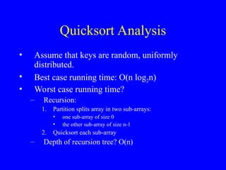
60. Quicksort Analysis • Assume that keys are random, uniformly distributed. • Best case running time: O(n log2n) • Worst case running time? – Recursion: 1. Partition splits array in two sub-arrays: • one sub-array of size 0 • the other sub-array of size n-1 2. Quicksort each sub-array – Depth of recursion tree?

61. Quicksort Analysis • Assume that keys are random, uniformly distributed. • Best case running time: O(n log2n) • Worst case running time? – Recursion: 1. Partition splits array in two sub-arrays: • one sub-array of size 0 • the other sub-array of size n-1 2. Quicksort each sub-array – Depth of recursion tree? O(n)

62. Quicksort Analysis • Assume that keys are random, uniformly distributed. • Best case running time: O(n log2n) • Worst case running time? – Recursion: 1. Partition splits array in two sub-arrays: • one sub-array of size 0 • the other sub-array of size n-1 2. Quicksort each sub-array – Depth of recursion tree? O(n) – Number of accesses per partition?

63. Quicksort Analysis • Assume that keys are random, uniformly distributed. • Best case running time: O(n log2n) • Worst case running time? – Recursion: 1. Partition splits array in two sub-arrays: • one sub-array of size 0 • the other sub-array of size n-1 2. Quicksort each sub-array – Depth of recursion tree? O(n) – Number of accesses per partition? O(n)

64. Quicksort Analysis • Assume that keys are random, uniformly distributed. • Best case running time: O(n log2n) • Worst case running time: O(n2 )!!!

65. Quicksort Analysis • Assume that keys are random, uniformly distributed. • Best case running time: O(n log2n) • Worst case running time: O(n2 )!!! • What can we do to avoid worst case?

66. Improved Pivot Selection Pick median value of three elements from data array: data[0], data[n/2], and data[n-1]. Use this median value as pivot.

67. Improving Performance of Quicksort • Improved selection of pivot. • For sub-arrays of size 3 or less, apply brute force search: – Sub-array of size 1: trivial – Sub-array of size 2: • if(data[first] > data[second]) swap them – Sub-array of size 3: left as an exercise.

Quicksort and MergeSort Algorithm Analysis

Recommended

More Related Content

Similar to Quicksort and MergeSort Algorithm Analysis (20)

Recently uploaded (20)

Quicksort and MergeSort Algorithm Analysis