SlideShare a Scribd company logo
Regression Analysis
• Regression analysis is used in statistics to find trends in
data.
For example, you might guess that there’s a connection
between how much you eat and how much you weigh.
• In statistical modelling, regression analysis is a set of
statistical procedures for estimating the relationships
between a dependent variable(outcome: weight) and
one or more independent variable(predictors,
covariates, features: amount of food we eat).
• It provides an equation for a graph so that you can make
predictions about your data.
Regression Analysis Example
Year vs RainFall Record
Formula can be represented as y=mx+b
Regression gives you a useful equation, which for this chart
is:
y = -2.2923x + 4624.4
• Best of all, you can use the equation to make predictions.
For example, how much snow will fall in 2017?
y = -2.2923(2017) + 4624.4 = 0.8 inches.
• Regression also gives you an R2
value, which for this graph
is 0.702. This number tells you how good your model is.
• The values range from 0 to 1, with 0 being a terrible model
and 1 being a perfect model. As you can probably see, 0.7
is a fairly decent model so you can be fairly confident in your
weather prediction!
There are multiple benefits of using regression analysis:
• It indicates the significant relationships between dependent variable
and independent variable.
• It indicates the strength of impact of multiple independent variables
on a dependent variable.
In Regression analysis, we fit a curve / line to the data
points, in such a manner that the differences between the
distances of data points from the curve or line is minimized.
Regression Analysis
These techniques are mostly driven by three metrics (number
of independent variables, type of dependent variables and
shape of regression line).
Regression Techniques
•Simple Linear regression(Univariate) analysis
uses a single x variable for each dependent “y”
variable. For example: (x, Y).
•Multiple Linear regression(Multivariate) uses
multiple “x” variables for each independent
variable: (x1)1, (x2)1, (x3)1, Y1).
•Nonlinear Regression if the regression curve is
nonlinear then there is nonlinear regression
between variables
Regression Techniques
Regression Types
1.Simple and Multiple Linear Regression
2.Logistic Regression
3.Polynomial Regression
4.Ridge Regression and Lasso Regression (upgrades to Linear
Regression)
Linear Regression
• Dependent variable is continuous
• Independent variable(s) can be continuous or discrete
• Nature of regression line is linear.
• It establishes a relationship between dependent variable (Y) and one or
more independent variables (X) using a best fit straight line (also known
as regression line).
• Equation Y=m*X + c + e, where ‘c’ is intercept, ‘m’ is slope of the line and ’e’
is error term.
How to obtain best fit line (Value of m and c)?
• Least Square Method: A most common method used for fitting a
regression line.
• It calculates the best-fit line for the observed data by minimizing the sum of
the squares of the vertical deviations from each data point to the line.
• Error is the difference between the actual value and Predicted value and
the goal is to reduce this difference.
How to obtain best fit line (Value of m and c)?
• The vertical distance between the data point and the regression line is
known as Error or Residual.
• Each data point has one residual and the sum of all the differences is
known as the Sum of Residuals/Errors.
How to obtain best fit line (Value of m and c)?
Residual/Error = Actual values – Predicted Values
Sum of Residuals/Errors = Sum(Actual- Predicted Values)
Square of Sum of Residuals/Errors = (Sum(Actual- Predicted Values))2
Aim is to minimize this sum of square error term or Cost Fuction
Least Square Method / Ordinary Least Square (OLS):
For equation: y = mx + b
Use the least square method to determine the equation of line of best fit for
the data. Then plot the line.
regression analysis presentation slides.
Metrix(s) for Model Evaluation
• Residual Sum of Squares (RSS). Sum of difference between
each actual output and the predicted output.
• Mean Square Error (MSE) is computed as RSS divided by the
total number of data points.
• Root Mean Squared Error (RMSE)
Metrix(s) for Model Evaluation
• R-squared is the proportion of the variance in the dependent
variable that is predicted from the independent variable.
• It ranges from 0 to 1.
• With linear regression, the coefficient of determination is equal
to the square of the correlation between the x and y variables.
• If R2 is equal to 0, then the dependent variable cannot be
predicted from the independent variable.
• If R2 is equal to 1, then the dependent variable can be predicted
from the independent variable without any error.
Metrix(s) for Model Evaluation
R-squared:
Formula 1: Using correlation coefficient
Formula 2: Using sum of squares.
Square this value to get the coefficient of determination
Example:
• Last year, five randomly selected students took a math aptitude test before
they began their statistics course. The Statistics Department has three
questions:
• What linear regression equation best predicts statistics performance,
based on math aptitude scores?
• If a student made an 80 on the aptitude test, what grade would we expect
her to make in statistics?
• How well does the regression equation fit the data?
x 95 85 80 70 60
y 85 95 70 65 70
What linear regression equation best predicts statistics performance, based on math aptitude scores?
If a student made an 80 on the aptitude test, what grade would we expect her to make in statistics?
How well does the regression equation fit the data?
regression analysis presentation slides.
What linear regression equation best predicts statistics performance, based on math aptitude scores?
If a student made an 80 on the aptitude test, what grade would we expect her to make in statistics?
How well does the regression equation fit the data?
What linear regression equation best predicts statistics performance, based on math aptitude scores?
If a student made an 80 on the aptitude test, what grade would we expect her to make in statistics?
How well does the regression equation fit the data?
Calculate the Value of R2
Linear Regression: Assumptions
• Linearity: the dependent variable Y should be linearly related
to independent variables.
• Normality: The X and Y variables should be normally distributed
• Homoscedasticity: The variance of the error terms should be
constant
• Independence/No Multicollinearity: No correlation should be
there between the independent variables.
• The error terms should be normally distributed
• No Autocorrelation: The error terms should be independent of
each other.
Cost Function
• The whole idea of the linear Regression is to find the best fit
line, which has very low error (cost function).
Properties of the Regression line:
• 1. The line minimizes the sum of squared difference between the
observed values(actual y-value) and the predicted value(ŷ value)
• 2. The line passes through the mean of independent and dependent
features.
Cost Function vs Loss Function
• The loss function calculates the error per observation,
whilst the cost function calculates the error over the whole
dataset.
Linear Regression: Gradient Descent
• Gradient descent is an optimization algorithm used to find the
values of parameters (coefficients) of a function that minimizes
a cost function (cost).
• The idea is to start with random m and b values and then
iteratively updating the values, reaching minimum cost.
• Steps:
1. Initially, the values of m and b will be 0 and the learning rate(α) will be
introduced to the function. The value of learning rate(α) is taken very
small, something between 0.01 or 0.0001.
The learning rate is a tuning parameter in an optimization algorithm that determines the
step size at each iteration while moving toward a minimum of a cost function.
Linear Regression: Gradient Descent
2. Partial derivative is calculate for the cost function equation in terms of
slope(m) and also derivatives are calculated with respect to the intercept(b)
3. After the derivatives are calculated, The slope(m) and intercept(b) are updated with
the help of the following equation.
m = m-α*derivative of m
b = b-α*derivative of b
4. The process of updating the values of m and b continues until the cost function
reaches the ideal value of 0 or close to 0.
Multiple Linear Regression
• The main difference is the number of independent variables
that they take as inputs. Simple linear regression just takes a
single feature, while multiple linear regression takes
multiple x values.
• Another way is to use Normal Equation with multiple
independent variables.
Multiple Linear Regression
• The main difference is the number of independent variables
that they take as inputs. Simple linear regression just takes a
single feature, while multiple linear regression takes
multiple x values.
ŷ = b0 + b1x1 + b2x2 + … + bk-1xk-1 + bkxk
Y = Xb
b = (X'X)-1
X'Y
Multiple Linear Regression: Example
Student Test score IQ Study hours
1 100 110 40
2 90 120 30
3 80 100 20
4 70 90 0
5 60 80 10
Multiple Linear Regression: Example
•Define X.
•Define X'.
•Compute X'X.
•Find the inverse of X'X.
•Define Y.
Multiple Linear Regression: Example
b = (X'X)-1
X'Y
ŷ = 20 + 0.5x1 +0.5x2
Regression Types
1.Simple and Multiple Linear Regression
2.Logistic Regression
3.Polynomial Regression
4.Ridge Regression and Lasso Regression (upgrades to
Linear Regression)
5.Decision Trees Regression
6.Support Vector Regression (SVR)
Logistic Regression
• Logistic Regression is used when the dependent variable(target) is
categorical or binary. For example:
• To predict whether an email is spam (1) or (0)
• Whether the tumor is malignant (1) or not (0)
• Logistic regression is widely used for classification problems
• Logistic regression doesn’t require linear relationship between
dependent and independent variables.
• Logistic regression estimates the probability of an event belonging to
a class, such as voted or didn’t vote.
HR Analytics : IT firms recruit large number of people, but
one of the problems they encounter is after accepting the job
offer many candidates do not join. So, this results in cost
over-runs because they have to repeat the entire process
again. Now when you get an application, can you actually
predict whether that applicant is likely to join the organization
(Binary Outcome - Join / Not Join).
Logistic Regression Example
Why Logistic Regression
In Linear regression, we draw a straight line(the best fit line) L1 such that the sum of distances
of all the data points to the line is minimal.
It uses sigmoid function is to map any predicted values of
probabilities into another value between 0 and 1.
Logistic Regression Equation
Linear model: ŷ = b0+b1x
Sigmoid function: σ(z) = 1/(1+e z
−
)
Logistic regression model:
ŷ = σ(b0+b1x) = 1/(1+e-(b0+b1x)
)
Also called logistic or logit function
Logistic Regression Equation
To make in the range from 0 to +infinity
To make in the range from -infinity to +infinity
Since we want to calculate value of p
In logistic regression, as the output is a probability value between
0 or 1, mean squared error wouldn’t be the right choice. Instead,
we use the log loss function which is derived from the maximum
likelihood estimation method.
Logistic Regression Evaluation
Overfitting and Underfitting
Derive
Hypothesis
Bias
• Bias is simply defined as the inability of the model because of
that there is some difference or error occurring between the
model’s predicted value and the actual value. These differences
between actual or expected values and the predicted values are
known as error or bias error or error due to bias.
• Let Y be the true value of a parameter, and let Y^ be an estimator
of Y based on a sample of data. Then, the bias of the
estimator Y^ is given by:
• Bias(Y^)=E(Y^)–Y
• where E(Y^) is the expected value of the estimator Y. It is the
measurement of the model that how well it fits the data.
Bias
• Low Bias: Low bias value means fewer assumptions are
taken to build the target function. In this case, the
model will closely match the training dataset.
• High Bias: High bias value means more assumptions are
taken to build the target function. In this case, the model
will not match the training dataset closely.
• The high-bias model will not be able to capture the dataset
trend. It is considered as the underfitting model which has
a high error rate. It is due to a very simplified algorithm.
Variance
• The variance is the variability of the model that how much it is
sensitive to another subset of the training dataset. i.e. how much it
can adjust on the new subset of the training dataset.
• Let Y be the actual values of the target variable, and Y^ be the
predicted values of the target variable.
• Then the variance of a model can be measured as the expected value
of the square of the difference between predicted values and the
expected value of the predicted values.
• Variance=E[(Y^–E[Y^])2]
• where E[Yˉ]E[Yˉ] is the expected value of the predicted values. Here expected value is
averaged over all the training data.
• Variance errors are either low or high-variance errors.
• Low variance: Low variance means that the model is less sensitive to changes in the
training data and can produce consistent estimates of the target function with
different subsets of data from the same distribution. This is the case of underfitting
when the model fails to generalize on both training and test data.
• High variance: High variance means that the model is very sensitive to changes in
the training data and can result in significant changes in the estimate of the target
function when trained on different subsets of data from the same distribution. This
is the case of overfitting when the model performs well on the training data but
poorly on new, unseen test data. It fits the training data too closely that it fails on the
new training dataset.
Overfitting and Underfitting
Underfitting is a situation when your model is too simple for
your data or your hypothesis about data distribution is wrong
and too simple. For example, your data is quadratic, and your
model is linear.
This situation is also called high bias.
This means that your algorithm can do
accurate predictions, but the initial
assumption about the data is incorrect.
Overfitting and Underfitting
Overfitting is a situation when your model is too complex for your
data.
For example, your data is linear and your model is high-
degree polynomial.
This situation is also called high variance.
In this situation, changing the input data only a little, the
model output changes very much.
•low bias, low variance — is a good result, just right.
•low bias, high variance — overfitting — the algorithm outputs very different
predictions for similar data.
•high bias, low variance — underfitting — the algorithm outputs similar predictions
for similar data, but predictions are wrong (algorithm “miss”).
•high bias, high variance — very bad algorithm. You will most likely never see this.
Overfitting
and
Underfitting
Regularization
• Regularization is one of the ways to improve our model to
work on unseen data by ignoring the less important
features.
• Regularization minimizes the validation loss and tries to
improve the accuracy of the model.
• It avoids overfitting by adding a penalty to the model with
high variance.
LASSO stands for Least Absolute Shrinkage and Selection
Operator.
Lasso regression performs L1 regularization, i.e. it adds a factor
of sum of absolute value of coefficients in the optimization
objective.
This type of regularization (L1) can lead to zero coefficients i.e.
some of the features are completely neglected for the evaluation
of output. So, Lasso regression not only helps in reducing over-
Lasso Regression
In ridge regression, the cost function is altered by adding a
penalty equivalent to square of the magnitude of the coefficients.
The penalty term (lambda) regularizes the coefficients such that if the
coefficients take large values the optimization function is penalized.
Ridge regression shrinks the coefficients and it helps to reduce the model
complexity and multi-collinearity
It is also called “L2 regularization”.
Ridge Regression
Polynomial Regression
• A regression equation is a polynomial regression equation if
the power of independent variable is more than 1. The
equation below represents a polynomial equation:
• In this regression technique, the best fit line is not a straight
line. It is rather a curve that fits into the data points.
Lasso vs Ridge
Regression vs Classification
• Classification predictions can be evaluated using accuracy,
whereas regression predictions cannot.
• Regression predictions can be evaluated using root mean
squared error, whereas classification predictions cannot.
• A classification algorithm may predict a continuous value,
but the continuous value is in the form of a probability for a
class label.
• A regression algorithm may predict a discrete value, but the
discrete value in the form of an integer quantity.
Ad

More Related Content

Similar to regression analysis presentation slides. (20)

Simple lin regress_inference
Simple lin regress_inferenceSimple lin regress_inference
Simple lin regress_inference
Kemal İnciroğlu
 
Unit-III Correlation and Regression.pptx
Unit-III Correlation and Regression.pptxUnit-III Correlation and Regression.pptx
Unit-III Correlation and Regression.pptx
Anusuya123
 
The normal presentation about linear regression in machine learning
The normal presentation about linear regression in machine learningThe normal presentation about linear regression in machine learning
The normal presentation about linear regression in machine learning
dawasthi952
 
Forecasting Using the Predictive Analytics
Forecasting Using the Predictive AnalyticsForecasting Using the Predictive Analytics
Forecasting Using the Predictive Analytics
PRPrasad1
 
Statr session 23 and 24
Statr session 23 and 24Statr session 23 and 24
Statr session 23 and 24
Ruru Chowdhury
 
2a-linear-regression-18Maykjkij;oik;.pptx
2a-linear-regression-18Maykjkij;oik;.pptx2a-linear-regression-18Maykjkij;oik;.pptx
2a-linear-regression-18Maykjkij;oik;.pptx
rundalomary12
 
probability distribution term 1 IMI New Delhi.pdf
probability distribution term 1 IMI New Delhi.pdfprobability distribution term 1 IMI New Delhi.pdf
probability distribution term 1 IMI New Delhi.pdf
iabhimanyusingh1
 
probability distribution term 1 IMI New Delhi.pdf
probability distribution term 1 IMI New Delhi.pdfprobability distribution term 1 IMI New Delhi.pdf
probability distribution term 1 IMI New Delhi.pdf
iabhimanyusingh1
 
Lecture 5 - Linear Regression Linear Regression
Lecture 5 - Linear Regression Linear RegressionLecture 5 - Linear Regression Linear Regression
Lecture 5 - Linear Regression Linear Regression
viyah59114
 
Data analytics Lecture power point presentations
Data analytics Lecture power point presentationsData analytics Lecture power point presentations
Data analytics Lecture power point presentations
sharmahemant3612
 
11Polynomial RegressionPolynomial RegressionPolynomial RegressionPolynomial R...
11Polynomial RegressionPolynomial RegressionPolynomial RegressionPolynomial R...11Polynomial RegressionPolynomial RegressionPolynomial RegressionPolynomial R...
11Polynomial RegressionPolynomial RegressionPolynomial RegressionPolynomial R...
FaizaKhan720183
 
numerical method chapter 5.pptxggggvvgggbg
numerical method chapter 5.pptxggggvvgggbgnumerical method chapter 5.pptxggggvvgggbg
numerical method chapter 5.pptxggggvvgggbg
Natinael10
 
Regression Analysis.pptx
Regression Analysis.pptxRegression Analysis.pptx
Regression Analysis.pptx
ShivankAggatwal
 
Regression vs Neural Net
Regression vs Neural NetRegression vs Neural Net
Regression vs Neural Net
Ratul Alahy
 
Simple egression.pptx
Simple egression.pptxSimple egression.pptx
Simple egression.pptx
AbdalrahmanTahaJaya
 
Simple Linear Regression.pptx
Simple Linear Regression.pptxSimple Linear Regression.pptx
Simple Linear Regression.pptx
AbdalrahmanTahaJaya
 
Linear regression
Linear regressionLinear regression
Linear regression
MartinHogg9
 
Regression analysis ppt
Regression analysis pptRegression analysis ppt
Regression analysis ppt
Elkana Rorio
 
Linear Regression
Linear RegressionLinear Regression
Linear Regression
Abdullah al Mamun
 
Simple & Multiple Regression Analysis
Simple & Multiple Regression AnalysisSimple & Multiple Regression Analysis
Simple & Multiple Regression Analysis
Shailendra Tomar
 
Simple lin regress_inference
Simple lin regress_inferenceSimple lin regress_inference
Simple lin regress_inference
Kemal İnciroğlu
 
Unit-III Correlation and Regression.pptx
Unit-III Correlation and Regression.pptxUnit-III Correlation and Regression.pptx
Unit-III Correlation and Regression.pptx
Anusuya123
 
The normal presentation about linear regression in machine learning
The normal presentation about linear regression in machine learningThe normal presentation about linear regression in machine learning
The normal presentation about linear regression in machine learning
dawasthi952
 
Forecasting Using the Predictive Analytics
Forecasting Using the Predictive AnalyticsForecasting Using the Predictive Analytics
Forecasting Using the Predictive Analytics
PRPrasad1
 
Statr session 23 and 24
Statr session 23 and 24Statr session 23 and 24
Statr session 23 and 24
Ruru Chowdhury
 
2a-linear-regression-18Maykjkij;oik;.pptx
2a-linear-regression-18Maykjkij;oik;.pptx2a-linear-regression-18Maykjkij;oik;.pptx
2a-linear-regression-18Maykjkij;oik;.pptx
rundalomary12
 
probability distribution term 1 IMI New Delhi.pdf
probability distribution term 1 IMI New Delhi.pdfprobability distribution term 1 IMI New Delhi.pdf
probability distribution term 1 IMI New Delhi.pdf
iabhimanyusingh1
 
probability distribution term 1 IMI New Delhi.pdf
probability distribution term 1 IMI New Delhi.pdfprobability distribution term 1 IMI New Delhi.pdf
probability distribution term 1 IMI New Delhi.pdf
iabhimanyusingh1
 
Lecture 5 - Linear Regression Linear Regression
Lecture 5 - Linear Regression Linear RegressionLecture 5 - Linear Regression Linear Regression
Lecture 5 - Linear Regression Linear Regression
viyah59114
 
Data analytics Lecture power point presentations
Data analytics Lecture power point presentationsData analytics Lecture power point presentations
Data analytics Lecture power point presentations
sharmahemant3612
 
11Polynomial RegressionPolynomial RegressionPolynomial RegressionPolynomial R...
11Polynomial RegressionPolynomial RegressionPolynomial RegressionPolynomial R...11Polynomial RegressionPolynomial RegressionPolynomial RegressionPolynomial R...
11Polynomial RegressionPolynomial RegressionPolynomial RegressionPolynomial R...
FaizaKhan720183
 
numerical method chapter 5.pptxggggvvgggbg
numerical method chapter 5.pptxggggvvgggbgnumerical method chapter 5.pptxggggvvgggbg
numerical method chapter 5.pptxggggvvgggbg
Natinael10
 
Regression Analysis.pptx
Regression Analysis.pptxRegression Analysis.pptx
Regression Analysis.pptx
ShivankAggatwal
 
Regression vs Neural Net
Regression vs Neural NetRegression vs Neural Net
Regression vs Neural Net
Ratul Alahy
 
Linear regression
Linear regressionLinear regression
Linear regression
MartinHogg9
 
Regression analysis ppt
Regression analysis pptRegression analysis ppt
Regression analysis ppt
Elkana Rorio
 
Simple & Multiple Regression Analysis
Simple & Multiple Regression AnalysisSimple & Multiple Regression Analysis
Simple & Multiple Regression Analysis
Shailendra Tomar
 

Recently uploaded (20)

Storage Devices and the Mechanism of Data Storage in Audio and Visual Form
Storage Devices and the Mechanism of Data Storage in Audio and Visual FormStorage Devices and the Mechanism of Data Storage in Audio and Visual Form
Storage Devices and the Mechanism of Data Storage in Audio and Visual Form
Professional Content Writing's
 
Dr. Robert Krug - Expert In Artificial Intelligence
Dr. Robert Krug - Expert In Artificial IntelligenceDr. Robert Krug - Expert In Artificial Intelligence
Dr. Robert Krug - Expert In Artificial Intelligence
Dr. Robert Krug
 
Day 1 MS Excel Basics #.pptxDay 1 MS Excel Basics #.pptxDay 1 MS Excel Basics...
Day 1 MS Excel Basics #.pptxDay 1 MS Excel Basics #.pptxDay 1 MS Excel Basics...Day 1 MS Excel Basics #.pptxDay 1 MS Excel Basics #.pptxDay 1 MS Excel Basics...
Day 1 MS Excel Basics #.pptxDay 1 MS Excel Basics #.pptxDay 1 MS Excel Basics...
Jayantilal Bhanushali
 
Carbon Nanomaterials Market Size, Trends and Outlook 2024-2030
Carbon Nanomaterials Market Size, Trends and Outlook 2024-2030Carbon Nanomaterials Market Size, Trends and Outlook 2024-2030
Carbon Nanomaterials Market Size, Trends and Outlook 2024-2030
Industry Experts
 
presentacion.slideshare.informáticaJuridica..pptx
presentacion.slideshare.informáticaJuridica..pptxpresentacion.slideshare.informáticaJuridica..pptx
presentacion.slideshare.informáticaJuridica..pptx
GersonVillatoro4
 
What is ETL? Difference between ETL and ELT?.pdf
What is ETL? Difference between ETL and ELT?.pdfWhat is ETL? Difference between ETL and ELT?.pdf
What is ETL? Difference between ETL and ELT?.pdf
SaikatBasu37
 
Lesson-2.pptxjsjahajauahahagqiqhwjwjahaiq
Lesson-2.pptxjsjahajauahahagqiqhwjwjahaiqLesson-2.pptxjsjahajauahahagqiqhwjwjahaiq
Lesson-2.pptxjsjahajauahahagqiqhwjwjahaiq
AngelPinedaTaguinod
 
Publication-launch-How-is-Life-for-Children-in-the-Digital-Age-15-May-2025.pdf
Publication-launch-How-is-Life-for-Children-in-the-Digital-Age-15-May-2025.pdfPublication-launch-How-is-Life-for-Children-in-the-Digital-Age-15-May-2025.pdf
Publication-launch-How-is-Life-for-Children-in-the-Digital-Age-15-May-2025.pdf
StatsCommunications
 
national income & related aggregates (1)(1).pptx
national income & related aggregates (1)(1).pptxnational income & related aggregates (1)(1).pptx
national income & related aggregates (1)(1).pptx
j2492618
 
Lesson 6-Interviewing in SHRM_updated.pdf
Lesson 6-Interviewing in SHRM_updated.pdfLesson 6-Interviewing in SHRM_updated.pdf
Lesson 6-Interviewing in SHRM_updated.pdf
hemelali11
 
Important JavaScript Concepts Every Developer Must Know
Important JavaScript Concepts Every Developer Must KnowImportant JavaScript Concepts Every Developer Must Know
Important JavaScript Concepts Every Developer Must Know
yashikanigam1
 
Time series analysis & forecasting day 2.pptx
Time series analysis & forecasting day 2.pptxTime series analysis & forecasting day 2.pptx
Time series analysis & forecasting day 2.pptx
AsmaaMahmoud89
 
web-roadmap developer file information..
web-roadmap developer file information..web-roadmap developer file information..
web-roadmap developer file information..
pandeyarush01
 
Urban models for professional practice 03
Urban models for professional practice 03Urban models for professional practice 03
Urban models for professional practice 03
DanisseLoiDapdap
 
report (maam dona subject).pptxhsgwiswhs
report (maam dona subject).pptxhsgwiswhsreport (maam dona subject).pptxhsgwiswhs
report (maam dona subject).pptxhsgwiswhs
AngelPinedaTaguinod
 
最新版澳洲西澳大利亚大学毕业证(UWA毕业证书)原版定制
最新版澳洲西澳大利亚大学毕业证(UWA毕业证书)原版定制最新版澳洲西澳大利亚大学毕业证(UWA毕业证书)原版定制
最新版澳洲西澳大利亚大学毕业证(UWA毕业证书)原版定制
Taqyea
 
Introduction to systems thinking tools_Eng.pdf
Introduction to systems thinking tools_Eng.pdfIntroduction to systems thinking tools_Eng.pdf
Introduction to systems thinking tools_Eng.pdf
AbdurahmanAbd
 
Digital Disruption Use Case_Music Industry_for students.pdf
Digital Disruption Use Case_Music Industry_for students.pdfDigital Disruption Use Case_Music Industry_for students.pdf
Digital Disruption Use Case_Music Industry_for students.pdf
ProsenjitMitra9
 
英国学位证(利物浦约翰摩尔斯大学本科毕业证)LJMU文凭证书办理
英国学位证(利物浦约翰摩尔斯大学本科毕业证)LJMU文凭证书办理英国学位证(利物浦约翰摩尔斯大学本科毕业证)LJMU文凭证书办理
英国学位证(利物浦约翰摩尔斯大学本科毕业证)LJMU文凭证书办理
Taqyea
 
Get Started with FukreyGame Today!......
Get Started with FukreyGame Today!......Get Started with FukreyGame Today!......
Get Started with FukreyGame Today!......
liononline785
 
Storage Devices and the Mechanism of Data Storage in Audio and Visual Form
Storage Devices and the Mechanism of Data Storage in Audio and Visual FormStorage Devices and the Mechanism of Data Storage in Audio and Visual Form
Storage Devices and the Mechanism of Data Storage in Audio and Visual Form
Professional Content Writing's
 
Dr. Robert Krug - Expert In Artificial Intelligence
Dr. Robert Krug - Expert In Artificial IntelligenceDr. Robert Krug - Expert In Artificial Intelligence
Dr. Robert Krug - Expert In Artificial Intelligence
Dr. Robert Krug
 
Day 1 MS Excel Basics #.pptxDay 1 MS Excel Basics #.pptxDay 1 MS Excel Basics...
Day 1 MS Excel Basics #.pptxDay 1 MS Excel Basics #.pptxDay 1 MS Excel Basics...Day 1 MS Excel Basics #.pptxDay 1 MS Excel Basics #.pptxDay 1 MS Excel Basics...
Day 1 MS Excel Basics #.pptxDay 1 MS Excel Basics #.pptxDay 1 MS Excel Basics...
Jayantilal Bhanushali
 
Carbon Nanomaterials Market Size, Trends and Outlook 2024-2030
Carbon Nanomaterials Market Size, Trends and Outlook 2024-2030Carbon Nanomaterials Market Size, Trends and Outlook 2024-2030
Carbon Nanomaterials Market Size, Trends and Outlook 2024-2030
Industry Experts
 
presentacion.slideshare.informáticaJuridica..pptx
presentacion.slideshare.informáticaJuridica..pptxpresentacion.slideshare.informáticaJuridica..pptx
presentacion.slideshare.informáticaJuridica..pptx
GersonVillatoro4
 
What is ETL? Difference between ETL and ELT?.pdf
What is ETL? Difference between ETL and ELT?.pdfWhat is ETL? Difference between ETL and ELT?.pdf
What is ETL? Difference between ETL and ELT?.pdf
SaikatBasu37
 
Lesson-2.pptxjsjahajauahahagqiqhwjwjahaiq
Lesson-2.pptxjsjahajauahahagqiqhwjwjahaiqLesson-2.pptxjsjahajauahahagqiqhwjwjahaiq
Lesson-2.pptxjsjahajauahahagqiqhwjwjahaiq
AngelPinedaTaguinod
 
Publication-launch-How-is-Life-for-Children-in-the-Digital-Age-15-May-2025.pdf
Publication-launch-How-is-Life-for-Children-in-the-Digital-Age-15-May-2025.pdfPublication-launch-How-is-Life-for-Children-in-the-Digital-Age-15-May-2025.pdf
Publication-launch-How-is-Life-for-Children-in-the-Digital-Age-15-May-2025.pdf
StatsCommunications
 
national income & related aggregates (1)(1).pptx
national income & related aggregates (1)(1).pptxnational income & related aggregates (1)(1).pptx
national income & related aggregates (1)(1).pptx
j2492618
 
Lesson 6-Interviewing in SHRM_updated.pdf
Lesson 6-Interviewing in SHRM_updated.pdfLesson 6-Interviewing in SHRM_updated.pdf
Lesson 6-Interviewing in SHRM_updated.pdf
hemelali11
 
Important JavaScript Concepts Every Developer Must Know
Important JavaScript Concepts Every Developer Must KnowImportant JavaScript Concepts Every Developer Must Know
Important JavaScript Concepts Every Developer Must Know
yashikanigam1
 
Time series analysis & forecasting day 2.pptx
Time series analysis & forecasting day 2.pptxTime series analysis & forecasting day 2.pptx
Time series analysis & forecasting day 2.pptx
AsmaaMahmoud89
 
web-roadmap developer file information..
web-roadmap developer file information..web-roadmap developer file information..
web-roadmap developer file information..
pandeyarush01
 
Urban models for professional practice 03
Urban models for professional practice 03Urban models for professional practice 03
Urban models for professional practice 03
DanisseLoiDapdap
 
report (maam dona subject).pptxhsgwiswhs
report (maam dona subject).pptxhsgwiswhsreport (maam dona subject).pptxhsgwiswhs
report (maam dona subject).pptxhsgwiswhs
AngelPinedaTaguinod
 
最新版澳洲西澳大利亚大学毕业证(UWA毕业证书)原版定制
最新版澳洲西澳大利亚大学毕业证(UWA毕业证书)原版定制最新版澳洲西澳大利亚大学毕业证(UWA毕业证书)原版定制
最新版澳洲西澳大利亚大学毕业证(UWA毕业证书)原版定制
Taqyea
 
Introduction to systems thinking tools_Eng.pdf
Introduction to systems thinking tools_Eng.pdfIntroduction to systems thinking tools_Eng.pdf
Introduction to systems thinking tools_Eng.pdf
AbdurahmanAbd
 
Digital Disruption Use Case_Music Industry_for students.pdf
Digital Disruption Use Case_Music Industry_for students.pdfDigital Disruption Use Case_Music Industry_for students.pdf
Digital Disruption Use Case_Music Industry_for students.pdf
ProsenjitMitra9
 
英国学位证(利物浦约翰摩尔斯大学本科毕业证)LJMU文凭证书办理
英国学位证(利物浦约翰摩尔斯大学本科毕业证)LJMU文凭证书办理英国学位证(利物浦约翰摩尔斯大学本科毕业证)LJMU文凭证书办理
英国学位证(利物浦约翰摩尔斯大学本科毕业证)LJMU文凭证书办理
Taqyea
 
Get Started with FukreyGame Today!......
Get Started with FukreyGame Today!......Get Started with FukreyGame Today!......
Get Started with FukreyGame Today!......
liononline785
 
Ad

regression analysis presentation slides.

  • 1. Regression Analysis • Regression analysis is used in statistics to find trends in data. For example, you might guess that there’s a connection between how much you eat and how much you weigh. • In statistical modelling, regression analysis is a set of statistical procedures for estimating the relationships between a dependent variable(outcome: weight) and one or more independent variable(predictors, covariates, features: amount of food we eat). • It provides an equation for a graph so that you can make predictions about your data.
  • 2. Regression Analysis Example Year vs RainFall Record Formula can be represented as y=mx+b
  • 3. Regression gives you a useful equation, which for this chart is: y = -2.2923x + 4624.4 • Best of all, you can use the equation to make predictions. For example, how much snow will fall in 2017? y = -2.2923(2017) + 4624.4 = 0.8 inches. • Regression also gives you an R2 value, which for this graph is 0.702. This number tells you how good your model is. • The values range from 0 to 1, with 0 being a terrible model and 1 being a perfect model. As you can probably see, 0.7 is a fairly decent model so you can be fairly confident in your weather prediction!
  • 4. There are multiple benefits of using regression analysis: • It indicates the significant relationships between dependent variable and independent variable. • It indicates the strength of impact of multiple independent variables on a dependent variable. In Regression analysis, we fit a curve / line to the data points, in such a manner that the differences between the distances of data points from the curve or line is minimized. Regression Analysis
  • 5. These techniques are mostly driven by three metrics (number of independent variables, type of dependent variables and shape of regression line). Regression Techniques
  • 6. •Simple Linear regression(Univariate) analysis uses a single x variable for each dependent “y” variable. For example: (x, Y). •Multiple Linear regression(Multivariate) uses multiple “x” variables for each independent variable: (x1)1, (x2)1, (x3)1, Y1). •Nonlinear Regression if the regression curve is nonlinear then there is nonlinear regression between variables Regression Techniques
  • 7. Regression Types 1.Simple and Multiple Linear Regression 2.Logistic Regression 3.Polynomial Regression 4.Ridge Regression and Lasso Regression (upgrades to Linear Regression)
  • 8. Linear Regression • Dependent variable is continuous • Independent variable(s) can be continuous or discrete • Nature of regression line is linear. • It establishes a relationship between dependent variable (Y) and one or more independent variables (X) using a best fit straight line (also known as regression line). • Equation Y=m*X + c + e, where ‘c’ is intercept, ‘m’ is slope of the line and ’e’ is error term.
  • 9. How to obtain best fit line (Value of m and c)? • Least Square Method: A most common method used for fitting a regression line. • It calculates the best-fit line for the observed data by minimizing the sum of the squares of the vertical deviations from each data point to the line. • Error is the difference between the actual value and Predicted value and the goal is to reduce this difference.
  • 10. How to obtain best fit line (Value of m and c)? • The vertical distance between the data point and the regression line is known as Error or Residual. • Each data point has one residual and the sum of all the differences is known as the Sum of Residuals/Errors.
  • 11. How to obtain best fit line (Value of m and c)? Residual/Error = Actual values – Predicted Values Sum of Residuals/Errors = Sum(Actual- Predicted Values) Square of Sum of Residuals/Errors = (Sum(Actual- Predicted Values))2 Aim is to minimize this sum of square error term or Cost Fuction
  • 12. Least Square Method / Ordinary Least Square (OLS): For equation: y = mx + b
  • 13. Use the least square method to determine the equation of line of best fit for the data. Then plot the line.
  • 15. Metrix(s) for Model Evaluation • Residual Sum of Squares (RSS). Sum of difference between each actual output and the predicted output. • Mean Square Error (MSE) is computed as RSS divided by the total number of data points. • Root Mean Squared Error (RMSE)
  • 16. Metrix(s) for Model Evaluation • R-squared is the proportion of the variance in the dependent variable that is predicted from the independent variable. • It ranges from 0 to 1. • With linear regression, the coefficient of determination is equal to the square of the correlation between the x and y variables. • If R2 is equal to 0, then the dependent variable cannot be predicted from the independent variable. • If R2 is equal to 1, then the dependent variable can be predicted from the independent variable without any error.
  • 17. Metrix(s) for Model Evaluation R-squared: Formula 1: Using correlation coefficient Formula 2: Using sum of squares. Square this value to get the coefficient of determination
  • 18. Example: • Last year, five randomly selected students took a math aptitude test before they began their statistics course. The Statistics Department has three questions: • What linear regression equation best predicts statistics performance, based on math aptitude scores? • If a student made an 80 on the aptitude test, what grade would we expect her to make in statistics? • How well does the regression equation fit the data? x 95 85 80 70 60 y 85 95 70 65 70
  • 19. What linear regression equation best predicts statistics performance, based on math aptitude scores? If a student made an 80 on the aptitude test, what grade would we expect her to make in statistics? How well does the regression equation fit the data?
  • 21. What linear regression equation best predicts statistics performance, based on math aptitude scores? If a student made an 80 on the aptitude test, what grade would we expect her to make in statistics? How well does the regression equation fit the data?
  • 22. What linear regression equation best predicts statistics performance, based on math aptitude scores? If a student made an 80 on the aptitude test, what grade would we expect her to make in statistics? How well does the regression equation fit the data? Calculate the Value of R2
  • 23. Linear Regression: Assumptions • Linearity: the dependent variable Y should be linearly related to independent variables. • Normality: The X and Y variables should be normally distributed • Homoscedasticity: The variance of the error terms should be constant • Independence/No Multicollinearity: No correlation should be there between the independent variables. • The error terms should be normally distributed • No Autocorrelation: The error terms should be independent of each other.
  • 24. Cost Function • The whole idea of the linear Regression is to find the best fit line, which has very low error (cost function). Properties of the Regression line: • 1. The line minimizes the sum of squared difference between the observed values(actual y-value) and the predicted value(ŷ value) • 2. The line passes through the mean of independent and dependent features.
  • 25. Cost Function vs Loss Function • The loss function calculates the error per observation, whilst the cost function calculates the error over the whole dataset.
  • 26. Linear Regression: Gradient Descent • Gradient descent is an optimization algorithm used to find the values of parameters (coefficients) of a function that minimizes a cost function (cost). • The idea is to start with random m and b values and then iteratively updating the values, reaching minimum cost. • Steps: 1. Initially, the values of m and b will be 0 and the learning rate(α) will be introduced to the function. The value of learning rate(α) is taken very small, something between 0.01 or 0.0001. The learning rate is a tuning parameter in an optimization algorithm that determines the step size at each iteration while moving toward a minimum of a cost function.
  • 27. Linear Regression: Gradient Descent 2. Partial derivative is calculate for the cost function equation in terms of slope(m) and also derivatives are calculated with respect to the intercept(b) 3. After the derivatives are calculated, The slope(m) and intercept(b) are updated with the help of the following equation. m = m-α*derivative of m b = b-α*derivative of b 4. The process of updating the values of m and b continues until the cost function reaches the ideal value of 0 or close to 0.
  • 28. Multiple Linear Regression • The main difference is the number of independent variables that they take as inputs. Simple linear regression just takes a single feature, while multiple linear regression takes multiple x values. • Another way is to use Normal Equation with multiple independent variables.
  • 29. Multiple Linear Regression • The main difference is the number of independent variables that they take as inputs. Simple linear regression just takes a single feature, while multiple linear regression takes multiple x values. ŷ = b0 + b1x1 + b2x2 + … + bk-1xk-1 + bkxk Y = Xb b = (X'X)-1 X'Y
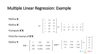
  • 30. Multiple Linear Regression: Example Student Test score IQ Study hours 1 100 110 40 2 90 120 30 3 80 100 20 4 70 90 0 5 60 80 10
  • 31. Multiple Linear Regression: Example •Define X. •Define X'. •Compute X'X. •Find the inverse of X'X. •Define Y.
  • 32. Multiple Linear Regression: Example b = (X'X)-1 X'Y ŷ = 20 + 0.5x1 +0.5x2
  • 33. Regression Types 1.Simple and Multiple Linear Regression 2.Logistic Regression 3.Polynomial Regression 4.Ridge Regression and Lasso Regression (upgrades to Linear Regression) 5.Decision Trees Regression 6.Support Vector Regression (SVR)
  • 34. Logistic Regression • Logistic Regression is used when the dependent variable(target) is categorical or binary. For example: • To predict whether an email is spam (1) or (0) • Whether the tumor is malignant (1) or not (0) • Logistic regression is widely used for classification problems • Logistic regression doesn’t require linear relationship between dependent and independent variables. • Logistic regression estimates the probability of an event belonging to a class, such as voted or didn’t vote.
  • 35. HR Analytics : IT firms recruit large number of people, but one of the problems they encounter is after accepting the job offer many candidates do not join. So, this results in cost over-runs because they have to repeat the entire process again. Now when you get an application, can you actually predict whether that applicant is likely to join the organization (Binary Outcome - Join / Not Join). Logistic Regression Example
  • 36. Why Logistic Regression In Linear regression, we draw a straight line(the best fit line) L1 such that the sum of distances of all the data points to the line is minimal.
  • 37. It uses sigmoid function is to map any predicted values of probabilities into another value between 0 and 1. Logistic Regression Equation Linear model: ŷ = b0+b1x Sigmoid function: σ(z) = 1/(1+e z − ) Logistic regression model: ŷ = σ(b0+b1x) = 1/(1+e-(b0+b1x) ) Also called logistic or logit function
  • 38. Logistic Regression Equation To make in the range from 0 to +infinity To make in the range from -infinity to +infinity Since we want to calculate value of p
  • 39. In logistic regression, as the output is a probability value between 0 or 1, mean squared error wouldn’t be the right choice. Instead, we use the log loss function which is derived from the maximum likelihood estimation method. Logistic Regression Evaluation
  • 41. Bias • Bias is simply defined as the inability of the model because of that there is some difference or error occurring between the model’s predicted value and the actual value. These differences between actual or expected values and the predicted values are known as error or bias error or error due to bias. • Let Y be the true value of a parameter, and let Y^ be an estimator of Y based on a sample of data. Then, the bias of the estimator Y^ is given by: • Bias(Y^)=E(Y^)–Y • where E(Y^) is the expected value of the estimator Y. It is the measurement of the model that how well it fits the data.
  • 42. Bias • Low Bias: Low bias value means fewer assumptions are taken to build the target function. In this case, the model will closely match the training dataset. • High Bias: High bias value means more assumptions are taken to build the target function. In this case, the model will not match the training dataset closely. • The high-bias model will not be able to capture the dataset trend. It is considered as the underfitting model which has a high error rate. It is due to a very simplified algorithm.
  • 43. Variance • The variance is the variability of the model that how much it is sensitive to another subset of the training dataset. i.e. how much it can adjust on the new subset of the training dataset. • Let Y be the actual values of the target variable, and Y^ be the predicted values of the target variable. • Then the variance of a model can be measured as the expected value of the square of the difference between predicted values and the expected value of the predicted values.
  • 44. • Variance=E[(Y^–E[Y^])2] • where E[Yˉ]E[Yˉ] is the expected value of the predicted values. Here expected value is averaged over all the training data. • Variance errors are either low or high-variance errors. • Low variance: Low variance means that the model is less sensitive to changes in the training data and can produce consistent estimates of the target function with different subsets of data from the same distribution. This is the case of underfitting when the model fails to generalize on both training and test data. • High variance: High variance means that the model is very sensitive to changes in the training data and can result in significant changes in the estimate of the target function when trained on different subsets of data from the same distribution. This is the case of overfitting when the model performs well on the training data but poorly on new, unseen test data. It fits the training data too closely that it fails on the new training dataset.
  • 45. Overfitting and Underfitting Underfitting is a situation when your model is too simple for your data or your hypothesis about data distribution is wrong and too simple. For example, your data is quadratic, and your model is linear. This situation is also called high bias. This means that your algorithm can do accurate predictions, but the initial assumption about the data is incorrect.
  • 46. Overfitting and Underfitting Overfitting is a situation when your model is too complex for your data. For example, your data is linear and your model is high- degree polynomial. This situation is also called high variance. In this situation, changing the input data only a little, the model output changes very much. •low bias, low variance — is a good result, just right. •low bias, high variance — overfitting — the algorithm outputs very different predictions for similar data. •high bias, low variance — underfitting — the algorithm outputs similar predictions for similar data, but predictions are wrong (algorithm “miss”). •high bias, high variance — very bad algorithm. You will most likely never see this.
  • 48. Regularization • Regularization is one of the ways to improve our model to work on unseen data by ignoring the less important features. • Regularization minimizes the validation loss and tries to improve the accuracy of the model. • It avoids overfitting by adding a penalty to the model with high variance.
  • 49. LASSO stands for Least Absolute Shrinkage and Selection Operator. Lasso regression performs L1 regularization, i.e. it adds a factor of sum of absolute value of coefficients in the optimization objective. This type of regularization (L1) can lead to zero coefficients i.e. some of the features are completely neglected for the evaluation of output. So, Lasso regression not only helps in reducing over- Lasso Regression
  • 50. In ridge regression, the cost function is altered by adding a penalty equivalent to square of the magnitude of the coefficients. The penalty term (lambda) regularizes the coefficients such that if the coefficients take large values the optimization function is penalized. Ridge regression shrinks the coefficients and it helps to reduce the model complexity and multi-collinearity It is also called “L2 regularization”. Ridge Regression
  • 51. Polynomial Regression • A regression equation is a polynomial regression equation if the power of independent variable is more than 1. The equation below represents a polynomial equation: • In this regression technique, the best fit line is not a straight line. It is rather a curve that fits into the data points.
  • 53. Regression vs Classification • Classification predictions can be evaluated using accuracy, whereas regression predictions cannot. • Regression predictions can be evaluated using root mean squared error, whereas classification predictions cannot. • A classification algorithm may predict a continuous value, but the continuous value is in the form of a probability for a class label. • A regression algorithm may predict a discrete value, but the discrete value in the form of an integer quantity.