SlideShare a Scribd company logo
Simple Linear Regression
Correlation
Correlation analyzes the LINEAR ASSOCIATION between two
variables. The CORRELATION COEFFICIENT (r) gives an
indication of the STRENGTH and DIRECTION of association
between the two variables.
Doesn’t differentiate between independent and dependent
variable
Eg: Height and Weight
Height and IQ
Regression
• Regression refers to the statistical technique of modeling the
relationship between variables.
• In simple linear regression, we model the relationship
between two variables.
• One of the variables, denoted by Y, is called the dependent
variable and the other, denoted by X, is called the
independent variable.
• The model we will use to depict the relationship between X
and Y will be a straight-line relationship (linear)
• A graphical sketch of the pairs (X, Y) is called a scatter plot.
Functional relationship between two or more variables and to
estimate (or predict) the unknown values of dependent variable
(Y) from the known values of independent variable (X).
This scatterplot locates pairs of observations of
advertising expenditures on the x-axis and sales
on the y-axis. We notice that:
.
Scatterplot of Advertising Expenditures (X) and Sales (Y)
50
40
30
20
10
0
140
120
100
80
60
40
20
0
A d vertising
S
ale
s
 The scatter of points tends to be distributed around a positively sloped straight line.
 The pairs of values of advertising expenditures and sales are not located exactly on a
straight line.
 The scatter plot reveals a more or less strong tendency rather than a precise linear
relationship.
 The line represents the nature of the relationship on average.
X
Y
X
Y
X 0
0
0
0
0
Y
X
Y
X
Y
X
Y
Examples of Other Scatterplots
6
Regression Analysis
In regression analysis we use the independent variable (X) to
estimate the dependent variable (Y).
• The relationship between the variables is linear.
• Both variables must be at least interval scale.
• The least squares criterion is used to determine the
equation.
Regression equation X on Y:
X = a + bY i
i
1
0
i ε
X
β
β
Y 


Random Error for this Xi
value
Y
X
Observed Value
of Y for Xi
Predicted Value
of Y for Xi
i
i
1
0
i ε
X
β
β
Y 


Xi
Slope = β1
Intercept = β0
εi
Simple Linear Regression Model
i
1
0
i x
b
b
y 

ˆ
The simple linear regression equation provides an estimate of the
population regression line
Simple Linear Regression Equation
Estimate of the
regression
intercept
Estimate of the
regression slope
Estimated (or
predicted) y
value for
observation i
Value of x for
observation i
The individual random error terms ei have a mean of zero
)
)
ˆ
( i
1
0
i
i
i
i x
b
(b
-
y
y
-
y
e 


Linear Regression Model
Assumptions
• The true relationship form is linear (Y is a linear function of X,
plus random error)
• The error terms, εi are independent of the x values
• The error terms are random variables with mean 0 and
constant variance, σ2
• The random error terms, εi, are not correlated with one
another
• No multicollinearity ( correlation between independent
variables)
• b0 (intercept) is the estimated average value
of y when the value of x is zero (if x = 0 is
in the range of observed x values)
• b1 (slope)is the estimated change in the
average value of y as a result of a one-unit
change in x
Interpretation of the
Slope and the Intercept
Find the regression equation on X on Y
Regression-SIMPLE LINEAR (1).psssssssssptx
Measures of Variation
• Total variation is made up of two parts:
SSE
SSR
SST 

Total Sum of
Squares
Regression Sum of
Squares
Error Sum of
Squares
 
 2
i )
y
(y
SST  
 2
i
i )
y
(y
SSE ˆ
 
 2
i )
y
y
(
SSR ˆ
where:
= Average value of the dependent variable
yi = Observed values of the dependent variable
i = Predicted value of y for the given xi value
ŷ
y
• SST = total sum of squares
– Measures the variation of the yi values around their
mean, y
• SSR = regression sum of squares
– Explained variation attributable to the linear
relationship between x and y
• SSE = error sum of squares
– Variation attributable to factors other than the linear
relationship between x and y
(continued)
Measures of Variation
• The coefficient of determination is the portion of
the total variation in the dependent variable that
is explained by variation in the independent
variable
• The coefficient of determination is also called R-
squared and is denoted as R2
Coefficient of Determination, R2
1
R
0 2


note:
squares
of
sum
total
squares
of
sum
regression
SST
SSR
R2


Chap 13-17
• Used to correct for the fact that adding non-relevant independent
variables will still reduce the error sum of squares
(where n = sample size, K = number of independent variables)
– Adjusted R2
provides a better comparison between
multiple regression models with different numbers of
independent variables
– Penalize excessive use of unimportant independent
variables
– Smaller than R2
(continued)
Adjusted Coefficient of
Determination, 2
R
1)
(n
/
SST
1)
K
(n
/
SSE
1
R2





Simple Linear Regression Example
• A real estate agent wishes to examine the relationship
between the selling price of a home and its size
(measured in square feet)
• A random sample of 10 houses is selected
– Dependent variable (Y) = house price in $1000s
– Independent variable (X) = square feet
Regression Analysis – Interpretation of Results
1. Explanatory Power: R-squared, Adjusted R-squared
gives you the ‘explanatory power’ of the set of
independent variables used in the model. It ranges
from zero to one, higher the better.
2. Goodness-of-fit: given by the significance of the F-
value. Only if the F-statistic is significant, your
regression model is good, else you need to revisit the
specification of your variables in the model.
3. Regression Coefficients: The standardized regression
coefficients give the extent and direction of influence of
a particular independent variable on the dependent
variable. The statistical significance of this coefficient
is given by the corresponding t-value.
Sample Data for House Price Model
House Price in $1000s
(Y)
Square Feet
(X)
245 1400
312 1600
279 1700
308 1875
199 1100
219 1550
405 2350
324 2450
319 1425
255 1700
Output
Regression Statistics
R Square 0.58082
Adjusted R Square 0.52842
Standard Error 41.33032
Observations 10
ANOVA
df SS MS F Significance F
Regression 1 18934.9348 18934.9348 11.0848 0.01039
Residual 8 13665.5652 1708.1957
Total 9 32600.5000
Coefficients Standard Error t Stat P-value Lower 95% Upper 95%
Intercept 98.24833 58.03348 1.69296 0.12892 -35.57720 232.07386
Square Feet 0.10977 0.03297 3.32938 0.01039 0.03374 0.18580
The regression equation is:
feet)
(square
0.10977
98.24833
price
house 

Prediction
• The regression equation can be used to
predict a value for y, given a particular x
• For a specified value, x , the predicted
value is
x
b
b
ŷ 1
0 

317.85
0)
0.1098(200
98.25
(sq.ft.)
0.1098
98.25
price
house





Predict the price for a house
with 2000 square feet:
The predicted price for a house with 2000
square feet is 317.85($1,000s) = $317,850
Predictions Using
Regression Analysis
Temperature Ice cream Sales (Y)
14.2 215
16.4 325
11.9 185
15.2 332
18.5 406
22.1 522
19.4 412
25.1 614
23.4 544
18.1 421
• Interpretation
92% of the variation in Ice-cream sales is
explained by the Temperature of the day
Significance of F < 0.05, X and Y are OK, else stop
P<0.05
Equation: Y = -159.474+30.92*X

More Related Content

Similar to Regression-SIMPLE LINEAR (1).psssssssssptx (20)

PPTX
Regression
Sauravurp
 
PPTX
Regression analysis
University of Jaffna
 
PPT
Statistics08_Cut_Regression.jdnkdjvbjddj
Nguyni223695
 
PPTX
REGRESSION METasdfghjklmjhgftrHODS1.pptx
cajativ595
 
PPTX
Stat 1163 -correlation and regression
Khulna University
 
PDF
Quantitative Methods - Level II - CFA Program
Mohamed Farouk, CFA, CFTe I
 
PPTX
Regression &amp; correlation coefficient
MuhamamdZiaSamad
 
PPTX
Introduction to Regression - The Importance.pptx
gilbertlucero2
 
PPTX
Regression
nandini patil
 
PPTX
CORRELATION AND REGRESSION.pptx
Rohit77460
 
PPTX
Regression refers to the statistical technique of modeling
AddisalemMenberu
 
PPT
Regression and Co-Relation
nuwan udugampala
 
PPT
simple linear regression statistics course
Saleh Abdelraouf Hussien
 
PPT
Research Methodology-Chapter 14
Javed Iqbal Kamyana
 
PPTX
Correlation and Regression Analysis.pptx
Unfold1
 
PPT
Corr-and-Regress.ppt
MoinPasha12
 
PPT
Corr-and-Regress.ppt
HarunorRashid74
 
PPT
Corr-and-Regress.ppt
krunal soni
 
PPT
Corr-and-Regress (1).ppt
MuhammadAftab89
 
Regression
Sauravurp
 
Regression analysis
University of Jaffna
 
Statistics08_Cut_Regression.jdnkdjvbjddj
Nguyni223695
 
REGRESSION METasdfghjklmjhgftrHODS1.pptx
cajativ595
 
Stat 1163 -correlation and regression
Khulna University
 
Quantitative Methods - Level II - CFA Program
Mohamed Farouk, CFA, CFTe I
 
Regression &amp; correlation coefficient
MuhamamdZiaSamad
 
Introduction to Regression - The Importance.pptx
gilbertlucero2
 
Regression
nandini patil
 
CORRELATION AND REGRESSION.pptx
Rohit77460
 
Regression refers to the statistical technique of modeling
AddisalemMenberu
 
Regression and Co-Relation
nuwan udugampala
 
simple linear regression statistics course
Saleh Abdelraouf Hussien
 
Research Methodology-Chapter 14
Javed Iqbal Kamyana
 
Correlation and Regression Analysis.pptx
Unfold1
 
Corr-and-Regress.ppt
MoinPasha12
 
Corr-and-Regress.ppt
HarunorRashid74
 
Corr-and-Regress.ppt
krunal soni
 
Corr-and-Regress (1).ppt
MuhammadAftab89
 

Recently uploaded (20)

PPTX
E-Way Bill under GST – Transport & Logistics.pptx
Keerthana Chinnathambi
 
PPTX
Struggling to Land a Social Media Marketing Job Here’s How to Navigate the In...
RahulSharma280537
 
PDF
🚀 Mohit Bansal_ Driving Urban Evolution Through GMI Infra (1).pdf
Mohit Bansal GMI
 
DOCX
Andrew C. Belton, MBA Resume - July 2025
Andrew C. Belton
 
PDF
NewBase 26 July 2025 Energy News issue - 1806 by Khaled Al Awadi_compressed.pdf
Khaled Al Awadi
 
PPTX
Appreciations - July 25.pptxdddddddddddss
anushavnayak
 
PDF
SMLE slides.pdf pediatric medical history
hananmahjoob18
 
PDF
Equinox Gold - Corporate Presentation.pdf
Equinox Gold Corp.
 
PDF
MBA-I-Year-Session-2024-20hzuxutiytidydy
cminati49
 
PPTX
FINAL _ DB x Forrester x Workday Webinar Buying Groups July 2025 (1).pptx
smarvin1
 
PDF
GenAI for Risk Management: Refresher for the Boards and Executives
Alexei Sidorenko, CRMP
 
DOCX
Navigating Environmental Excellence ISO 140012015 Implementation in Pretoria....
Norocke Consulting
 
DOCX
India's Emerging Global Leadership in Sustainable Energy Production The Rise ...
Insolation Energy
 
PDF
The New Zealand Business Sales Report 2025_compressed.pdf
charlie630518
 
PPTX
Brain Based Enterprises - Harmonising Man, Woman and Machine
Peter Cook
 
PPTX
The Rise of Artificial Intelligence pptx
divyamarya13
 
PDF
NewBase 24 July 2025 Energy News issue - 1805 by Khaled Al Awadi._compressed...
Khaled Al Awadi
 
PDF
Using Innovative Solar Manufacturing to Drive India's Renewable Energy Revolu...
Insolation Energy
 
PDF
Infrastructure and geopolitics.AM.ENG.docx.pdf
Andrea Mennillo
 
PPTX
E-commerce and its impact on business.
pandeyranjan5483
 
E-Way Bill under GST – Transport & Logistics.pptx
Keerthana Chinnathambi
 
Struggling to Land a Social Media Marketing Job Here’s How to Navigate the In...
RahulSharma280537
 
🚀 Mohit Bansal_ Driving Urban Evolution Through GMI Infra (1).pdf
Mohit Bansal GMI
 
Andrew C. Belton, MBA Resume - July 2025
Andrew C. Belton
 
NewBase 26 July 2025 Energy News issue - 1806 by Khaled Al Awadi_compressed.pdf
Khaled Al Awadi
 
Appreciations - July 25.pptxdddddddddddss
anushavnayak
 
SMLE slides.pdf pediatric medical history
hananmahjoob18
 
Equinox Gold - Corporate Presentation.pdf
Equinox Gold Corp.
 
MBA-I-Year-Session-2024-20hzuxutiytidydy
cminati49
 
FINAL _ DB x Forrester x Workday Webinar Buying Groups July 2025 (1).pptx
smarvin1
 
GenAI for Risk Management: Refresher for the Boards and Executives
Alexei Sidorenko, CRMP
 
Navigating Environmental Excellence ISO 140012015 Implementation in Pretoria....
Norocke Consulting
 
India's Emerging Global Leadership in Sustainable Energy Production The Rise ...
Insolation Energy
 
The New Zealand Business Sales Report 2025_compressed.pdf
charlie630518
 
Brain Based Enterprises - Harmonising Man, Woman and Machine
Peter Cook
 
The Rise of Artificial Intelligence pptx
divyamarya13
 
NewBase 24 July 2025 Energy News issue - 1805 by Khaled Al Awadi._compressed...
Khaled Al Awadi
 
Using Innovative Solar Manufacturing to Drive India's Renewable Energy Revolu...
Insolation Energy
 
Infrastructure and geopolitics.AM.ENG.docx.pdf
Andrea Mennillo
 
E-commerce and its impact on business.
pandeyranjan5483
 
Ad

Regression-SIMPLE LINEAR (1).psssssssssptx

  • 2. Correlation Correlation analyzes the LINEAR ASSOCIATION between two variables. The CORRELATION COEFFICIENT (r) gives an indication of the STRENGTH and DIRECTION of association between the two variables. Doesn’t differentiate between independent and dependent variable Eg: Height and Weight Height and IQ
  • 3. Regression • Regression refers to the statistical technique of modeling the relationship between variables. • In simple linear regression, we model the relationship between two variables. • One of the variables, denoted by Y, is called the dependent variable and the other, denoted by X, is called the independent variable. • The model we will use to depict the relationship between X and Y will be a straight-line relationship (linear) • A graphical sketch of the pairs (X, Y) is called a scatter plot. Functional relationship between two or more variables and to estimate (or predict) the unknown values of dependent variable (Y) from the known values of independent variable (X).
  • 4. This scatterplot locates pairs of observations of advertising expenditures on the x-axis and sales on the y-axis. We notice that: . Scatterplot of Advertising Expenditures (X) and Sales (Y) 50 40 30 20 10 0 140 120 100 80 60 40 20 0 A d vertising S ale s  The scatter of points tends to be distributed around a positively sloped straight line.  The pairs of values of advertising expenditures and sales are not located exactly on a straight line.  The scatter plot reveals a more or less strong tendency rather than a precise linear relationship.  The line represents the nature of the relationship on average.
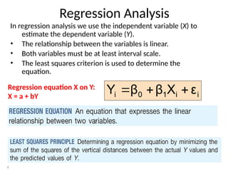
  • 6. 6 Regression Analysis In regression analysis we use the independent variable (X) to estimate the dependent variable (Y). • The relationship between the variables is linear. • Both variables must be at least interval scale. • The least squares criterion is used to determine the equation. Regression equation X on Y: X = a + bY i i 1 0 i ε X β β Y   
  • 7. Random Error for this Xi value Y X Observed Value of Y for Xi Predicted Value of Y for Xi i i 1 0 i ε X β β Y    Xi Slope = β1 Intercept = β0 εi Simple Linear Regression Model
  • 8. i 1 0 i x b b y   ˆ The simple linear regression equation provides an estimate of the population regression line Simple Linear Regression Equation Estimate of the regression intercept Estimate of the regression slope Estimated (or predicted) y value for observation i Value of x for observation i The individual random error terms ei have a mean of zero ) ) ˆ ( i 1 0 i i i i x b (b - y y - y e   
  • 9. Linear Regression Model Assumptions • The true relationship form is linear (Y is a linear function of X, plus random error) • The error terms, εi are independent of the x values • The error terms are random variables with mean 0 and constant variance, σ2 • The random error terms, εi, are not correlated with one another • No multicollinearity ( correlation between independent variables)
  • 10. • b0 (intercept) is the estimated average value of y when the value of x is zero (if x = 0 is in the range of observed x values) • b1 (slope)is the estimated change in the average value of y as a result of a one-unit change in x Interpretation of the Slope and the Intercept
  • 11. Find the regression equation on X on Y
  • 14. Measures of Variation • Total variation is made up of two parts: SSE SSR SST   Total Sum of Squares Regression Sum of Squares Error Sum of Squares    2 i ) y (y SST    2 i i ) y (y SSE ˆ    2 i ) y y ( SSR ˆ where: = Average value of the dependent variable yi = Observed values of the dependent variable i = Predicted value of y for the given xi value ŷ y
  • 15. • SST = total sum of squares – Measures the variation of the yi values around their mean, y • SSR = regression sum of squares – Explained variation attributable to the linear relationship between x and y • SSE = error sum of squares – Variation attributable to factors other than the linear relationship between x and y (continued) Measures of Variation
  • 16. • The coefficient of determination is the portion of the total variation in the dependent variable that is explained by variation in the independent variable • The coefficient of determination is also called R- squared and is denoted as R2 Coefficient of Determination, R2 1 R 0 2   note: squares of sum total squares of sum regression SST SSR R2  
  • 17. Chap 13-17 • Used to correct for the fact that adding non-relevant independent variables will still reduce the error sum of squares (where n = sample size, K = number of independent variables) – Adjusted R2 provides a better comparison between multiple regression models with different numbers of independent variables – Penalize excessive use of unimportant independent variables – Smaller than R2 (continued) Adjusted Coefficient of Determination, 2 R 1) (n / SST 1) K (n / SSE 1 R2     
  • 18. Simple Linear Regression Example • A real estate agent wishes to examine the relationship between the selling price of a home and its size (measured in square feet) • A random sample of 10 houses is selected – Dependent variable (Y) = house price in $1000s – Independent variable (X) = square feet
  • 19. Regression Analysis – Interpretation of Results 1. Explanatory Power: R-squared, Adjusted R-squared gives you the ‘explanatory power’ of the set of independent variables used in the model. It ranges from zero to one, higher the better. 2. Goodness-of-fit: given by the significance of the F- value. Only if the F-statistic is significant, your regression model is good, else you need to revisit the specification of your variables in the model. 3. Regression Coefficients: The standardized regression coefficients give the extent and direction of influence of a particular independent variable on the dependent variable. The statistical significance of this coefficient is given by the corresponding t-value.
  • 20. Sample Data for House Price Model House Price in $1000s (Y) Square Feet (X) 245 1400 312 1600 279 1700 308 1875 199 1100 219 1550 405 2350 324 2450 319 1425 255 1700
  • 21. Output Regression Statistics R Square 0.58082 Adjusted R Square 0.52842 Standard Error 41.33032 Observations 10 ANOVA df SS MS F Significance F Regression 1 18934.9348 18934.9348 11.0848 0.01039 Residual 8 13665.5652 1708.1957 Total 9 32600.5000 Coefficients Standard Error t Stat P-value Lower 95% Upper 95% Intercept 98.24833 58.03348 1.69296 0.12892 -35.57720 232.07386 Square Feet 0.10977 0.03297 3.32938 0.01039 0.03374 0.18580 The regression equation is: feet) (square 0.10977 98.24833 price house  
  • 22. Prediction • The regression equation can be used to predict a value for y, given a particular x • For a specified value, x , the predicted value is x b b ŷ 1 0  
  • 23. 317.85 0) 0.1098(200 98.25 (sq.ft.) 0.1098 98.25 price house      Predict the price for a house with 2000 square feet: The predicted price for a house with 2000 square feet is 317.85($1,000s) = $317,850 Predictions Using Regression Analysis
  • 24. Temperature Ice cream Sales (Y) 14.2 215 16.4 325 11.9 185 15.2 332 18.5 406 22.1 522 19.4 412 25.1 614 23.4 544 18.1 421
  • 25. • Interpretation 92% of the variation in Ice-cream sales is explained by the Temperature of the day Significance of F < 0.05, X and Y are OK, else stop P<0.05 Equation: Y = -159.474+30.92*X