SlideShare a Scribd company logo
3.1 Sampling Distributions
Contents:

                 Sampling Distributions
1.   Populations and Samples
2.   The Sampling Distribution of the mean ( known)
3.   The Sampling Distribution of the mean ( unknown)
4.   The Sampling Distribution of the Variance
Populations and Samples


                Finite
              Population
Population
               Infinite
              Population
Populations and Samples
Population: A set or collection of all the objects, actual
  or    conceptual      and    mainly      the  set     of
  numbers, measurements or observations which are
  under investigation.
Finite Population : All students in a College
Infinite Population : Total water in the sea or all the
  sand particle in sea shore.
Populations are often described by the distributions of
  their values, and it is common practice to refer to a
  population in terms of its distribution.
Finite Populations
• Finite populations are described by the actual
  distribution of its values and infinite populations are
  described by corresponding probability distribution or
  probability density.
• “Population f(x)” means a population is described
  by a frequency distribution, a probability distribution
  or a density f(x).
Infinite Population
If a population is infinite it is impossible to observe all
   its values, and even if it is finite it may be impractical
   or uneconomical to observe it in its entirety. Thus it is
   necessary to use a sample.
Sample: A part of population collected for investigation
   which needed to be representative of population and
   to be large enough to contain all information about
   population.
Random Sample (finite population):
• A set of observations X1, X2, …,Xn constitutes a
  random sample of size n from a finite
  population of size N, if its values are chosen so
  that each subset of n of the N elements of the
  population has the same probability of being
  selected.
Random Sample (infinite Population):
A set of observations X1, X2, …, Xn constitutes a random sample
     of size n from the infinite population ƒ(x) if:
      1. Each Xi is a random variable whose distribution is given
     by ƒ(x)
     2. These n random variables are independent.

We consider two types of random sample: those drawn with
   replacement and those drawn without replacement.
Sampling with replacement:
• In sampling with replacement, each object
  chosen is returned to the population before the
  next object is drawn. We define a random
  sample of size n drawn with replacement, as
  an ordered n-tuple of objects from the
  population, repetitions allowed.
The Space of random samples drawn with
              replacement:
 • If samples of size n are drawn with replacement from a
   population of size N, then there are Nn such samples. In any
   survey involving sample of size n, each of these should have
   same probability of being chosen. This is equivalent to making
   a collection of all Nn samples a probability space in which each
   sample has probability of being chosen 1/Nn.
 • Hence in above example There are 32 = 9 random samples of
   size 2 and each of the 9 random sample has probability 1/9 of
   being chosen.
Sampling without replacement:
In sampling without replacement, an object chosen is not returned
   to the population before the next object is drawn. We define
   random sample of size n, drawn without replacement as an
   unordered subset of n objects from the population.
The Space of random samples drawn
        without replacement:
• If sample of size n are drawn without
  replacement from a population of size N, then
            N    
  there are 
             n
               such samples. The collection of
                  
                  
                  

  all random samples drawn without
  replacement can be made into a probability
  space in which each sample has same chance
  of being selected.
Mean and Variance
If X1, X2, …, Xn constitute a random sample, then
                                        n

                                             X   i
                                       i 1
                        X 
                                              n
               is called the sample mean and
                                 n

                                      (X i  X )
                                                      2

                                i 1
                            
                        2
                    S
                                            n 1

                is called the sample variance.
Sampling distribution:
• The probability distribution of a random variable
  defined on a space of random samples is called a
  sampling distribution.
The Sampling Distribution of the Mean ( Known)

 Suppose that a random sample of n observations has been taken from
    some population and x has been computed, say, to estimate the mean
    of the population. If we take a second sample of size n from this
    population we get some different value for x . Similarly if we take
    several more samples and calculate x , probably no two of the x ' s     .
    would be alike. The difference among such x ' s are generally attributed
    to chance and this raises important question concerning their
    distribution, specially concerning the extent of their chance of
    fluctuations.
  Let  X and 
                  2
                  X
                      be mean and variance for sampling    distributi on of the
  mean X .
The Sampling Distribution of the Mean ( Known)

                           2
  Formula for μ X and σ X :
  Theorem 1: If a random sample of size n is taken from a population
  having the mean  and the variance 2, then X is a random variable
  whose distribution has the mean  .
                                                                             
                                                                               2

  For samples from infinite populations the variance of this distribution is     .
                                                                                           n
                                                                               N n
                                                                        2

  For samples from a finite population of size N the variance is n                    .
                                                                                N 1

                                      2
                                                  (for infinite   Population              )
                                      n
   That is  X   and             
                               2
                               X
                                        N n
                                         2
                                                   (for finite Population             )
                                      n N 1
                                     
The Sampling Distribution of the Mean ( Known)

 Proof of    for infinite population for the
                  X


   continuous
 case: From the definition we have
                      

     X      .....  x          f ( x1 , x 2 ,...., x n )dx 1 dx 2 .... dx n
                    
                            n
                                    xi
               .....            n
                                         f ( x1 , x 2 ,...., x n )dx 1 dx 2 .... dx n
                      i 1

                 n                 
            1
        
            n
                 .....  x            i
                                             f ( x1 , x 2 ,...., x n )dx 1 dx 2 .... dx n
                i 1            
The Sampling Distribution of the Mean ( Known


Where f(x1, x2, … , xn) is the joint density function of the random variables
which constitute the random sample. From the assumption of random sample
(for infinite population) each Xi is a random variable whose density function
is given by f(x) and these n random variables are independent, we can write
                   f(x1, x2, … , xn) = f(x1) f(x2) …… f(xn)
and we have
                    n               
               1
       X 
               n
                    .....  x          i
                                              f ( x1 ) f ( x 2 ).... f ( x n )dx 1 dx 2 .... dx n
                   i 1          

                    n                                                  
               1
           
               n
                            f ( x1 ) dx 1 ...  x i f ( x i ) dx i ....  f ( x n ) dx n
                   i 1                                             
The Sampling Distribution of the Mean ( Known)

Since each integral except the one with the integrand xi f(xi) equals 1 and the
one with the integrand xi f(xi) equals to , so we will have
                             n
                        1              1
                 X 
                        n
                                 
                                       n
                                           n   .
                            i 1

Note: for the discrete case the proof follows the same steps, with integral sign
replaced by  ' s.
For the proof of  X   2 / n we require the following result
                    2


Result: If X is a continuous random variable and Y = X - X , then Y = 0
   and hence  Y2   X .
                        2


Proof: Y = E(Y) = E(X - X) = E(X) - X = 0 and 
       Y2 = E[(Y - Y)2] = E [((X - X ) - 0)2] = E[(X - X)2] = X2.
The Sampling Distribution of the Mean ( Known)

• Regardless of the form of the population distribution, the
  distribution of     is approximately normal with mean  and
  variance 2/n whenever n is large.
• In practice, the normal distribution provides an excellent
                    X
  approximation to the sampling distribution of the mean
  for n as small as 25 or 30, with hardly any restrictions on the
  shape of the population.
• If the random samples come from a normal population, the
               X
  sampling distribution of the mean is normal regardless of
  the size of the sample.
The Sampling Distribution of the mean
               ( unknown)
• Application of the theory of previous section requires knowledge of the
  population standard deviation  .
• If n is large, this does not pose any problems even when  is unknown, as
  it is reasonable in that case to use for it the sample standard deviation s.
• However, when it comes to random variable whose values are given by
           very little is known about its exact sampling distribution for

   small values of n unless we make the assumption that the sample comes
   from a normal population.

                                 X  
                                           ,
                                 S /   n
The Sampling Distribution of the mean
            ( unknown)
 Theorem : If     is the mean of a random sample of size n taken from a
   normal population having the mean  and the variance 2, and
             X


                      (Xi  X )
                n                 2

                                    , then
       2
   S
               i 1     n 1
                                       X 
                               t
                       S/ n
is a random variable having the t distribution with the parameter  = n – 1.
This theorem is more general than Theorem 6.2 in the sense that it does not
require knowledge of  ; on the other hand, it is less general than Theorem 6.2
in the sense that it requires the assumption of a normal population.
The Sampling Distribution of the mean
           ( unknown)
• The t distribution was introduced by William S.Gosset in
  1908, who published his scientific paper under the pen name
  “Student,” since his company did not permit publication by
  employees. That’s why t distribution is also known as the
  Student-t distribution, or Student’s           t distribution.
• The shape of t distribution is similar to that of a normal
  distribution i.e. both are bell-shaped and symmetric about the
  mean.
• Like the standard normal distribution, the t distribution has the
  mean 0, but its variance depends on the parameter , called the
  number of degrees of freedom.
The Sampling Distribution of the mean
           ( unknown)


                                      t ( =10)
                  Normal


                           t ( =1)


 Figure: t distribution and standard normal distributions
The Sampling Distribution of the mean
              ( unknown)
• When   , the t distribution approaches the standard
  normal distribution i.e. when   , t  z.
• The standard normal distribution provides a good
  approximation to the t distribution for samples of size 30 or
  more.

More Related Content

What's hot (20)

PPTX
Point Estimation
DataminingTools Inc
 
PPTX
Statistical inference: Estimation
Parag Shah
 
PPT
The sampling distribution
Harve Abella
 
PPTX
Discrete distributions: Binomial, Poisson & Hypergeometric distributions
ScholarsPoint1
 
PPTX
Binomial probability distributions
Long Beach City College
 
PPTX
T distribution
Stephan Jade Navarro
 
PPTX
Hypothesis Testing
Kalyan Acharjya
 
PPT
PROBABILITY AND PROBABILITY DISTRIBUTIONS.ppt
JimbertTingcang2
 
DOCX
Probability distribution
Rohit kumar
 
PPT
Hypothesis
Nilanjan Bhaumik
 
PPT
Ppt for 1.1 introduction to statistical inference
vasu Chemistry
 
PDF
Probability Distributions
CIToolkit
 
PPT
Confidence Intervals
mandalina landy
 
PPTX
Central limit theorem
Nadeem Uddin
 
PPTX
Goodness of fit (ppt)
Sharlaine Ruth
 
PPTX
Central limit theorem
Vijeesh Soman
 
DOCX
Estimation in statistics
Rabea Jamal
 
PDF
Sampling and sampling distribution tttt
pardeepkaur60
 
PPTX
binomial distribution
Mmedsc Hahm
 
PPTX
Binomial distribution
numanmunir01
 
Point Estimation
DataminingTools Inc
 
Statistical inference: Estimation
Parag Shah
 
The sampling distribution
Harve Abella
 
Discrete distributions: Binomial, Poisson & Hypergeometric distributions
ScholarsPoint1
 
Binomial probability distributions
Long Beach City College
 
T distribution
Stephan Jade Navarro
 
Hypothesis Testing
Kalyan Acharjya
 
PROBABILITY AND PROBABILITY DISTRIBUTIONS.ppt
JimbertTingcang2
 
Probability distribution
Rohit kumar
 
Hypothesis
Nilanjan Bhaumik
 
Ppt for 1.1 introduction to statistical inference
vasu Chemistry
 
Probability Distributions
CIToolkit
 
Confidence Intervals
mandalina landy
 
Central limit theorem
Nadeem Uddin
 
Goodness of fit (ppt)
Sharlaine Ruth
 
Central limit theorem
Vijeesh Soman
 
Estimation in statistics
Rabea Jamal
 
Sampling and sampling distribution tttt
pardeepkaur60
 
binomial distribution
Mmedsc Hahm
 
Binomial distribution
numanmunir01
 

Similar to Sampling Distributions (20)

PPTX
Sampling Distributions
mathscontent
 
PPTX
Hypergeometric Distribution
DataminingTools Inc
 
PPTX
Hypergeometric Distribution
mathscontent
 
PDF
Basics of probability in statistical simulation and stochastic programming
SSA KPI
 
PPTX
1853_Random Variable & Distribution.pptx
quantjsam
 
DOCX
UNIT -3 SAMPLING DISTRIBUTION .docx
surendhardevireddy04
 
PPT
sampling distribution
Mmedsc Hahm
 
PDF
lecture4.pdf
TarikuArega1
 
PPT
Doe02 statistics
Arif Rahman
 
PDF
Ssp notes
balu902
 
PDF
Intro probability 4
Phong Vo
 
PDF
Statistics (1): estimation, Chapter 1: Models
Christian Robert
 
PDF
Welcome to International Journal of Engineering Research and Development (IJERD)
IJERD Editor
 
PPTX
7.-Mean-And-Variance_______________.pptx
JurenEnopia
 
PPT
Probability and random process Chapter two-Random_Variables.ppt
getahunshanko2024
 
PDF
Robustness under Independent Contamination Model
rusmike
 
PDF
ttest_intro.pdf
UMAIRASHFAQ20
 
PPTX
ISM_Session_5 _ 23rd and 24th December.pptx
ssuser1eba67
 
PPT
LSCM 2072_chapter 1.ppt social marketing management
DagimNegash1
 
Sampling Distributions
mathscontent
 
Hypergeometric Distribution
DataminingTools Inc
 
Hypergeometric Distribution
mathscontent
 
Basics of probability in statistical simulation and stochastic programming
SSA KPI
 
1853_Random Variable & Distribution.pptx
quantjsam
 
UNIT -3 SAMPLING DISTRIBUTION .docx
surendhardevireddy04
 
sampling distribution
Mmedsc Hahm
 
lecture4.pdf
TarikuArega1
 
Doe02 statistics
Arif Rahman
 
Ssp notes
balu902
 
Intro probability 4
Phong Vo
 
Statistics (1): estimation, Chapter 1: Models
Christian Robert
 
Welcome to International Journal of Engineering Research and Development (IJERD)
IJERD Editor
 
7.-Mean-And-Variance_______________.pptx
JurenEnopia
 
Probability and random process Chapter two-Random_Variables.ppt
getahunshanko2024
 
Robustness under Independent Contamination Model
rusmike
 
ttest_intro.pdf
UMAIRASHFAQ20
 
ISM_Session_5 _ 23rd and 24th December.pptx
ssuser1eba67
 
LSCM 2072_chapter 1.ppt social marketing management
DagimNegash1
 
Ad

More from DataminingTools Inc (20)

PPTX
Terminology Machine Learning
DataminingTools Inc
 
PPTX
Techniques Machine Learning
DataminingTools Inc
 
PPTX
Machine learning Introduction
DataminingTools Inc
 
PPTX
Areas of machine leanring
DataminingTools Inc
 
PPTX
AI: Planning and AI
DataminingTools Inc
 
PPTX
AI: Logic in AI 2
DataminingTools Inc
 
PPTX
AI: Logic in AI
DataminingTools Inc
 
PPTX
AI: Learning in AI 2
DataminingTools Inc
 
PPTX
AI: Learning in AI
DataminingTools Inc
 
PPTX
AI: Introduction to artificial intelligence
DataminingTools Inc
 
PPTX
AI: Belief Networks
DataminingTools Inc
 
PPTX
AI: AI & Searching
DataminingTools Inc
 
PPTX
AI: AI & Problem Solving
DataminingTools Inc
 
PPTX
Data Mining: Text and web mining
DataminingTools Inc
 
PPTX
Data Mining: Outlier analysis
DataminingTools Inc
 
PPTX
Data Mining: Mining stream time series and sequence data
DataminingTools Inc
 
PPTX
Data Mining: Mining ,associations, and correlations
DataminingTools Inc
 
PPTX
Data Mining: Graph mining and social network analysis
DataminingTools Inc
 
PPTX
Data warehouse and olap technology
DataminingTools Inc
 
PPTX
Data Mining: Data processing
DataminingTools Inc
 
Terminology Machine Learning
DataminingTools Inc
 
Techniques Machine Learning
DataminingTools Inc
 
Machine learning Introduction
DataminingTools Inc
 
Areas of machine leanring
DataminingTools Inc
 
AI: Planning and AI
DataminingTools Inc
 
AI: Logic in AI 2
DataminingTools Inc
 
AI: Logic in AI
DataminingTools Inc
 
AI: Learning in AI 2
DataminingTools Inc
 
AI: Learning in AI
DataminingTools Inc
 
AI: Introduction to artificial intelligence
DataminingTools Inc
 
AI: Belief Networks
DataminingTools Inc
 
AI: AI & Searching
DataminingTools Inc
 
AI: AI & Problem Solving
DataminingTools Inc
 
Data Mining: Text and web mining
DataminingTools Inc
 
Data Mining: Outlier analysis
DataminingTools Inc
 
Data Mining: Mining stream time series and sequence data
DataminingTools Inc
 
Data Mining: Mining ,associations, and correlations
DataminingTools Inc
 
Data Mining: Graph mining and social network analysis
DataminingTools Inc
 
Data warehouse and olap technology
DataminingTools Inc
 
Data Mining: Data processing
DataminingTools Inc
 
Ad

Recently uploaded (20)

PPTX
FAMILY HEALTH NURSING CARE - UNIT 5 - CHN 1 - GNM 1ST YEAR.pptx
Priyanshu Anand
 
PDF
EXCRETION-STRUCTURE OF NEPHRON,URINE FORMATION
raviralanaresh2
 
PPTX
IDEAS AND EARLY STATES Social science pptx
NIRANJANASSURESH
 
PPTX
Gupta Art & Architecture Temple and Sculptures.pptx
Virag Sontakke
 
PPTX
Cleaning Validation Ppt Pharmaceutical validation
Ms. Ashatai Patil
 
PPTX
Electrophysiology_of_Heart. Electrophysiology studies in Cardiovascular syste...
Rajshri Ghogare
 
DOCX
pgdei-UNIT -V Neurological Disorders & developmental disabilities
JELLA VISHNU DURGA PRASAD
 
PPTX
Basics and rules of probability with real-life uses
ravatkaran694
 
PPTX
The Future of Artificial Intelligence Opportunities and Risks Ahead
vaghelajayendra784
 
PDF
Tips for Writing the Research Title with Examples
Thelma Villaflores
 
PDF
BÀI TẬP TEST BỔ TRỢ THEO TỪNG CHỦ ĐỀ CỦA TỪNG UNIT KÈM BÀI TẬP NGHE - TIẾNG A...
Nguyen Thanh Tu Collection
 
PPT
DRUGS USED IN THERAPY OF SHOCK, Shock Therapy, Treatment or management of shock
Rajshri Ghogare
 
PDF
Virat Kohli- the Pride of Indian cricket
kushpar147
 
PPTX
Virus sequence retrieval from NCBI database
yamunaK13
 
PPTX
Top 10 AI Tools, Like ChatGPT. You Must Learn In 2025
Digilearnings
 
PPTX
Various Psychological tests: challenges and contemporary trends in psychologi...
santoshmohalik1
 
PPTX
Translation_ Definition, Scope & Historical Development.pptx
DhatriParmar
 
PDF
Exploring-the-Investigative-World-of-Science.pdf/8th class curiosity/1st chap...
Sandeep Swamy
 
PPTX
Unlock the Power of Cursor AI: MuleSoft Integrations
Veera Pallapu
 
PPTX
Introduction to pediatric nursing in 5th Sem..pptx
AneetaSharma15
 
FAMILY HEALTH NURSING CARE - UNIT 5 - CHN 1 - GNM 1ST YEAR.pptx
Priyanshu Anand
 
EXCRETION-STRUCTURE OF NEPHRON,URINE FORMATION
raviralanaresh2
 
IDEAS AND EARLY STATES Social science pptx
NIRANJANASSURESH
 
Gupta Art & Architecture Temple and Sculptures.pptx
Virag Sontakke
 
Cleaning Validation Ppt Pharmaceutical validation
Ms. Ashatai Patil
 
Electrophysiology_of_Heart. Electrophysiology studies in Cardiovascular syste...
Rajshri Ghogare
 
pgdei-UNIT -V Neurological Disorders & developmental disabilities
JELLA VISHNU DURGA PRASAD
 
Basics and rules of probability with real-life uses
ravatkaran694
 
The Future of Artificial Intelligence Opportunities and Risks Ahead
vaghelajayendra784
 
Tips for Writing the Research Title with Examples
Thelma Villaflores
 
BÀI TẬP TEST BỔ TRỢ THEO TỪNG CHỦ ĐỀ CỦA TỪNG UNIT KÈM BÀI TẬP NGHE - TIẾNG A...
Nguyen Thanh Tu Collection
 
DRUGS USED IN THERAPY OF SHOCK, Shock Therapy, Treatment or management of shock
Rajshri Ghogare
 
Virat Kohli- the Pride of Indian cricket
kushpar147
 
Virus sequence retrieval from NCBI database
yamunaK13
 
Top 10 AI Tools, Like ChatGPT. You Must Learn In 2025
Digilearnings
 
Various Psychological tests: challenges and contemporary trends in psychologi...
santoshmohalik1
 
Translation_ Definition, Scope & Historical Development.pptx
DhatriParmar
 
Exploring-the-Investigative-World-of-Science.pdf/8th class curiosity/1st chap...
Sandeep Swamy
 
Unlock the Power of Cursor AI: MuleSoft Integrations
Veera Pallapu
 
Introduction to pediatric nursing in 5th Sem..pptx
AneetaSharma15
 

Sampling Distributions

  • 2. Contents: Sampling Distributions 1. Populations and Samples 2. The Sampling Distribution of the mean ( known) 3. The Sampling Distribution of the mean ( unknown) 4. The Sampling Distribution of the Variance
  • 3. Populations and Samples Finite Population Population Infinite Population
  • 4. Populations and Samples Population: A set or collection of all the objects, actual or conceptual and mainly the set of numbers, measurements or observations which are under investigation. Finite Population : All students in a College Infinite Population : Total water in the sea or all the sand particle in sea shore. Populations are often described by the distributions of their values, and it is common practice to refer to a population in terms of its distribution.
  • 5. Finite Populations • Finite populations are described by the actual distribution of its values and infinite populations are described by corresponding probability distribution or probability density. • “Population f(x)” means a population is described by a frequency distribution, a probability distribution or a density f(x).
  • 6. Infinite Population If a population is infinite it is impossible to observe all its values, and even if it is finite it may be impractical or uneconomical to observe it in its entirety. Thus it is necessary to use a sample. Sample: A part of population collected for investigation which needed to be representative of population and to be large enough to contain all information about population.
  • 7. Random Sample (finite population): • A set of observations X1, X2, …,Xn constitutes a random sample of size n from a finite population of size N, if its values are chosen so that each subset of n of the N elements of the population has the same probability of being selected.
  • 8. Random Sample (infinite Population): A set of observations X1, X2, …, Xn constitutes a random sample of size n from the infinite population ƒ(x) if: 1. Each Xi is a random variable whose distribution is given by ƒ(x) 2. These n random variables are independent. We consider two types of random sample: those drawn with replacement and those drawn without replacement.
  • 9. Sampling with replacement: • In sampling with replacement, each object chosen is returned to the population before the next object is drawn. We define a random sample of size n drawn with replacement, as an ordered n-tuple of objects from the population, repetitions allowed.
  • 10. The Space of random samples drawn with replacement: • If samples of size n are drawn with replacement from a population of size N, then there are Nn such samples. In any survey involving sample of size n, each of these should have same probability of being chosen. This is equivalent to making a collection of all Nn samples a probability space in which each sample has probability of being chosen 1/Nn. • Hence in above example There are 32 = 9 random samples of size 2 and each of the 9 random sample has probability 1/9 of being chosen.
  • 11. Sampling without replacement: In sampling without replacement, an object chosen is not returned to the population before the next object is drawn. We define random sample of size n, drawn without replacement as an unordered subset of n objects from the population.
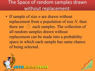
  • 12. The Space of random samples drawn without replacement: • If sample of size n are drawn without replacement from a population of size N, then N  there are   n  such samples. The collection of    all random samples drawn without replacement can be made into a probability space in which each sample has same chance of being selected.
  • 13. Mean and Variance If X1, X2, …, Xn constitute a random sample, then n  X i i 1 X  n is called the sample mean and n  (X i  X ) 2 i 1  2 S n 1 is called the sample variance.
  • 14. Sampling distribution: • The probability distribution of a random variable defined on a space of random samples is called a sampling distribution.
  • 15. The Sampling Distribution of the Mean ( Known) Suppose that a random sample of n observations has been taken from some population and x has been computed, say, to estimate the mean of the population. If we take a second sample of size n from this population we get some different value for x . Similarly if we take several more samples and calculate x , probably no two of the x ' s . would be alike. The difference among such x ' s are generally attributed to chance and this raises important question concerning their distribution, specially concerning the extent of their chance of fluctuations. Let  X and  2 X be mean and variance for sampling distributi on of the mean X .
  • 16. The Sampling Distribution of the Mean ( Known) 2 Formula for μ X and σ X : Theorem 1: If a random sample of size n is taken from a population having the mean  and the variance 2, then X is a random variable whose distribution has the mean  .  2 For samples from infinite populations the variance of this distribution is . n  N n 2 For samples from a finite population of size N the variance is n  . N 1  2  (for infinite Population )  n That is  X   and    2 X  N n 2  (for finite Population )  n N 1 
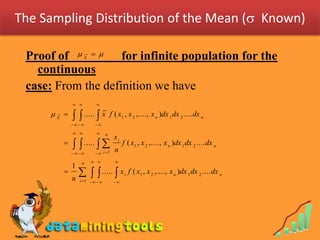
  • 17. The Sampling Distribution of the Mean ( Known) Proof of    for infinite population for the X continuous case: From the definition we have    X    .....  x f ( x1 , x 2 ,...., x n )dx 1 dx 2 .... dx n      n xi    .....   n f ( x1 , x 2 ,...., x n )dx 1 dx 2 .... dx n    i 1 n    1  n    .....  x i f ( x1 , x 2 ,...., x n )dx 1 dx 2 .... dx n i 1     
  • 18. The Sampling Distribution of the Mean ( Known Where f(x1, x2, … , xn) is the joint density function of the random variables which constitute the random sample. From the assumption of random sample (for infinite population) each Xi is a random variable whose density function is given by f(x) and these n random variables are independent, we can write f(x1, x2, … , xn) = f(x1) f(x2) …… f(xn) and we have n    1 X  n    .....  x i f ( x1 ) f ( x 2 ).... f ( x n )dx 1 dx 2 .... dx n i 1      n    1  n   f ( x1 ) dx 1 ...  x i f ( x i ) dx i ....  f ( x n ) dx n i 1    
  • 19. The Sampling Distribution of the Mean ( Known) Since each integral except the one with the integrand xi f(xi) equals 1 and the one with the integrand xi f(xi) equals to , so we will have n 1 1 X  n   n n   . i 1 Note: for the discrete case the proof follows the same steps, with integral sign replaced by  ' s. For the proof of  X   2 / n we require the following result 2 Result: If X is a continuous random variable and Y = X - X , then Y = 0 and hence  Y2   X . 2 Proof: Y = E(Y) = E(X - X) = E(X) - X = 0 and  Y2 = E[(Y - Y)2] = E [((X - X ) - 0)2] = E[(X - X)2] = X2.
  • 20. The Sampling Distribution of the Mean ( Known) • Regardless of the form of the population distribution, the distribution of is approximately normal with mean  and variance 2/n whenever n is large. • In practice, the normal distribution provides an excellent X approximation to the sampling distribution of the mean for n as small as 25 or 30, with hardly any restrictions on the shape of the population. • If the random samples come from a normal population, the X sampling distribution of the mean is normal regardless of the size of the sample.
  • 21. The Sampling Distribution of the mean ( unknown) • Application of the theory of previous section requires knowledge of the population standard deviation  . • If n is large, this does not pose any problems even when  is unknown, as it is reasonable in that case to use for it the sample standard deviation s. • However, when it comes to random variable whose values are given by very little is known about its exact sampling distribution for small values of n unless we make the assumption that the sample comes from a normal population. X   , S / n
  • 22. The Sampling Distribution of the mean ( unknown) Theorem : If is the mean of a random sample of size n taken from a normal population having the mean  and the variance 2, and X (Xi  X ) n 2   , then 2 S i 1 n 1 X  t S/ n is a random variable having the t distribution with the parameter  = n – 1. This theorem is more general than Theorem 6.2 in the sense that it does not require knowledge of  ; on the other hand, it is less general than Theorem 6.2 in the sense that it requires the assumption of a normal population.
  • 23. The Sampling Distribution of the mean ( unknown) • The t distribution was introduced by William S.Gosset in 1908, who published his scientific paper under the pen name “Student,” since his company did not permit publication by employees. That’s why t distribution is also known as the Student-t distribution, or Student’s t distribution. • The shape of t distribution is similar to that of a normal distribution i.e. both are bell-shaped and symmetric about the mean. • Like the standard normal distribution, the t distribution has the mean 0, but its variance depends on the parameter , called the number of degrees of freedom.
  • 24. The Sampling Distribution of the mean ( unknown) t ( =10) Normal t ( =1) Figure: t distribution and standard normal distributions
  • 25. The Sampling Distribution of the mean ( unknown) • When   , the t distribution approaches the standard normal distribution i.e. when   , t  z. • The standard normal distribution provides a good approximation to the t distribution for samples of size 30 or more.