Searching and Sorting algorithms and working

Sorting & Searching
 Searching
 Linear/Sequential Search
 Binary Search
 Sorting
 Sélection Sort
 Bubble sort
 Quick Sort
 Merge Sort

Linear/Sequential Search
 In computer science, linear search or sequential search is a method for
finding a particular value in a list that consists of checking every one of its
elements, one at a time and in sequence, until the desired one is found.
 Linear search is the simplest search algorithm.
 It is a special case of brute-force search.
 Its worst case cost is proportional to the number of elements in the list.

Sequential Search – Algorithm & Example
# Input: Array A, integer key
# Output: first index of key
in A
# or -1 if not found
Algorithm: Linear_Search
for i = 0 to last index of A:
if A[i] equals key:
return i
return -1
Search for 1 in given array 2 9 3 1 8
Comparing value of ith
index with element to be search one by
one until we get searched element or end of the array
Step 1: i=0
2 9 3 1 8
i
Step 1: i=1
2 9 3 1 8
i
Step 1: i=2
2 9 3 1 8
i
Step 1: i=3
2 9 3 1 8
i
1
Element found at ith
index, i=3

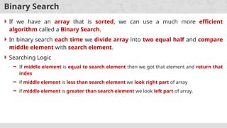
Binary Search
 If we have an array that is sorted, we can use a much more efficient
algorithm called a Binary Search.
 In binary search each time we divide array into two equal half and compare
middle element with search element.
 Searching Logic
 If middle element is equal to search element then we got that element and return that
index
 if middle element is less than search element we look right part of array
 if middle element is greater than search element we look left part of array.

Binary Search - Algorithm
Search for 6 in given array
-1 5 6 18 19 25 46 78 102 114
Key=6, No of Elements = 10, so left = 0, right=9
0 1 2 3 4 5 6 7 8 9
Index
middle index = (left + right) /2 = (0+9)/2 = 4
middle element value = a[4] = 19
Key=6 is less than middle element = 19, so right = middle – 1 = 4 – 1 = 3, left = 0
-1 5 6 18 19 25 46 78 102 114
0 1 2 3 4 5 6 7 8 9
Index
left right
left right
Step 1:

Key=6 is greater than middle element = 5, so left = middle + 1 =1 + 1 = 2, right = 3
-1 5 6 18 19 25 46 78 102 114
0 1 2 3 4 5 6 7 8 9
Index
left right
Step 2:
Key=6 is equals to middle element = 6, so element found
-1 5 6 18 19 25 46 78 102 114
0 1 2 3 4 5 6 7 8 9
Index
Element Found
Step 3:
6

# Input: Sorted Array A, integer key
# Output: first index of key in A,
# or -1 if not found
Algorithm: Binary_Search (A, left, right)
left = 0, right = n-1
while left < right
middle = index halfway between left, right
if A[middle] matches key
return middle
else if key less than A[middle]
right = middle -1
else
left = middle + 1
return -1

Selection Sort
 Selection sort is a simple sorting algorithm.
 The list is divided into two parts,
 The sorted part at the left end and
 The unsorted part at the right end.
 Initially, the sorted part is empty and the unsorted part is the entire list.
 The smallest element is selected from the unsorted array and swapped with
the leftmost element, and that element becomes a part of the sorted array.
 This process continues moving unsorted array boundary by one element to the
right.
 This algorithm is not suitable for large data sets as its average and worst case
complexities are of Ο(n2
), where n is the number of items.

Selection Sort
5 1 12 -5 16 2 12 14
Unsorted Array
Step 1 :
5 1 12 -5 16 2 12 14
Unsorted Array
0 1 2 3 4 5 6 7
Step 2 :
Min index = 0, value = 5
5 1 12 -5 16 2 12 14
0 1 2 3 4 5 6 7
Find min value from
Unsorted array
Index = 3, value = -5
Unsorted Array (elements 0 to
7)
Swap
-5 5

Selection Sort
Step 3 :
-5 1 12 5 16 2 12 14
0 1 2 3 4 5 6 7
Unsorted Array (elements 1
to 7)
Find min value from
Unsorted array
Index = 1, value = 1
No Swapping as min value is already at right place
1
Step 4 :
-5 1 12 5 16 2 12 14
0 1 2 3 4 5 6 7
Unsorted Array
(elements 2 to 7)
Find min value from
Unsorted array
Swap
2 12

Selection Sort
Step 5 :
-5 1 2 5 16 12 12 14
0 1 2 3 4 5 6 7
Find min value from
Unsorted array
Step 6 :
-5 1 2 5 16 12 12 14
0 1 2 3 4 5 6 7
Find min value from
Unsorted array
Swap
Unsorted Array
(elements 3 to 7)
No Swapping as min value is already at right place
5
Unsorted Array
(elements 5 to 7)
12 16

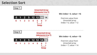
Selection Sort
Step 7 :
-5 1 2 5 12 16 12 14
0 1 2 3 4 5 6 7
Find min value from
Unsorted array
Swap
12 16
Unsorted Array
(elements 5 to 7)
-5 1 2 5 12 12 16 14
0 1 2 3 4 5 6 7
Find min value from
Unsorted array
Swap
14 16
Unsorted Array
(elements 6 to 7)
Step 8 :

SELECTION_SORT(K,N)
 Given a vector K of N elements
 This procedure rearrange the vector in ascending order using Selection Sort
 The variable PASS denotes the pass index and position of the first element in
the vector
 The variable MIN_INDEX denotes the position of the smallest element
encountered
 The variable I is used to index elements

SELECTION_SORT(K,N)
1. [Loop on the Pass index]
Repeat thru step 4 for PASS = 0,1,…….., N-2
2. [Initialize minimum index]
MIN_INDEX  PASS
3. [Make a pass and obtain element with smallest value]
Repeat for I = PASS + 1, PASS + 2, …………….., N-1
If K[I] < K[MIN_INDEX]
Then MIN_INDEX  I
4. [Exchange elements]
IF MIN_INDEX <> PASS
Then K[PASS]  K[MIN_INDEX]
5. [Finished]
Return

Bubble Sort
 Unlike selection sort, instead of finding the smallest record and performing
the interchange, two records are interchanged immediately upon discovering
that they are out of order
 During the first pass R1 and R2 are compared and interchanged in case of
our of order, this process is repeated for records R2 and R3, and so on.
 This method will cause records with small key to move “bubble up”,
 After the first pass, the record with largest key will be in the nth
position.
 On each successive pass, the records with the next largest key will be placed in
position n-1, n-2 ….., 2 respectively
 This approached required at most n–1 passes, The complexity of bubble sort is
O(n2
)

Bubble Sort
45 34 56 23 12
Unsorted Array
Pass 1 :
45
34
56
23
12
34
45
56
23
12
34
45
56
23
12
34
45
23
56
12
34
45
swap
swap
23
56
swap
12
56
Pass 2 :
34
45
23
12
56
34
45
23
12
56
34
23
45
12
56
34
23
12
45
56
swap
23
45
swap
12
45
Pass 3 :
23
34
12
45
56
23
12
34
45
56
swap
23
34
swap
12
34
Pass 4 :
swap
12
23

BUBBLE_SORT(K,N)
 Given a vector K of N elements
 This procedure rearrange the vector in ascending order using Bubble Sort
 The variable PASS & LAST denotes the pass index and position of the first
element in the vector
 The variable EXCHS is used to count number of exchanges made on any pass
 The variable I is used to index elements

Procedure: BUBBLE_SORT (K, N)
1. [Initialize]
LAST  N-1
2. [Loop on pass index]
Repeat thru step 5 for PASS = 0, 1, 2, …. , N-2
3. [Initialize exchange counter for this pass]
EXCHS  0
4. [Perform pairwise comparisons on unsorted elements]
Repeat for I = 0, 1, ……….., LAST – 1
IF K[I] > K [I+1]
Then K[I]  K[I+1]
EXCHS  EXCHS + 1
5. [Any exchange made in this pass?]
IF EXCHS = 0
Then Return (Vector is sorted, early return)
ELSE LAST  LAST - 1
6. [Finished]
Return

Quick Sort
 Quick sort is a highly efficient sorting algorithm and is based on partitioning
of array of data into smaller arrays.
 Quick Sort is divide and conquer algorithm.
 At each step of the method, the goal is to place a particular record in its final
position within the table,
 In doing so all the records which precedes this record will have smaller keys,
while all records that follows it have larger keys.
 This particular record is termed pivot element.
 The same process can then be applied to each of these sub-tables and
repeated until all records are placed in their positions

Quick Sort
 There are many different versions of Quick Sort that pick pivot in different
ways.
 Always pick first element as pivot. (in our case we have consider this version).
 Always pick last element as pivot
 Pick a random element as pivot.
 Pick median as pivot.
 Quick sort partitions an array and then calls itself recursively twice to sort the
two resulting sub arrays.
 This algorithm is quite efficient for large-sized data sets
 Its average and worst case complexity are of Ο(n2
), where n is the number of
items.

Quick Sort
42 23 74 11 65 58 94 36
0 1 2 3 4 5 6 7
99 87
8 9
LB UB
Pivot
Element
Sort Following Array using Quick Sort Algorithm
We are considering first element as pivot element, so Lower bound is First
Index and Upper bound is Last Index
We need to find our proper position of Pivot element in sorted array and
perform same operations recursively for two sub array

Quick Sort
42 23 74 11 65 58 94 36
0 1 2 3 4 5 6 7
99 87
8 9
FLAG  true
IF LB < UB
Then
I  LB
J  UB + 1
KEY  K[LB]
Repeat While FLAG = true
I  I+1
Repeat While K[I] < KEY
I  I + 1
J  J – 1
Repeat While K[J] > KEY
J  J – 1
IF I<J
Then K[I] --- K[J]
Else FLAG  FALSE
K[LB] --- K[J]
LB = 0, UB = 9
I= 0
J= 10
KEY = 42
I J
FLAG=
true
42 23 74 11 65 58 94 36 99 87
I J
36 74
Swap
42 23 36 11 65 58 94 74 99 87
I J
42
11
Swap

Quick Sort
FLAG  true
IF LB < UB
Then
I  LB
J  UB + 1
KEY  K[LB]
I  I+1
I  I + 1
J  J – 1
J  J – 1
IF I<J
Else FLAG  FALSE
K[LB] --- K[J]
11 23 36 42 65 58 94 74
0 1 2 3 4 5 6 7
99 87
8 9
LB UB
11 23 36
I J
11
11 23 36 42 65 58 94 74 99 87
LB UB
23 36
I J
23
11 23 36 42 65 58 94 74 99 87
LB
UB
36

Quick Sort
FLAG  true
IF LB < UB
Then
I  LB
J  UB + 1
KEY  K[LB]
I  I+1
I  I + 1
J  J – 1
J  J – 1
IF I<J
Else FLAG  FALSE
K[LB] --- K[J]
11 23 36 42 65 58 94 72 99 87
4 5 6 7 8 9
LB UB
65 58 94 72 99 87
I J
65 65
58
Swap
65 94 72 99 87
65
58 65
11 23 36 42 65 65 94 72 99 87
65
58
LB
UB
58
LB UB

Quick Sort
I
Swap
94 72 99 87
J
FLAG  true
IF LB < UB
Then
I  LB
J  UB + 1
KEY  K[LB]
I  I+1
I  I + 1
J  J – 1
J  J – 1
IF I<J
Else FLAG  FALSE
K[LB] --- K[J]
UB
LB
94 87 99
94 72 87 99
94
I J
87 94
Swap
Swap
72
87
UB
LB
I J
87
72 87 99
94
72 87 99
94
LB
UB
LB
UB
72 99
11 23 36 42 65
58

Algorithm: QUICK_SORT(K,LB,UB)
1. [Initialize]
FLAG  true
2. [Perform Sort]
IF LB < UB
Then I  LB
J  UB + 1
KEY  K[LB]
I  I+1
I  I + 1
J  J – 1
J  J – 1
IF I<J
Else FLAG  FALSE
K[LB] --- K[J]
CALL QUICK_SORT(K,LB, J-1)
CALL QUICK_SORT(K,J+1, UB)
CALL QUICK_SORT(K,LB, J-1)
3. [Finished]
Return

Merge Sort
 The operation of sorting is closely related to process of merging
 Merge Sort is a divide and conquer algorithm
 It is based on the idea of breaking down a list into several sub-lists until each
sub list consists of a single element
 Merging those sub lists in a manner that results into a sorted list
 Procedure
 Divide the unsorted list into N sub lists, each containing 1 element
 Take adjacent pairs of two singleton lists and merge them to form a list of 2
elements. N will now convert into N/2 lists of size 2
 Repeat the process till a single sorted list of obtained
 Time complexity is O(n log n)

Merge Sort
72
4
52
1
2 98 52
9
31 18
9
45
1
Unsorted Array
0 1 2 3 4 5 6 7
724 521 2 98 529 31 189 451
0 1 2 3 4 5 6 7
Step 1: Split the selected array (as evenly as
possible)
724 521 2 98
0 1 2 3
529 31 189 451
0 1 2 3

Merge Sort
Step: Select the left subarray, Split the selected array (as evenly as possible)
724 521 2 98
0 1 2 3
529 31 189 451
0 1 2 3
724 521
0 1
2 98
0 1
724
0
521
0
2
0
98
0
521 724 2 98
2 98 521 724
529 31
0 1
189 451
0 1
529
0
31
0
189
0
451
0
31 529 189 451
31 189 451 529
2 31 98 189 451 521 529 724

Merge Sort
 Merge Sort is a Divide and Conquer algorithm. It divides input array in two halves,
calls itself for the two halves and then merges the two sorted halves. The merge()
function is used for merging two halves. The merge(arr, l, m, r) is key process that
assumes that arr[l..m] and arr[m+1..r] are sorted and merges the two sorted sub-arrays
into one.
MergeSort(arr[ ], l, r)
If r > l
1. Find the middle point to divide the array into two halves:
middle m = (l+r)/2
2. Call mergeSort for first half:
Call mergeSort(arr, l, m)
3. Call mergeSort for second half:
Call mergeSort(arr, m+1, r)
4. Merge the two halves sorted in step 2 and 3:

Searching and Sorting algorithms and working

More Related Content

Similar to Searching and Sorting algorithms and working (20)

Recently uploaded (20)

Searching and Sorting algorithms and working