SlideShare a Scribd company logo
1
  Sparse
  Recovery
   Gabriel Peyré
www.numerical-tours.com
1
         Example:        Regularization
Inverse problem:   measurements     y = Kf0 + w
    f0              Kf0
               K
                                  K : RN0   RP ,   P   N0
1
         Example:         Regularization
Inverse problem:   measurements         y = Kf0 + w
    f0              Kf0
               K
                                   K : RN0         RP ,    P   N0


Model: f0 =   x0 sparse in dictionary           RN0   N
                                                          ,N   N0 .
  x0 RN            f0 =     x0 R   N0       K   y = Kf0 + w    RP
coe cients                image         w       observations

                    = K ⇥ ⇥ RP          N


Sparse recovery: f = x where x solves
            1
       min    ||y     x||2 + ||x||1
      x RN 2
               Fidelity Regularization
Variations and Stability
Data:           f0 =   x0

Observations:   y = x0 + w
                          1
Recovery:       x ⇥ argmin || x   y||2 + ||x||1   (P (y))
                     x RN 2
Variations and Stability
Data:            f0 =    x0

Observations:    y = x0 + w
                           1
Recovery:        x ⇥ argmin || x        y||2 + ||x||1   (P (y))
            0+


                      x RN 2

                 x      argmin ||x||1    (no noise)     (P0 (y))
                          x=y
Variations and Stability
Data:             f0 =    x0

Observations:     y = x0 + w
                            1
Recovery:         x ⇥ argmin || x         y||2 + ||x||1    (P (y))
             0+


                       x RN 2

                  x      argmin ||x||1      (no noise)     (P0 (y))
                           x=y

Questions:
  – Behavior of x with respect to y and .

  – Criterion to ensure x = x0 when w = 0 and             = 0+ .
  – Criterion to ensure ||x      x0 || = O(||w||).
Numerical Illustration
                        s=3      s=3                                   s=6    s=6


 0.5    0.5   y = s=3 0 + w, ||x0 ||0 =0.5
                    x s=3                s,                   2 R50⇥200 s=6
                                                            0.5    s=6   Gaussian.
   0      0
                                           s=3                                   s=6
                                                       0      0
 0.5    0.5                                          0.5    0.5

−0.5   −0.5                                         −0.5   −0.5
   0      0                                            0      0

 −1      −1
−0.5    10
       −0.5   20 10 30 20 40 30 50 40 60 50    60   −0.5    10
                                                           −0.5   2010 3020 4030 5040 6050   60


 −1     −1            s=13     s=13                                    s=25   s=25
       10      20 10 30 20 40 30 50 40 60 50   60           10    2010 3020 4030 5040 6050   60
  1      1
                                         s = 13      1.5    1.5                s = 25
                        s=13     s=13                 1      1         s=25   s=25
 0.5    0.5
   1      1                                          0.5    0.5
                                                     1.5    1.5
                                                       0      0
   0      0                                            1      1
 0.5    0.5                                         −0.5   −0.5
                                                     0.5    0.5
−0.5   −0.5                                          −1      −1
                                                       0      0
   0      0                                         −1.5   −1.5
                                                    −0.5   −0.5
         20       40
                   20      60
                            40     80
                                    60   100
                                          80    100 −1     20 40 2060 4080 60 80 100 120 140
                                                                            100 120 140
! Mapping ! x? looks polygonal.
−0.5   −0.5                                                 −1
                            −1.5 −1.5
! If x0 sparse and 80 100chosen, sign(x?60 = sign(x0140
          20  40  60
                       well                     )
                                       2060 4080 10080 100 120
                                                               ).
     20  40  60  80  100         20 40               120 140
Overview


• Polytope Noiseless Recovery

• Local Behavior of Sparse Regularization

• Robustness to Small Noise

• Robustness to Bounded Noise

• Compressed Sensing RIP Theory
Polytopes Approach

                       = ( i )i     R2   3
                                                     3           2


                                             1


            x0                                                   x0
                                                                         1
                           y      x (y)
                                                                     3
B = {x  ||x||1    }                                 2
                                                          (B )
  = ||x0 ||1


              x0 solution of P0 ( x0 )           ⇥       x0 ⇤    (B )

                       min ||x||1
                        x=y
Polytopes Approach

                       = ( i )i     R2    3
                                                       3           2


                                               1


            x0                                                     x0
                                                                           1
                           y      x (y)
                                                                       3
B = {x  ||x||1    }                                   2
                                                            (B )
  = ||x0 ||1


              x0 solution of P0 ( x0 )             ⇥       x0 ⇤    (B )

                       min ||x||1        (P0 (y))
                        x=y
Proof
             x0 solution of P0 ( x0 )           ⇥      x0 ⇤            (B )
   =         Suppose x0 not solution, show                (x0 )        int( B )
                                          x0 = z,
             ⇥z, such that
                                       ||z||1 = (1     )||x0 ||1 .
  For any h =               Im( ) such that ||h||1 <                   + ||
                                                                  ||       1,1
  (x0 ) + h = (z + )
||z + ⇥||1     ||z|| + ||   +
                                h||1   (1      )||x0 ||1 + || ||1,1 ||h||1 < ||x0 ||1
        =           (x0 ) + h           (B )
Proof
             x0 solution of P0 ( x0 )           ⇥      x0 ⇤            (B )
     =       Suppose x0 not solution, show                (x0 )        int( B )
                                          x0 = z,
             ⇥z, such that
                                       ||z||1 = (1     )||x0 ||1 .
  For any h =               Im( ) such that ||h||1 <                   + ||
                                                                  ||       1,1
  (x0 ) + h = (z + )
||z + ⇥||1     ||z|| + ||   +
                                h||1   (1      )||x0 ||1 + || ||1,1 ||h||1 < ||x0 ||1
         =          (x0 ) + h           (B )
                                                                                 (B )
 =            Suppose       (x0 )      int( B )                                    0
                                                                                  x0
         Then ⇥z, x0 = (1         ) z and ||z||1 < ||x0 ||1 .                    z
         ||(1  )z||1 < ||x0 ||1 so x0 is not a solution.
Basis-Pursuit Mapping in 2-D
                           = ( i )i   R2   3


                                                   C(0,1,1)   2
                                               3
                      K(0,1,1)
                                                                  1


                                  y   x (y)


     2-D quadrant                                  2-D cones
Ks = ( i si )i R3     i      0                    Cs = Ks
Basis-Pursuit Mapping in 3-D
                      = ( i )i   R3   N

                                          j

                                                            i


             N                                Cs
         R
                  y      x (y)
                                               k


Delaunay paving of the sphere with spherical triangles Cs
          Empty spherical caps property
Polytope Noiseless Recovery
Counting faces of random polytopes:               [Donoho]
  All x0 such that ||x0 ||0    Call (P/N )P are identifiable.
  Most x0 such that ||x0 ||0     Cmost (P/N )P are identifiable.
                                  1


   Call (1/4)   0.065            0.9

                                 0.8


 Cmost (1/4)    0.25             0.7

                                 0.6

                                 0.5


  Sharp constants.               0.4

                                 0.3


  No noise robustness.           0.2

                                 0.1

                                  0
                                       50   100   150   200   250   300   350   400


                               RIP      All                   Most
Overview


• Polytope Noiseless Recovery

• Local Behavior of Sparse Regularization

• Robustness to Small Noise

• Robustness to Bounded Noise

• Compressed Sensing RIP Theory
First Order CNS Condition
                       1
      x ⇥ argmin E(x) = || x         y||2 + ||x||1
           x RN        2
Support of the solution: I = {i ⇥ {0, . . . , N      1}  xi ⇤= 0}

First order condition:    x solution of P (y)            0     E(x )
                                                  sI = sign(xI ),
           ( x     y) + s = 0      where
                                                  ||sI c || 1
First Order CNS Condition
                       1
      x ⇥ argmin E(x) = || x                 y||2 + ||x||1
           x RN        2
Support of the solution: I = {i ⇥ {0, . . . , N              1}  xi ⇤= 0}

First order condition:         x solution of P (y)               0     E(x )
                                                        sI = sign(xI ),
           ( x          y) + s = 0       where
                                                        ||sI c || 1
                         1
     Note:    sI c =         Ic (   x   y)


 Theorem: ||     Ic (    x      y)||               x solution of P (y)
Local Parameterization
If   I   has full rank:                 +
                                        I   =(   I   I)
                                                          1
                                                              I

     ( x       y) + s = 0   =   xI = + y
                                      I       ( I I ) 1 sI
                                    Implicit equation
Local Parameterization
If   I   has full rank:                   +
                                          I   =(   I   I)
                                                            1
                                                                I

     ( x       y) + s = 0   =   xI = + y I     ( I I ) 1 sI
                                     Implicit equation
Given y       compute x     compute (s, I).
 Define x ¯ (¯)I = + y
          ˆ y               ¯(
                       I ¯      II ) 1 sI
         x ¯ (¯)I c = 0
          ˆ y
By construction x (y) = x .
                  ˆ
Local Parameterization
 If   I   has full rank:                      +
                                              I   =(   I   I)
                                                                1
                                                                    I

    ( x     y) + s = 0        =xI = + y I     ( I I ) 1 sI
                                    Implicit equation
Given y    compute x       compute (s, I).          2 1 2
                           ¯(                  1
 Define x ¯ (¯)I = I y
          ˆ y          +
                         ¯    I I)
                                    1
                                      sI                      1
                                           2     ||x ||0= 0
         x ¯ (¯)I c = 0
          ˆ y                                                  2
                                             1
By construction x (y) = x .
                  ˆ                                         1
                                              2 1 2

  Theorem: For (y, ) 2 H, let x? be a solution of P (y),
                           /
        such that I is full rank, I = supp(x? ),
   for ( ¯ , y ) close to ( , y), x ¯ (¯) is solution of P ¯ (¯)
             ¯                    ˆ y                         y

Remark: the theorem holds outside a union of hyperplanes.
Full Rank Condition
Lemma: There exists x? such that ker(     I)   = {0}.

 ! if ker(   I ) 6= {0}, x? not unique.
Full Rank Condition
    Lemma: There exists x? such that ker(                I)   = {0}.

     ! if ker(     I ) 6= {0}, x? not unique.
Proof:   If ker(   I)   6= {0}, let ⌘I 2 ker(   I)   6= 0.
 Define 8 t 2 R, xt = x? + t⌘.
Full Rank Condition
    Lemma: There exists x? such that ker(                 I)   = {0}.

      ! if ker(    I ) 6= {0}, x? not unique.
Proof:   If ker(   I)   6= {0}, let ⌘I 2 ker(   I)   6= 0.
 Define 8 t 2 R, xt = x? + t⌘.
 Let t0 the smallest |t| s.t. sign(xt ) 6= sign(x? ).

                                                     xt


                                                                        t
                                         t0          0
Full Rank Condition
    Lemma: There exists x? such that ker(                 I)   = {0}.

      ! if ker(    I ) 6= {0}, x? not unique.
Proof:   If ker(   I)   6= {0}, let ⌘I 2 ker(   I)   6= 0.
 Define 8 t 2 R, xt = x? + t⌘.
 Let t0 the smallest |t| s.t. sign(xt ) 6= sign(x? ).

   xt = x? and same sign:                            xt
   8 |t| < t0 , xt is solution.

 By continuity, xt0 solution.                                           t
                                         t0          0
 and | supp(xt0 )| < | supp(x? )|.
Proof
   x ¯ (¯)I =
   ˆ y          +
                  ¯   ¯(        ) 1 sI      I = supp(s)
                I y        I I
To show: 8 j 2 I,
             /        ds (¯, ¯ ) = |h'j , y
                       j y                ¯     I x ¯ (¯)i| 6
                                                  ˆ y

Case 1: ds (y, ) <
         j
 ! ok, by continuity.
Proof
   x ¯ (¯)I =
   ˆ y          +
                  ¯   ¯(        ) 1 sI      I = supp(s)
                I y        I I
To show: 8 j 2 I,
             /        ds (¯, ¯ ) = |h'j , y
                       j y                ¯     I x ¯ (¯)i| 6
                                                  ˆ y

Case 1: ds (y, ) <
         j            Case 2: ds (y, ) = and 'j 2 Im(
                               j                                I)
 ! ok, by continuity.   then ds (¯, ¯ ) = ¯ ! ok.
                               j y


Case 3: ds (y, ) = and
          j
    'j 2 Im( I )
        /
  ! exclude this case.

Exclude hyperplanes:
      [
 H=     {Hs,j  'j 2 Im( I )}
                    /
 Hs,j = (y, )  ds (¯, ¯ ) =
                 j y
Proof
   x ¯ (¯)I =
   ˆ y          +
                  ¯   ¯(        ) 1 sI      I = supp(s)
                I y        I I
To show: 8 j 2 I,
             /        ds (¯, ¯ ) = |h'j , y
                       j y                ¯     I x ¯ (¯)i| 6
                                                  ˆ y

Case 1: ds (y, ) <
         j            Case 2: ds (y, ) = and 'j 2 Im(
                               j                                 I)
 ! ok, by continuity.   then ds (¯, ¯ ) = ¯ ! ok.
                               j y


Case 3: ds (y, ) = and                                    H;,j
          j
    'j 2 Im( I )
        /
  ! exclude this case.
                                                  x?= 0
Exclude hyperplanes:
      [
 H=     {Hs,j  'j 2 Im( I )}
                    /
 Hs,j = (y, )  ds (¯, ¯ ) =
                 j y
Proof
   x ¯ (¯)I =
   ˆ y          +
                  ¯   ¯(        ) 1 sI      I = supp(s)
                I y        I I
To show: 8 j 2 I,
             /        ds (¯, ¯ ) = |h'j , y
                       j y                ¯     I x ¯ (¯)i| 6
                                                  ˆ y

Case 1: ds (y, ) <
         j            Case 2: ds (y, ) = and 'j 2 Im(
                               j                                   I)
 ! ok, by continuity.   then ds (¯, ¯ ) = ¯ ! ok.
                               j y


Case 3: ds (y, ) = and                                    H;,j
          j
    'j 2 Im( I )
        /
  ! exclude this case.                                           HI,j
                                                  x?= 0
Exclude hyperplanes:
      [
 H=     {Hs,j  'j 2 Im( I )}
                    /
 Hs,j = (y, )  ds (¯, ¯ ) =
                 j y
Local Affine Maps
  Local parameterization:         x ¯ (¯)I =
                                  ˆ y             +
                                                    ¯   ¯(       I)
                                                                      1
                                                  I y        I            sI
  Under uniqueness assumption:
      y        x
                     are piecewise a ne functions.
               x
              x1                                   breaking points

                                                change of support of x
     x0
(BP sol.)
                                   x   k
                                           =0
          0   =0                           k


x2
Projector
      E (x) = 1 || x
              2        y||2 + ||x||1
Proposition:   If x1 and x2 minimize E ,
               then x1 = x2 .

Corrolary: µ(y) = x1 = x2 is uniquely defined.
Projector
          E (x) = 1 || x
                  2        y||2 + ||x||1
   Proposition:   If x1 and x2 minimize E ,
                  then x1 = x2 .

    Corrolary: µ(y) = x1 = x2 is uniquely defined.

Proof: x3 = (x1 + x2 )/2 is solution and if x1 6= x2 ,
       2||x3 ||1 6 ||x1 ||1 + ||x2 ||1
       2|| x3 y||2 < || x1 y||2 + || x2 y||2
  E (x3 ) < E (x1 ) = E (x2 ) =) contradiction.
Projector
           E (x) = 1 || x
                   2        y||2 + ||x||1
    Proposition:   If x1 and x2 minimize E ,
                   then x1 = x2 .

    Corrolary: µ(y) = x1 = x2 is uniquely defined.

Proof: x3 = (x1 + x2 )/2 is solution and if x1 6= x2 ,
       2||x3 ||1 6 ||x1 ||1 + ||x2 ||1
       2|| x3 y||2 < || x1 y||2 + || x2 y||2
  E (x3 ) < E (x1 ) = E (x2 ) =) contradiction.

For (¯, ) close to (y, ) 2 H:
     y                   /      µ(¯) = PI (¯)
                                  y        y    dI
                                           +       +,⇤
                                    = I I     = I sI
  PI : orthogonal projector on { x  supp(x) = I}.
Overview


• Polytope Noiseless Recovery

• Local Behavior of Sparse Regularization

• Robustness to Small Noise

• Robustness to Bounded Noise

• Compressed Sensing RIP Theory
Uniqueness Sufficient Condition

 E (x) = 1 || x
         2        y||2 + ||x||1
Uniqueness Sufficient Condition

          E (x) = 1 || x
                  2        y||2 + ||x||1

Theorem: If I has full rank and || I c ( x   y)||   <
         then x? is the unique minimizer of E .
Uniqueness Sufficient Condition

                E (x) = 1 || x
                        2             y||2 + ||x||1

Theorem: If I has full rank and || I c ( x   y)||                      <
         then x? is the unique minimizer of E .

Proof: Let x? be a minimizer.
           ˜
   Then         ?
               x = x =)
                   ˜    ?             x?
                                      ˜I     x? 2 ker(
                                              I          I)   = {0}.
   ||   Ic   ( x?
               ˜    y)||1 = ||   Ic   ( x?    y)||1 <
               =) supp(˜? ) ⇢ I
                       x
               =) x? = x?
                  ˜
Robustness to Small Noise
Identifiability crition: [Fuchs]
    For s ⇥ { 1, 0, +1}N , let I = supp(s)
                                                              +,
           F(s) = ||     I sI ||     where ⇥I =         Ic    I
   (   I   is assumed to have full rank)
       +
       I   =(   I   I)
                         1
                              I    satisfies   +
                                              I   I   = IdI
Robustness to Small Noise
Identifiability crition: [Fuchs]
    For s ⇥ { 1, 0, +1}N , let I = supp(s)
                                                                       +,
           F(s) = ||     I sI ||            where ⇥I =           Ic    I
   (   I   is assumed to have full rank)
       +
       I   =(   I   I)
                         1
                              I        satisfies        +
                                                       I   I   = IdI

Theorem:         If F (sign(x0 )) < 1,                           T = min |x0,i |
                                                                         i I
       If ||w||/T is small enough and                      ||w||, then
                x0 +     +
                         I w       (    I    I)
                                                  1
                                                      sign(x0,I )
       is the unique solution of P (y).

        ⇥ If ||w|| small enough, ||x                   x0 || = O(||w||).
Geometric Interpretation
                                                                        +,
                                                               dI =          sI
  F(s) = ||       I sI ||   = max | dI ,           j ⇥|
                                                                        I             i
                                j /I

where dI defined by:               dI =        I(     I    I)
                                                               1
                                                                   sI
              i       I, dI ,     i    = si                                       j
Geometric Interpretation
                                                                             +,
                                                                dI =               sI
  F(s) = ||       I sI ||   = max | dI ,           j ⇥|
                                                                             I               i
                                j /I

where dI defined by:               dI =        I(       I   I)
                                                                1
                                                                    sI
              i       I, dI ,     i    = si                                             j

Condition F (s) < 1: no vector                     j   inside the cap Cs .

                                                                                  dI
                                                                         j              Cs
                                                                                   i


                                                                                  | dI , ⇥| < 1
Geometric Interpretation
                                                                                      +,
                                                                         dI =               sI
  F(s) = ||       I sI ||       = max | dI ,                j ⇥|
                                                                                      I               i
                                    j /I

where dI defined by:                   dI =             I(       I   I)
                                                                         1
                                                                             sI
              i       I, dI ,         i    = si                                                  j

Condition F (s) < 1: no vector                              j   inside the cap Cs .
           dI
                            j                                                              dI
       i                        k          | dI , ⇥| < 1                          j              Cs
                                                                                            i


                                                                                           | dI , ⇥| < 1
Sketch of Proof
 Local candidate:   implicit equation    x = x(sign(x ))
                                             ˆ
      where    x(s)I =
               ˆ         +
                         I y    (   I   I)
                                             1
                                                 sI ,   I = supp(s)
⇥ To prove: x = x(sign(x0 )) is the unique solution of P (y).
            ˆ ˆ
Sketch of Proof
 Local candidate:           implicit equation                  x = x(sign(x ))
                                                                   ˆ
         where        x(s)I =
                      ˆ               +
                                      I y            (   I   I)
                                                                  1
                                                                      sI ,       I = supp(s)
⇥ To prove: x = x(sign(x0 )) is the unique solution of P (y).
            ˆ ˆ

Sign consistency:                           sign(ˆ) = sign(x0 )
                                                 x                                             (C1 )
 y = x0 + w             =            x = x0 +
                                     ˆ                   +
                                                         I w          (      I   I)
                                                                                      1
                                                                                          sI
                ,2 ||w|| + ||(        I)
         +
    ||   I ||                    I
                                            1
                                                ||   ,       <T                  =             (C1 )
Sketch of Proof
 Local candidate:                   implicit equation                       x = x(sign(x ))
                                                                                ˆ
            where             x(s)I =
                              ˆ               +
                                              I y                (   I   I)
                                                                              1
                                                                                  sI ,       I = supp(s)
⇥ To prove: x = x(sign(x0 )) is the unique solution of P (y).
            ˆ ˆ

Sign consistency:                                       sign(ˆ) = sign(x0 )
                                                             x                                             (C1 )
 y = x0 + w                     =            x = x0 +
                                             ˆ                       +
                                                                     I w          (      I   I)
                                                                                                  1
                                                                                                      sI
                        ,2 ||w|| + ||(        I)
             +
       ||    I ||                        I
                                                        1
                                                            ||   ,       <T                  =             (C1 )


First order conditions:                            ||       Ic (     ˆ
                                                                     x     y)||       <                    (C2 )
  ||    Ic   (      I
                         +
                         I     Id)||2, ||w||                (1       F (s)) < 0              =             (C2 )
Sketch of Proof (cont)

                 ,2 ||w|| + ||(       I)
          +                                1
     ||   I ||                    I            ||   ,     <T         =      x is
                                                                            ˆ
                                                                     the solution
     Ic (               Id)||2, ||w||          (1       F (s)) < 0
                 +
||           I   I
Sketch of Proof (cont)

                 ,2 ||w|| + ||(       I)
          +                                1
     ||   I ||                    I            ||   ,     <T               =      x is
                                                                                  ˆ
                                                                           the solution
     Ic (               Id)||2, ||w||          (1       F (s)) < 0
                 +
||           I   I


For ||w||/T < ⇥max , one can choose                            ||w||/T
such that x is the solution of P (y).
          ˆ
                                                               ||w||


                                                                              0
                                                                           =
                                                                         ⇥⇤
                                                                                   T   max


                                                                          |
                                                                       |w

                                                                          ||w
                                                                              ||
                                                                              +⇥
                                                                               ⇤=
                                                                                   T
Sketch of Proof (cont)

                   ,2 ||w|| + ||(       I)
           +                                 1
      ||   I ||                     I            ||    ,            <T               =      x is
                                                                                            ˆ
                                                                                     the solution
      Ic (                  Id)||2, ||w||        (1        F (s)) < 0
                   +
||            I    I


For ||w||/T < ⇥max , one can choose                                      ||w||/T
such that x is the solution of P (y).
          ˆ
                                                                         ||w||


                                                                                        0
                                                                                     =
                                                                                   ⇥⇤
||ˆ
  x        x0 ||       ||   +
                                + ||( I
                            I w||                     I)
                                                           1
                                                               ||   ,2                       T   max
                               = O(||w||)


                                                                                    |
                                                                                 |w

                                                                                    ||w
                                                                                        ||
                   =⇥        ||ˆ
                               x    x0 || = O(||w||)


                                                                                        +⇥
                                                                                         ⇤=
                                                                                             T
Overview


• Polytope Noiseless Recovery

• Local Behavior of Sparse Regularization

• Robustness to Small Noise

• Robustness to Bounded Noise

• Compressed Sensing RIP Theory
Robustness to Bounded Noise
Exact Recovery Criterion (ERC): [Tropp]
   For a support I ⇥ {0, . . . , N          1} with         I    full rank,
   ERC(I) = ||     I ||   ,          where ⇥I =             Ic
                                                                  +,
                                                                  I

            = ||   +
                   I      Ic   ||1,1 = max ||
                                         c
                                                +
                                                I   j ||1
                                      j I

             (use ||(aj )j ||1,1 = maxj ||aj ||1 )

Relation with F criterion:            ERC(I) =              max        F(s)
                                                     s,supp(s) I


 Theorem:      If ERC(supp(x0 )) < 1 and                         ||w||, then
      x is unique, satisfies supp(x )                  supp(x0 ), and
                   ||x0         x || = O(||w||)
Sketch of Proof
Restricted recovery:
                     1
        x ⇥ argmin || x
        ˆ                    y||2 + ||x||1
           supp(x) I 2
     ⇥ To prove: x is the unique solution of P (y).
                 ˆ
Sketch of Proof
Restricted recovery:
                      1
         x ⇥ argmin || x
         ˆ                          y||2 + ||x||1
            supp(x) I 2
     ⇥ To prove: x is the unique solution of P (y).
                 ˆ
Implicit equation:     xI =
                       ˆ      +
                              I y       (   I   I)
                                                     1
                                                         sI
Important:   s = sign(ˆ) is not equal to sign(x ).
                      x
Sketch of Proof
Restricted recovery:
                             1
                x ⇥ argmin || x
                ˆ                                    y||2 + ||x||1
                   supp(x) I 2
       ⇥ To prove: x is the unique solution of P (y).
                   ˆ
Implicit equation:             xI =
                               ˆ               +
                                               I y       (   I   I)
                                                                      1
                                                                          sI
Important:              s = sign(ˆ) is not equal to sign(x ).
                                 x

First order conditions:                   ||    Ic (    ˆ
                                                        x    y)||     <            (C2 )
  ||   Ic   (   I
                    +
                    I     Id)||2, ||w||         (1       F (s)) < 0            =   (C2 )
Sketch of Proof
Restricted recovery:
                             1
                x ⇥ argmin || x
                ˆ                                    y||2 + ||x||1
                   supp(x) I 2
       ⇥ To prove: x is the unique solution of P (y).
                   ˆ
Implicit equation:             xI =
                               ˆ               +
                                               I y       (   I   I)
                                                                      1
                                                                          sI
Important:              s = sign(ˆ) is not equal to sign(x ).
                                 x

First order conditions:                   ||    Ic (    ˆ
                                                        x    y)||     <               (C2 )
  ||   Ic   (   I
                    +
                    I     Id)||2, ||w||         (1       F (s)) < 0            =      (C2 )

Since s is arbitrary:             ERC(I) < 1                     =        F (s) < 1

Hence, choosing                 ||w|| implies (C2 ).
Weak ERC
 For A = (ai )i , B = (bi )i , where ai , bi            RP ,
          (A, B) = max           | ai , bj ⇥|
                           j
                                 i I
            (A) = max            | ai , aj ⇥|
                      j
                           i=j

Weak Exact Recovery Criterion: [Gribonval,Dossal]
            Denoting           = ( i )N 1 where
                                      i=0                 i     RP
                                 (   I,     Ic )
                                                   if    (     I)   <1
        w-ERC(I) =              1         ( I)
                                +          otherwise.

 Theorem: F(s)            ERC(I)           w-ERC(I)           (for I = supp(s))
Proof

Theorem: F(s)          ERC(I)          w-ERC(I)             (for I = supp(s))


ERC(I) = max ||         +
                        I j ||1      ||(   I   I)
                                                    1
                                                        ||1,1 max ||   I   j ||1
              j /I                                           j /I

  max ||   I ⇥j ||1   = max          | ⇥i , ⇥j ⇥| = (          I,   Ic )
  j /I                  j /I
                               i m
Proof

Theorem: F(s)                        ERC(I)           w-ERC(I)               (for I = supp(s))


ERC(I) = max ||                       +
                                      I j ||1       ||(    I    I)
                                                                     1
                                                                         ||1,1 max ||   I   j ||1
                         j /I                                                 j /I

  max ||         I ⇥j ||1          = max            | ⇥i , ⇥j ⇥| = (            I,   Ic )
  j /I                                j /I
                                              i m
One has              I       I   = Id        H, if ||H||1,1 < 1,
  (     I       I)
                         1
                             = (Id         H)   1
                                                    =           Hk
                                                          k 0
                                                                       1
                I)                                        =
                         1
  ||(                        ||1,1            ||H||k
            I                                      1,1
                                                                1    ||H||1,1
                                        k 0

  ||H||1,1 = max                           | ⇥i , ⇥j ⇥| = (          I)
                             i I
                                     j=i
Example: Random Matrix

           P = 200, N = 1000
 1


0.8


0.6


0.4


0.2


 0

  0   10     20    30     40     50
       w-ERC < 1         F <1
         ERC < 1        x = x0
Example: Deconvolution
  ⇥x =        xi (·   i)               x0
          i
Increasing :
     reduces correlation.              x0
     reduces resolution.


                              F (s)
                             ERC(I)
                            w-ERC(I)
Coherence Bounds
Mutual coherence:     µ( ) = max |   i,   j ⇥|
                             i=j

                                                  |I|µ( )
Theorem: F(s)       ERC(I)   w-ERC(I)
                                            1    (|I| 1)µ( )
Coherence Bounds
Mutual coherence:       µ( ) = max |        i,   j ⇥|
                                    i=j

                                                         |I|µ( )
Theorem: F(s)        ERC(I)         w-ERC(I)
                                                   1    (|I| 1)µ( )

                                1        1
Theorem:        If   ||x0 ||0 <     1+           and          ||w||,
                                2      µ( )
  one has supp(x )       I, and      ||x0   x || = O(||w||)
Coherence Bounds
Mutual coherence:       µ( ) = max |        i,   j ⇥|
                                    i=j

                                                         |I|µ( )
Theorem: F(s)        ERC(I)         w-ERC(I)
                                                   1    (|I| 1)µ( )

                                1        1
 Theorem:       If   ||x0 ||0 <     1+            and         ||w||,
                                2      µ( )
  one has supp(x )       I, and      ||x0   x || = O(||w||)

                          N P
One has:    µ( )
                         P (N 1)                 Optimistic setting:
For Gaussian matrices:                            ||x0 ||0 O( P )
           µ( )     log(P N )/P
For convolution matrices: useless criterion.
Coherence - Examples
Incoherent pair of orthobases:       Diracs/Fourier
                                                           2i
    1   = {k ⇤⇥ [k    m]}m       2   = k     N   1/2
                                                       e    N   mk
                                                                     m
     =[    1,   2]   RN   2N
Coherence - Examples
Incoherent pair of orthobases:              Diracs/Fourier
                                                                    2i
    1   = {k ⇤⇥ [k     m]}m             2   = k       N   1/2
                                                                e    N   mk
                                                                              m
     =[    1, 2]     RN      2N

           1
      min ||y        x||2 + ||x||1
    x R2N 2
             1
      min      ||y    1 x1        2 x2 ||2 + ||x1 ||1 + ||x2 ||1
  x1 ,x2 RN 2


                     =                            +

          1
µ( ) =           =        separates up to         N /2 Diracs + sines.
          N
Overview


• Polytope Noiseless Recovery

• Local Behavior of Sparse Regularization

• Robustness to Small Noise

• Robustness to Bounded Noise

• Compressed Sensing RIP Theory
CS with RIP
 1
     recovery:
                                                   y = x0 + w
          x⇥
                   argmin ||x||1    where
                  || x y||                         ||w||
                        1
                ⇥ argmin || x        y||2 + ||x||1
                     x  2
Restricted Isometry Constants:
     ⇥ ||x||0     k,   (1    k )||x||2   || x||2     (1 +   k )||x||2

Theorem:          If   2k 2 1, then          [Candes 2009]
                          C0
            ||x0 x || ⇥ ||x0 xk ||1 + C1
                           k
     where xk is the best k-term approximation of x0 .
Elements of Proof
Reference:        E. J. Cand`s, CRAS, 2006
                            e
                          k elements

  {0, . . . , N   1} = T0 ⇥ T1 ⇥ . . . ⇥ Tm             h=x    x0
                    largest largest                      xk = xT0
                     of x0   of hT0c


Optimality conditions:       ||hT0 ||1
                                 c       ||hT0 ||1 + 2||xT0 ||1
                                                          c


Explicit constants:                                            2   2k
                  C0                                   =
    ||x0 x || ⇥ ||x0 xk ||1 + C1                           1       2k
                    s
                                                            1 + 2k
                2                                       =2
        C0 =          C1 =                                 1
              1            1 ⇥                                 2k
Singular Values Distributions
Eigenvalues of               I     I   with |I| = k are essentially in [a, b]
 a = (1                 )2         and    b = (1                    )2   where          = k/P
When k = P      + , the eigenvalue distribution tends to
               1
     f (⇥) =       (⇥ b)+ (a ⇥)+         [Marcenko-Pastur]
          1.5
             2⇤ ⇥                              P=200, k=10

                                               P=200, k=10


                    f ( )
          1.5
            1

            1
          0.5


                                                                   P = 200, k = 10
          0.5
            0
                0            0.5           1                 1.5         2        2.5
           0
                0            0.5           1   P=200, k=30   1.5         2        2.5

           1
                                               P=200, k=30
          0.8
            1

          0.6
          0.8

          0.4


                                                                             k = 30
          0.6

          0.2
          0.4

            0
          0.2
                0            0.5           1                 1.5         2        2.5
           0
                0            0.5           1   P=200, k=50   1.5         2        2.5

                                               P=200, k=50
          0.8

          0.8
          0.6

          0.6
          0.4
                            Large deviation inequality [Ledoux]
          0.4
          0.2
RIP for Gaussian Matrices

Link with coherence:        µ( ) = max |   i,   j ⇥|
                                   i=j
          2   = µ( )
          k     (k     1)µ( )
RIP for Gaussian Matrices

Link with coherence:        µ( ) = max |   i,   j ⇥|
                                   i=j
          2   = µ( )
          k     (k     1)µ( )

For Gaussian matrices:
       µ( )          log(P N )/P
RIP for Gaussian Matrices

Link with coherence:                µ( ) = max |    i,   j ⇥|
                                              i=j
           2   = µ( )
           k        (k        1)µ( )

For Gaussian matrices:
        µ( )                 log(P N )/P
Stronger result:
                                    C
Theorem:       If        k                P
                                log(N/P )
         then       2k          2   1 with high probability.
Numerics with RIP
Stability constant of A:
      (1   ⇥1 (A))|| ||2   ||A ||2   (1 + ⇥2 (A))|| ||2

           smallest / largest eigenvalues of A A
Numerics with RIP
Stability constant of A:
      (1       ⇥1 (A))|| ||2        ||A ||2   (1 + ⇥2 (A))|| ||2

               smallest / largest eigenvalues of A A

Upper/lower RIC:
           i
           k   = max     i(    I)                                  ˆ2
                 |I|=k                                             k

           k   = min( k ,
                      1
                              k)
                              2
                                                    2   1          ˆ2
                                                                   k


Monte-Carlo estimation:
         ˆk    k
                                                                   k
Conclusion
                                   s=3                                           s=6


Local behavior:
              0.5                                          0.5
      ! x? polygonal.
                0
          ?                                                 0
   y ! x piecewise a ne.
            −0.5                                          −0.5


             −1
                   10    20    30        40   50   60            10    20        30        40   50   60


                                   s=13                                          s=25
              1
                                                           1.5
                                                            1
             0.5
                                                           0.5
                                                            0
              0
                                                          −0.5

            −0.5                                           −1
                                                          −1.5

                    20        40      60      80    100          20   40    60        80   100 120 140
Conclusion
                                     s=3                                           s=6


Local behavior:
              0.5                                            0.5
      ! x? polygonal.
                0
          ?                                                   0
   y ! x piecewise a ne.
             −0.5                                           −0.5

Noiseless recovery:
               −1
                    10     20    30        40   50   60            10    20        30        40   50   60
   () geometry of polytopes.
                                     s=13                                          s=25
               1
                                                             1.5
                                                              1
              0.5
                                                             0.5
                                                              0
               0
                                                            −0.5                                       x0
             −0.5                                            −1
                                                            −1.5

                      20        40      60      80    100          20   40    60        80   100 120 140
Conclusion
                                     s=3                                           s=6


Local behavior:
              0.5                                            0.5
      ! x? polygonal.
                0
          ?                                                   0
   y ! x piecewise a ne.
             −0.5                                           −0.5

Noiseless recovery:
               −1
                    10     20    30        40   50   60            10    20        30        40   50   60
   () geometry of polytopes.
                                     s=13                                          s=25

Small noise: 1                                               1.5
                                                              1
    ! sign stability.
             0.5
                                                             0.5
                                                              0

Bounded noise:
               0
                                                            −0.5                                       x0
            −0.5                                             −1
    ! support inclusion.                                    −1.5

                      20        40      60      80    100          20   40    60        80   100 120 140
RIP-based:
    ! no support stability, L1 bounds.
Ad

Recommended

07 Mgf
07 Mgf
Hadley Wickham
 
Pysap#3.1 Pythonでショートコーディング
Fumihito Yokoyama
 
Statistics lecture 13 (chapter 13)
jillmitchell8778
 
Bayesian Inference on a Stochastic Volatility model Using PMCMC methods
paperbags
 
Statistics lecture 11 (chapter 11)
jillmitchell8778
 
Anschp36
Anschp36
FnC Music
 
Bab13
Bab13
Hidayatunnur Mj
 
IMT, col space again
Prasanth George
 
Cs559 11
Cs559 11
Arun Kandukuri
 
Anschp34
Anschp34
FnC Music
 
iTute Notes MM
iTute Notes MM
coburgmaths
 
Topic1
Topic1
nahomyitbarek
 
Lesson 13: Derivatives of Logarithmic and Exponential Functions
Matthew Leingang
 
Lesson 29: Linear Programming I
Matthew Leingang
 
Ch 04 Arithmetic Coding (Ppt)
anithabalaprabhu
 
06 Arithmetic 1
06 Arithmetic 1
anithabalaprabhu
 
Orthogonal Projection
Prasanth George
 
BS1501 tutorial 2
BS1501 tutorial 2
Champ Pairach
 
QMT202/SET2
QMT202/SET2
aliasjedi
 
Scatter diagrams and correlation and simple linear regresssion
Ankit Katiyar
 
Chapter 15
Chapter 15
ramiz100111
 
Admissions in india 2015
Edhole.com
 
Models
Models
Merlise Clyde
 
Top School in Delhi NCR
Edhole.com
 
Cse
Cse
hriddo
 
Lsn 10-7
Lsn 10-7
Kate Nowak
 
F2004 formulas final
Abraham Prado
 
Signal Processing Course : Convex Optimization
Gabriel Peyré
 
Signal Processing Course : Compressed Sensing
Gabriel Peyré
 
Signal Processing Course : Approximation
Gabriel Peyré
 

More Related Content

What's hot (19)

Cs559 11
Cs559 11
Arun Kandukuri
 
Anschp34
Anschp34
FnC Music
 
iTute Notes MM
iTute Notes MM
coburgmaths
 
Topic1
Topic1
nahomyitbarek
 
Lesson 13: Derivatives of Logarithmic and Exponential Functions
Matthew Leingang
 
Lesson 29: Linear Programming I
Matthew Leingang
 
Ch 04 Arithmetic Coding (Ppt)
anithabalaprabhu
 
06 Arithmetic 1
06 Arithmetic 1
anithabalaprabhu
 
Orthogonal Projection
Prasanth George
 
BS1501 tutorial 2
BS1501 tutorial 2
Champ Pairach
 
QMT202/SET2
QMT202/SET2
aliasjedi
 
Scatter diagrams and correlation and simple linear regresssion
Ankit Katiyar
 
Chapter 15
Chapter 15
ramiz100111
 
Admissions in india 2015
Edhole.com
 
Models
Models
Merlise Clyde
 
Top School in Delhi NCR
Edhole.com
 
Cse
Cse
hriddo
 
Lsn 10-7
Lsn 10-7
Kate Nowak
 
F2004 formulas final
Abraham Prado
 
Lesson 13: Derivatives of Logarithmic and Exponential Functions
Matthew Leingang
 
Lesson 29: Linear Programming I
Matthew Leingang
 
Ch 04 Arithmetic Coding (Ppt)
anithabalaprabhu
 
Scatter diagrams and correlation and simple linear regresssion
Ankit Katiyar
 
Admissions in india 2015
Edhole.com
 
Top School in Delhi NCR
Edhole.com
 
F2004 formulas final
Abraham Prado
 

Viewers also liked (18)

Signal Processing Course : Convex Optimization
Gabriel Peyré
 
Signal Processing Course : Compressed Sensing
Gabriel Peyré
 
Signal Processing Course : Approximation
Gabriel Peyré
 
Signal Processing Course : Inverse Problems Regularization
Gabriel Peyré
 
Lesson 22: Optimization II (Section 021 slides)
Matthew Leingang
 
Compressed Sensing In Spectral Imaging
Distinguished Lecturer Series - Leon The Mathematician
 
Lesson 22: Optimization (Section 021 slides)
Matthew Leingang
 
Workshop on sparse image and signal processing
Indian Institute of Technology Bhubaneswar
 
Compressive sensing for transient analsyis
Indian Institute of Technology Bhubaneswar
 
Signal Processing Course : Sparse Regularization of Inverse Problems
Gabriel Peyré
 
Filtering and masking
amudhini
 
Recovering Lost Sensor Data through Compressed Sensing
Zainul Charbiwala
 
Lec17 sparse signal processing & applications
United States Air Force Academy
 
Image Denoising using Spatial Domain Filters: A Quantitative Study
Anmol Sharma
 
SPATIAL FILTER
SPATIAL FILTER
shalet kochumuttath Shaji
 
Correlation
Correlation
Tech_MX
 
IEEE Presentation
IEEE Presentation
Mohamed Tawfik
 
Introduction to Digital Image Processing Using MATLAB
Ray Phan
 
Signal Processing Course : Convex Optimization
Gabriel Peyré
 
Signal Processing Course : Compressed Sensing
Gabriel Peyré
 
Signal Processing Course : Approximation
Gabriel Peyré
 
Signal Processing Course : Inverse Problems Regularization
Gabriel Peyré
 
Lesson 22: Optimization II (Section 021 slides)
Matthew Leingang
 
Lesson 22: Optimization (Section 021 slides)
Matthew Leingang
 
Signal Processing Course : Sparse Regularization of Inverse Problems
Gabriel Peyré
 
Filtering and masking
amudhini
 
Recovering Lost Sensor Data through Compressed Sensing
Zainul Charbiwala
 
Image Denoising using Spatial Domain Filters: A Quantitative Study
Anmol Sharma
 
Correlation
Correlation
Tech_MX
 
Introduction to Digital Image Processing Using MATLAB
Ray Phan
 
Ad

Similar to Signal Processing Course : Theory for Sparse Recovery (20)

A Review of Proximal Methods, with a New One
Gabriel Peyré
 
Compressed Sensing and Tomography
Gabriel Peyré
 
Amth250 octave matlab some solutions (3)
asghar123456
 
Signal Processing Course : Wavelets
Gabriel Peyré
 
Ism et chapter_12
Ism et chapter_12
Drradz Maths
 
Ism et chapter_12
Ism et chapter_12
Drradz Maths
 
แบบฝึกทักษะฟังก์ชัน(เพิ่มเติม)ตัวจริง
Nittaya Noinan
 
คณิตศาสตร์ 60 เฟรม กาญจนรัตน์
krookay2012
 
คณิตศาสตร์ 60 เฟรม กาญจนรัตน์
krookay2012
 
Refuerzo
Refuerzo
Kt Silva
 
Refuerzo
Refuerzo
Kt Silva
 
Slides registration. Vetrovsem
Valera Vishnevskiy
 
Jacobi and gauss-seidel
arunsmm
 
Signal Processing Course : Fourier
Gabriel Peyré
 
Robust Sparse Analysis Recovery
Gabriel Peyré
 
Factorial design
Factorial design
Gaurav Kr
 
C:\Documents And Settings\Smapl\My Documents\Sttj 2010\P&amp; P Berkesan 2010...
zabidah awang
 
Lagrange multipliers
master900211
 
Tro07 sparse-solutions-talk
mpbchina
 
Iirs Artificial Naural network based Urban growth Modeling
Tushar Dholakia
 
A Review of Proximal Methods, with a New One
Gabriel Peyré
 
Compressed Sensing and Tomography
Gabriel Peyré
 
Amth250 octave matlab some solutions (3)
asghar123456
 
Signal Processing Course : Wavelets
Gabriel Peyré
 
แบบฝึกทักษะฟังก์ชัน(เพิ่มเติม)ตัวจริง
Nittaya Noinan
 
คณิตศาสตร์ 60 เฟรม กาญจนรัตน์
krookay2012
 
คณิตศาสตร์ 60 เฟรม กาญจนรัตน์
krookay2012
 
Slides registration. Vetrovsem
Valera Vishnevskiy
 
Jacobi and gauss-seidel
arunsmm
 
Signal Processing Course : Fourier
Gabriel Peyré
 
Robust Sparse Analysis Recovery
Gabriel Peyré
 
Factorial design
Factorial design
Gaurav Kr
 
C:\Documents And Settings\Smapl\My Documents\Sttj 2010\P&amp; P Berkesan 2010...
zabidah awang
 
Lagrange multipliers
master900211
 
Tro07 sparse-solutions-talk
mpbchina
 
Iirs Artificial Naural network based Urban growth Modeling
Tushar Dholakia
 
Ad

More from Gabriel Peyré (20)

Low Complexity Regularization of Inverse Problems - Course #3 Proximal Splitt...
Gabriel Peyré
 
Low Complexity Regularization of Inverse Problems - Course #2 Recovery Guaran...
Gabriel Peyré
 
Low Complexity Regularization of Inverse Problems - Course #1 Inverse Problems
Gabriel Peyré
 
Low Complexity Regularization of Inverse Problems
Gabriel Peyré
 
Model Selection with Piecewise Regular Gauges
Gabriel Peyré
 
Proximal Splitting and Optimal Transport
Gabriel Peyré
 
Geodesic Method in Computer Vision and Graphics
Gabriel Peyré
 
Learning Sparse Representation
Gabriel Peyré
 
Adaptive Signal and Image Processing
Gabriel Peyré
 
Mesh Processing Course : Mesh Parameterization
Gabriel Peyré
 
Mesh Processing Course : Multiresolution
Gabriel Peyré
 
Mesh Processing Course : Introduction
Gabriel Peyré
 
Mesh Processing Course : Geodesics
Gabriel Peyré
 
Mesh Processing Course : Geodesic Sampling
Gabriel Peyré
 
Mesh Processing Course : Differential Calculus
Gabriel Peyré
 
Mesh Processing Course : Active Contours
Gabriel Peyré
 
Signal Processing Course : Presentation of the Course
Gabriel Peyré
 
Signal Processing Course : Orthogonal Bases
Gabriel Peyré
 
Signal Processing Course : Denoising
Gabriel Peyré
 
Sparsity and Compressed Sensing
Gabriel Peyré
 

Signal Processing Course : Theory for Sparse Recovery

  • 1. 1 Sparse Recovery Gabriel Peyré www.numerical-tours.com
  • 2. 1 Example: Regularization Inverse problem: measurements y = Kf0 + w f0 Kf0 K K : RN0 RP , P N0
  • 3. 1 Example: Regularization Inverse problem: measurements y = Kf0 + w f0 Kf0 K K : RN0 RP , P N0 Model: f0 = x0 sparse in dictionary RN0 N ,N N0 . x0 RN f0 = x0 R N0 K y = Kf0 + w RP coe cients image w observations = K ⇥ ⇥ RP N
  • 4. 1 Example: Regularization Inverse problem: measurements y = Kf0 + w f0 Kf0 K K : RN0 RP , P N0 Model: f0 = x0 sparse in dictionary RN0 N ,N N0 . x0 RN f0 = x0 R N0 K y = Kf0 + w RP coe cients image w observations = K ⇥ ⇥ RP N Sparse recovery: f = x where x solves 1 min ||y x||2 + ||x||1 x RN 2 Fidelity Regularization
  • 5. Variations and Stability Data: f0 = x0 Observations: y = x0 + w 1 Recovery: x ⇥ argmin || x y||2 + ||x||1 (P (y)) x RN 2
  • 6. Variations and Stability Data: f0 = x0 Observations: y = x0 + w 1 Recovery: x ⇥ argmin || x y||2 + ||x||1 (P (y)) 0+ x RN 2 x argmin ||x||1 (no noise) (P0 (y)) x=y
  • 7. Variations and Stability Data: f0 = x0 Observations: y = x0 + w 1 Recovery: x ⇥ argmin || x y||2 + ||x||1 (P (y)) 0+ x RN 2 x argmin ||x||1 (no noise) (P0 (y)) x=y Questions: – Behavior of x with respect to y and . – Criterion to ensure x = x0 when w = 0 and = 0+ . – Criterion to ensure ||x x0 || = O(||w||).
  • 8. Numerical Illustration s=3 s=3 s=6 s=6 0.5 0.5 y = s=3 0 + w, ||x0 ||0 =0.5 x s=3 s, 2 R50⇥200 s=6 0.5 s=6 Gaussian. 0 0 s=3 s=6 0 0 0.5 0.5 0.5 0.5 −0.5 −0.5 −0.5 −0.5 0 0 0 0 −1 −1 −0.5 10 −0.5 20 10 30 20 40 30 50 40 60 50 60 −0.5 10 −0.5 2010 3020 4030 5040 6050 60 −1 −1 s=13 s=13 s=25 s=25 10 20 10 30 20 40 30 50 40 60 50 60 10 2010 3020 4030 5040 6050 60 1 1 s = 13 1.5 1.5 s = 25 s=13 s=13 1 1 s=25 s=25 0.5 0.5 1 1 0.5 0.5 1.5 1.5 0 0 0 0 1 1 0.5 0.5 −0.5 −0.5 0.5 0.5 −0.5 −0.5 −1 −1 0 0 0 0 −1.5 −1.5 −0.5 −0.5 20 40 20 60 40 80 60 100 80 100 −1 20 40 2060 4080 60 80 100 120 140 100 120 140 ! Mapping ! x? looks polygonal. −0.5 −0.5 −1 −1.5 −1.5 ! If x0 sparse and 80 100chosen, sign(x?60 = sign(x0140 20 40 60 well ) 2060 4080 10080 100 120 ). 20 40 60 80 100 20 40 120 140
  • 9. Overview • Polytope Noiseless Recovery • Local Behavior of Sparse Regularization • Robustness to Small Noise • Robustness to Bounded Noise • Compressed Sensing RIP Theory
  • 10. Polytopes Approach = ( i )i R2 3 3 2 1 x0 x0 1 y x (y) 3 B = {x ||x||1 } 2 (B ) = ||x0 ||1 x0 solution of P0 ( x0 ) ⇥ x0 ⇤ (B ) min ||x||1 x=y
  • 11. Polytopes Approach = ( i )i R2 3 3 2 1 x0 x0 1 y x (y) 3 B = {x ||x||1 } 2 (B ) = ||x0 ||1 x0 solution of P0 ( x0 ) ⇥ x0 ⇤ (B ) min ||x||1 (P0 (y)) x=y
  • 12. Proof x0 solution of P0 ( x0 ) ⇥ x0 ⇤ (B ) = Suppose x0 not solution, show (x0 ) int( B ) x0 = z, ⇥z, such that ||z||1 = (1 )||x0 ||1 . For any h = Im( ) such that ||h||1 < + || || 1,1 (x0 ) + h = (z + ) ||z + ⇥||1 ||z|| + || + h||1 (1 )||x0 ||1 + || ||1,1 ||h||1 < ||x0 ||1 = (x0 ) + h (B )
  • 13. Proof x0 solution of P0 ( x0 ) ⇥ x0 ⇤ (B ) = Suppose x0 not solution, show (x0 ) int( B ) x0 = z, ⇥z, such that ||z||1 = (1 )||x0 ||1 . For any h = Im( ) such that ||h||1 < + || || 1,1 (x0 ) + h = (z + ) ||z + ⇥||1 ||z|| + || + h||1 (1 )||x0 ||1 + || ||1,1 ||h||1 < ||x0 ||1 = (x0 ) + h (B ) (B ) = Suppose (x0 ) int( B ) 0 x0 Then ⇥z, x0 = (1 ) z and ||z||1 < ||x0 ||1 . z ||(1 )z||1 < ||x0 ||1 so x0 is not a solution.
  • 14. Basis-Pursuit Mapping in 2-D = ( i )i R2 3 C(0,1,1) 2 3 K(0,1,1) 1 y x (y) 2-D quadrant 2-D cones Ks = ( i si )i R3 i 0 Cs = Ks
  • 15. Basis-Pursuit Mapping in 3-D = ( i )i R3 N j i N Cs R y x (y) k Delaunay paving of the sphere with spherical triangles Cs Empty spherical caps property
  • 16. Polytope Noiseless Recovery Counting faces of random polytopes: [Donoho] All x0 such that ||x0 ||0 Call (P/N )P are identifiable. Most x0 such that ||x0 ||0 Cmost (P/N )P are identifiable. 1 Call (1/4) 0.065 0.9 0.8 Cmost (1/4) 0.25 0.7 0.6 0.5 Sharp constants. 0.4 0.3 No noise robustness. 0.2 0.1 0 50 100 150 200 250 300 350 400 RIP All Most
  • 17. Overview • Polytope Noiseless Recovery • Local Behavior of Sparse Regularization • Robustness to Small Noise • Robustness to Bounded Noise • Compressed Sensing RIP Theory
  • 18. First Order CNS Condition 1 x ⇥ argmin E(x) = || x y||2 + ||x||1 x RN 2 Support of the solution: I = {i ⇥ {0, . . . , N 1} xi ⇤= 0} First order condition: x solution of P (y) 0 E(x ) sI = sign(xI ), ( x y) + s = 0 where ||sI c || 1
  • 19. First Order CNS Condition 1 x ⇥ argmin E(x) = || x y||2 + ||x||1 x RN 2 Support of the solution: I = {i ⇥ {0, . . . , N 1} xi ⇤= 0} First order condition: x solution of P (y) 0 E(x ) sI = sign(xI ), ( x y) + s = 0 where ||sI c || 1 1 Note: sI c = Ic ( x y) Theorem: || Ic ( x y)|| x solution of P (y)
  • 20. Local Parameterization If I has full rank: + I =( I I) 1 I ( x y) + s = 0 = xI = + y I ( I I ) 1 sI Implicit equation
  • 21. Local Parameterization If I has full rank: + I =( I I) 1 I ( x y) + s = 0 = xI = + y I ( I I ) 1 sI Implicit equation Given y compute x compute (s, I). Define x ¯ (¯)I = + y ˆ y ¯( I ¯ II ) 1 sI x ¯ (¯)I c = 0 ˆ y By construction x (y) = x . ˆ
  • 22. Local Parameterization If I has full rank: + I =( I I) 1 I ( x y) + s = 0 =xI = + y I ( I I ) 1 sI Implicit equation Given y compute x compute (s, I). 2 1 2 ¯( 1 Define x ¯ (¯)I = I y ˆ y + ¯ I I) 1 sI 1 2 ||x ||0= 0 x ¯ (¯)I c = 0 ˆ y 2 1 By construction x (y) = x . ˆ 1 2 1 2 Theorem: For (y, ) 2 H, let x? be a solution of P (y), / such that I is full rank, I = supp(x? ), for ( ¯ , y ) close to ( , y), x ¯ (¯) is solution of P ¯ (¯) ¯ ˆ y y Remark: the theorem holds outside a union of hyperplanes.
  • 23. Full Rank Condition Lemma: There exists x? such that ker( I) = {0}. ! if ker( I ) 6= {0}, x? not unique.
  • 24. Full Rank Condition Lemma: There exists x? such that ker( I) = {0}. ! if ker( I ) 6= {0}, x? not unique. Proof: If ker( I) 6= {0}, let ⌘I 2 ker( I) 6= 0. Define 8 t 2 R, xt = x? + t⌘.
  • 25. Full Rank Condition Lemma: There exists x? such that ker( I) = {0}. ! if ker( I ) 6= {0}, x? not unique. Proof: If ker( I) 6= {0}, let ⌘I 2 ker( I) 6= 0. Define 8 t 2 R, xt = x? + t⌘. Let t0 the smallest |t| s.t. sign(xt ) 6= sign(x? ). xt t t0 0
  • 26. Full Rank Condition Lemma: There exists x? such that ker( I) = {0}. ! if ker( I ) 6= {0}, x? not unique. Proof: If ker( I) 6= {0}, let ⌘I 2 ker( I) 6= 0. Define 8 t 2 R, xt = x? + t⌘. Let t0 the smallest |t| s.t. sign(xt ) 6= sign(x? ). xt = x? and same sign: xt 8 |t| < t0 , xt is solution. t t0 0
  • 27. Full Rank Condition Lemma: There exists x? such that ker( I) = {0}. ! if ker( I ) 6= {0}, x? not unique. Proof: If ker( I) 6= {0}, let ⌘I 2 ker( I) 6= 0. Define 8 t 2 R, xt = x? + t⌘. Let t0 the smallest |t| s.t. sign(xt ) 6= sign(x? ). xt = x? and same sign: xt 8 |t| < t0 , xt is solution. By continuity, xt0 solution. t t0 0 and | supp(xt0 )| < | supp(x? )|.
  • 28. Proof x ¯ (¯)I = ˆ y + ¯ ¯( ) 1 sI I = supp(s) I y I I To show: 8 j 2 I, / ds (¯, ¯ ) = |h'j , y j y ¯ I x ¯ (¯)i| 6 ˆ y
  • 29. Proof x ¯ (¯)I = ˆ y + ¯ ¯( ) 1 sI I = supp(s) I y I I To show: 8 j 2 I, / ds (¯, ¯ ) = |h'j , y j y ¯ I x ¯ (¯)i| 6 ˆ y Case 1: ds (y, ) < j ! ok, by continuity.
  • 30. Proof x ¯ (¯)I = ˆ y + ¯ ¯( ) 1 sI I = supp(s) I y I I To show: 8 j 2 I, / ds (¯, ¯ ) = |h'j , y j y ¯ I x ¯ (¯)i| 6 ˆ y Case 1: ds (y, ) < j Case 2: ds (y, ) = and 'j 2 Im( j I) ! ok, by continuity. then ds (¯, ¯ ) = ¯ ! ok. j y
  • 31. Proof x ¯ (¯)I = ˆ y + ¯ ¯( ) 1 sI I = supp(s) I y I I To show: 8 j 2 I, / ds (¯, ¯ ) = |h'j , y j y ¯ I x ¯ (¯)i| 6 ˆ y Case 1: ds (y, ) < j Case 2: ds (y, ) = and 'j 2 Im( j I) ! ok, by continuity. then ds (¯, ¯ ) = ¯ ! ok. j y Case 3: ds (y, ) = and j 'j 2 Im( I ) / ! exclude this case.
  • 32. Proof x ¯ (¯)I = ˆ y + ¯ ¯( ) 1 sI I = supp(s) I y I I To show: 8 j 2 I, / ds (¯, ¯ ) = |h'j , y j y ¯ I x ¯ (¯)i| 6 ˆ y Case 1: ds (y, ) < j Case 2: ds (y, ) = and 'j 2 Im( j I) ! ok, by continuity. then ds (¯, ¯ ) = ¯ ! ok. j y Case 3: ds (y, ) = and j 'j 2 Im( I ) / ! exclude this case. Exclude hyperplanes: [ H= {Hs,j 'j 2 Im( I )} / Hs,j = (y, ) ds (¯, ¯ ) = j y
  • 33. Proof x ¯ (¯)I = ˆ y + ¯ ¯( ) 1 sI I = supp(s) I y I I To show: 8 j 2 I, / ds (¯, ¯ ) = |h'j , y j y ¯ I x ¯ (¯)i| 6 ˆ y Case 1: ds (y, ) < j Case 2: ds (y, ) = and 'j 2 Im( j I) ! ok, by continuity. then ds (¯, ¯ ) = ¯ ! ok. j y Case 3: ds (y, ) = and H;,j j 'j 2 Im( I ) / ! exclude this case. x?= 0 Exclude hyperplanes: [ H= {Hs,j 'j 2 Im( I )} / Hs,j = (y, ) ds (¯, ¯ ) = j y
  • 34. Proof x ¯ (¯)I = ˆ y + ¯ ¯( ) 1 sI I = supp(s) I y I I To show: 8 j 2 I, / ds (¯, ¯ ) = |h'j , y j y ¯ I x ¯ (¯)i| 6 ˆ y Case 1: ds (y, ) < j Case 2: ds (y, ) = and 'j 2 Im( j I) ! ok, by continuity. then ds (¯, ¯ ) = ¯ ! ok. j y Case 3: ds (y, ) = and H;,j j 'j 2 Im( I ) / ! exclude this case. HI,j x?= 0 Exclude hyperplanes: [ H= {Hs,j 'j 2 Im( I )} / Hs,j = (y, ) ds (¯, ¯ ) = j y
  • 35. Local Affine Maps Local parameterization: x ¯ (¯)I = ˆ y + ¯ ¯( I) 1 I y I sI Under uniqueness assumption: y x are piecewise a ne functions. x x1 breaking points change of support of x x0 (BP sol.) x k =0 0 =0 k x2
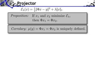
  • 36. Projector E (x) = 1 || x 2 y||2 + ||x||1 Proposition: If x1 and x2 minimize E , then x1 = x2 . Corrolary: µ(y) = x1 = x2 is uniquely defined.
  • 37. Projector E (x) = 1 || x 2 y||2 + ||x||1 Proposition: If x1 and x2 minimize E , then x1 = x2 . Corrolary: µ(y) = x1 = x2 is uniquely defined. Proof: x3 = (x1 + x2 )/2 is solution and if x1 6= x2 , 2||x3 ||1 6 ||x1 ||1 + ||x2 ||1 2|| x3 y||2 < || x1 y||2 + || x2 y||2 E (x3 ) < E (x1 ) = E (x2 ) =) contradiction.
  • 38. Projector E (x) = 1 || x 2 y||2 + ||x||1 Proposition: If x1 and x2 minimize E , then x1 = x2 . Corrolary: µ(y) = x1 = x2 is uniquely defined. Proof: x3 = (x1 + x2 )/2 is solution and if x1 6= x2 , 2||x3 ||1 6 ||x1 ||1 + ||x2 ||1 2|| x3 y||2 < || x1 y||2 + || x2 y||2 E (x3 ) < E (x1 ) = E (x2 ) =) contradiction. For (¯, ) close to (y, ) 2 H: y / µ(¯) = PI (¯) y y dI + +,⇤ = I I = I sI PI : orthogonal projector on { x supp(x) = I}.
  • 39. Overview • Polytope Noiseless Recovery • Local Behavior of Sparse Regularization • Robustness to Small Noise • Robustness to Bounded Noise • Compressed Sensing RIP Theory
  • 40. Uniqueness Sufficient Condition E (x) = 1 || x 2 y||2 + ||x||1
  • 41. Uniqueness Sufficient Condition E (x) = 1 || x 2 y||2 + ||x||1 Theorem: If I has full rank and || I c ( x y)|| < then x? is the unique minimizer of E .
  • 42. Uniqueness Sufficient Condition E (x) = 1 || x 2 y||2 + ||x||1 Theorem: If I has full rank and || I c ( x y)|| < then x? is the unique minimizer of E . Proof: Let x? be a minimizer. ˜ Then ? x = x =) ˜ ? x? ˜I x? 2 ker( I I) = {0}. || Ic ( x? ˜ y)||1 = || Ic ( x? y)||1 < =) supp(˜? ) ⇢ I x =) x? = x? ˜
  • 43. Robustness to Small Noise Identifiability crition: [Fuchs] For s ⇥ { 1, 0, +1}N , let I = supp(s) +, F(s) = || I sI || where ⇥I = Ic I ( I is assumed to have full rank) + I =( I I) 1 I satisfies + I I = IdI
  • 44. Robustness to Small Noise Identifiability crition: [Fuchs] For s ⇥ { 1, 0, +1}N , let I = supp(s) +, F(s) = || I sI || where ⇥I = Ic I ( I is assumed to have full rank) + I =( I I) 1 I satisfies + I I = IdI Theorem: If F (sign(x0 )) < 1, T = min |x0,i | i I If ||w||/T is small enough and ||w||, then x0 + + I w ( I I) 1 sign(x0,I ) is the unique solution of P (y). ⇥ If ||w|| small enough, ||x x0 || = O(||w||).
  • 45. Geometric Interpretation +, dI = sI F(s) = || I sI || = max | dI , j ⇥| I i j /I where dI defined by: dI = I( I I) 1 sI i I, dI , i = si j
  • 46. Geometric Interpretation +, dI = sI F(s) = || I sI || = max | dI , j ⇥| I i j /I where dI defined by: dI = I( I I) 1 sI i I, dI , i = si j Condition F (s) < 1: no vector j inside the cap Cs . dI j Cs i | dI , ⇥| < 1
  • 47. Geometric Interpretation +, dI = sI F(s) = || I sI || = max | dI , j ⇥| I i j /I where dI defined by: dI = I( I I) 1 sI i I, dI , i = si j Condition F (s) < 1: no vector j inside the cap Cs . dI j dI i k | dI , ⇥| < 1 j Cs i | dI , ⇥| < 1
  • 48. Sketch of Proof Local candidate: implicit equation x = x(sign(x )) ˆ where x(s)I = ˆ + I y ( I I) 1 sI , I = supp(s) ⇥ To prove: x = x(sign(x0 )) is the unique solution of P (y). ˆ ˆ
  • 49. Sketch of Proof Local candidate: implicit equation x = x(sign(x )) ˆ where x(s)I = ˆ + I y ( I I) 1 sI , I = supp(s) ⇥ To prove: x = x(sign(x0 )) is the unique solution of P (y). ˆ ˆ Sign consistency: sign(ˆ) = sign(x0 ) x (C1 ) y = x0 + w = x = x0 + ˆ + I w ( I I) 1 sI ,2 ||w|| + ||( I) + || I || I 1 || , <T = (C1 )
  • 50. Sketch of Proof Local candidate: implicit equation x = x(sign(x )) ˆ where x(s)I = ˆ + I y ( I I) 1 sI , I = supp(s) ⇥ To prove: x = x(sign(x0 )) is the unique solution of P (y). ˆ ˆ Sign consistency: sign(ˆ) = sign(x0 ) x (C1 ) y = x0 + w = x = x0 + ˆ + I w ( I I) 1 sI ,2 ||w|| + ||( I) + || I || I 1 || , <T = (C1 ) First order conditions: || Ic ( ˆ x y)|| < (C2 ) || Ic ( I + I Id)||2, ||w|| (1 F (s)) < 0 = (C2 )
  • 51. Sketch of Proof (cont) ,2 ||w|| + ||( I) + 1 || I || I || , <T = x is ˆ the solution Ic ( Id)||2, ||w|| (1 F (s)) < 0 + || I I
  • 52. Sketch of Proof (cont) ,2 ||w|| + ||( I) + 1 || I || I || , <T = x is ˆ the solution Ic ( Id)||2, ||w|| (1 F (s)) < 0 + || I I For ||w||/T < ⇥max , one can choose ||w||/T such that x is the solution of P (y). ˆ ||w|| 0 = ⇥⇤ T max | |w ||w || +⇥ ⇤= T
  • 53. Sketch of Proof (cont) ,2 ||w|| + ||( I) + 1 || I || I || , <T = x is ˆ the solution Ic ( Id)||2, ||w|| (1 F (s)) < 0 + || I I For ||w||/T < ⇥max , one can choose ||w||/T such that x is the solution of P (y). ˆ ||w|| 0 = ⇥⇤ ||ˆ x x0 || || + + ||( I I w|| I) 1 || ,2 T max = O(||w||) | |w ||w || =⇥ ||ˆ x x0 || = O(||w||) +⇥ ⇤= T
  • 54. Overview • Polytope Noiseless Recovery • Local Behavior of Sparse Regularization • Robustness to Small Noise • Robustness to Bounded Noise • Compressed Sensing RIP Theory
  • 55. Robustness to Bounded Noise Exact Recovery Criterion (ERC): [Tropp] For a support I ⇥ {0, . . . , N 1} with I full rank, ERC(I) = || I || , where ⇥I = Ic +, I = || + I Ic ||1,1 = max || c + I j ||1 j I (use ||(aj )j ||1,1 = maxj ||aj ||1 ) Relation with F criterion: ERC(I) = max F(s) s,supp(s) I
  • 56. Robustness to Bounded Noise Exact Recovery Criterion (ERC): [Tropp] For a support I ⇥ {0, . . . , N 1} with I full rank, ERC(I) = || I || , where ⇥I = Ic +, I = || + I Ic ||1,1 = max || c + I j ||1 j I (use ||(aj )j ||1,1 = maxj ||aj ||1 ) Relation with F criterion: ERC(I) = max F(s) s,supp(s) I Theorem: If ERC(supp(x0 )) < 1 and ||w||, then x is unique, satisfies supp(x ) supp(x0 ), and ||x0 x || = O(||w||)
  • 57. Sketch of Proof Restricted recovery: 1 x ⇥ argmin || x ˆ y||2 + ||x||1 supp(x) I 2 ⇥ To prove: x is the unique solution of P (y). ˆ
  • 58. Sketch of Proof Restricted recovery: 1 x ⇥ argmin || x ˆ y||2 + ||x||1 supp(x) I 2 ⇥ To prove: x is the unique solution of P (y). ˆ Implicit equation: xI = ˆ + I y ( I I) 1 sI Important: s = sign(ˆ) is not equal to sign(x ). x
  • 59. Sketch of Proof Restricted recovery: 1 x ⇥ argmin || x ˆ y||2 + ||x||1 supp(x) I 2 ⇥ To prove: x is the unique solution of P (y). ˆ Implicit equation: xI = ˆ + I y ( I I) 1 sI Important: s = sign(ˆ) is not equal to sign(x ). x First order conditions: || Ic ( ˆ x y)|| < (C2 ) || Ic ( I + I Id)||2, ||w|| (1 F (s)) < 0 = (C2 )
  • 60. Sketch of Proof Restricted recovery: 1 x ⇥ argmin || x ˆ y||2 + ||x||1 supp(x) I 2 ⇥ To prove: x is the unique solution of P (y). ˆ Implicit equation: xI = ˆ + I y ( I I) 1 sI Important: s = sign(ˆ) is not equal to sign(x ). x First order conditions: || Ic ( ˆ x y)|| < (C2 ) || Ic ( I + I Id)||2, ||w|| (1 F (s)) < 0 = (C2 ) Since s is arbitrary: ERC(I) < 1 = F (s) < 1 Hence, choosing ||w|| implies (C2 ).
  • 61. Weak ERC For A = (ai )i , B = (bi )i , where ai , bi RP , (A, B) = max | ai , bj ⇥| j i I (A) = max | ai , aj ⇥| j i=j Weak Exact Recovery Criterion: [Gribonval,Dossal] Denoting = ( i )N 1 where i=0 i RP ( I, Ic ) if ( I) <1 w-ERC(I) = 1 ( I) + otherwise. Theorem: F(s) ERC(I) w-ERC(I) (for I = supp(s))
  • 62. Proof Theorem: F(s) ERC(I) w-ERC(I) (for I = supp(s)) ERC(I) = max || + I j ||1 ||( I I) 1 ||1,1 max || I j ||1 j /I j /I max || I ⇥j ||1 = max | ⇥i , ⇥j ⇥| = ( I, Ic ) j /I j /I i m
  • 63. Proof Theorem: F(s) ERC(I) w-ERC(I) (for I = supp(s)) ERC(I) = max || + I j ||1 ||( I I) 1 ||1,1 max || I j ||1 j /I j /I max || I ⇥j ||1 = max | ⇥i , ⇥j ⇥| = ( I, Ic ) j /I j /I i m One has I I = Id H, if ||H||1,1 < 1, ( I I) 1 = (Id H) 1 = Hk k 0 1 I) = 1 ||( ||1,1 ||H||k I 1,1 1 ||H||1,1 k 0 ||H||1,1 = max | ⇥i , ⇥j ⇥| = ( I) i I j=i
  • 64. Example: Random Matrix P = 200, N = 1000 1 0.8 0.6 0.4 0.2 0 0 10 20 30 40 50 w-ERC < 1 F <1 ERC < 1 x = x0
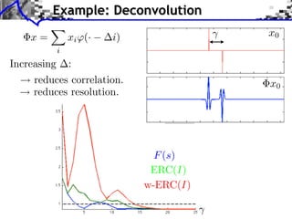
  • 65. Example: Deconvolution ⇥x = xi (· i) x0 i Increasing : reduces correlation. x0 reduces resolution. F (s) ERC(I) w-ERC(I)
  • 66. Coherence Bounds Mutual coherence: µ( ) = max | i, j ⇥| i=j |I|µ( ) Theorem: F(s) ERC(I) w-ERC(I) 1 (|I| 1)µ( )
  • 67. Coherence Bounds Mutual coherence: µ( ) = max | i, j ⇥| i=j |I|µ( ) Theorem: F(s) ERC(I) w-ERC(I) 1 (|I| 1)µ( ) 1 1 Theorem: If ||x0 ||0 < 1+ and ||w||, 2 µ( ) one has supp(x ) I, and ||x0 x || = O(||w||)
  • 68. Coherence Bounds Mutual coherence: µ( ) = max | i, j ⇥| i=j |I|µ( ) Theorem: F(s) ERC(I) w-ERC(I) 1 (|I| 1)µ( ) 1 1 Theorem: If ||x0 ||0 < 1+ and ||w||, 2 µ( ) one has supp(x ) I, and ||x0 x || = O(||w||) N P One has: µ( ) P (N 1) Optimistic setting: For Gaussian matrices: ||x0 ||0 O( P ) µ( ) log(P N )/P For convolution matrices: useless criterion.
  • 69. Coherence - Examples Incoherent pair of orthobases: Diracs/Fourier 2i 1 = {k ⇤⇥ [k m]}m 2 = k N 1/2 e N mk m =[ 1, 2] RN 2N
  • 70. Coherence - Examples Incoherent pair of orthobases: Diracs/Fourier 2i 1 = {k ⇤⇥ [k m]}m 2 = k N 1/2 e N mk m =[ 1, 2] RN 2N 1 min ||y x||2 + ||x||1 x R2N 2 1 min ||y 1 x1 2 x2 ||2 + ||x1 ||1 + ||x2 ||1 x1 ,x2 RN 2 = +
  • 71. Coherence - Examples Incoherent pair of orthobases: Diracs/Fourier 2i 1 = {k ⇤⇥ [k m]}m 2 = k N 1/2 e N mk m =[ 1, 2] RN 2N 1 min ||y x||2 + ||x||1 x R2N 2 1 min ||y 1 x1 2 x2 ||2 + ||x1 ||1 + ||x2 ||1 x1 ,x2 RN 2 = + 1 µ( ) = = separates up to N /2 Diracs + sines. N
  • 72. Overview • Polytope Noiseless Recovery • Local Behavior of Sparse Regularization • Robustness to Small Noise • Robustness to Bounded Noise • Compressed Sensing RIP Theory
  • 73. CS with RIP 1 recovery: y = x0 + w x⇥ argmin ||x||1 where || x y|| ||w|| 1 ⇥ argmin || x y||2 + ||x||1 x 2 Restricted Isometry Constants: ⇥ ||x||0 k, (1 k )||x||2 || x||2 (1 + k )||x||2
  • 74. CS with RIP 1 recovery: y = x0 + w x⇥ argmin ||x||1 where || x y|| ||w|| 1 ⇥ argmin || x y||2 + ||x||1 x 2 Restricted Isometry Constants: ⇥ ||x||0 k, (1 k )||x||2 || x||2 (1 + k )||x||2 Theorem: If 2k 2 1, then [Candes 2009] C0 ||x0 x || ⇥ ||x0 xk ||1 + C1 k where xk is the best k-term approximation of x0 .
  • 75. Elements of Proof Reference: E. J. Cand`s, CRAS, 2006 e k elements {0, . . . , N 1} = T0 ⇥ T1 ⇥ . . . ⇥ Tm h=x x0 largest largest xk = xT0 of x0 of hT0c Optimality conditions: ||hT0 ||1 c ||hT0 ||1 + 2||xT0 ||1 c Explicit constants: 2 2k C0 = ||x0 x || ⇥ ||x0 xk ||1 + C1 1 2k s 1 + 2k 2 =2 C0 = C1 = 1 1 1 ⇥ 2k
  • 76. Singular Values Distributions Eigenvalues of I I with |I| = k are essentially in [a, b] a = (1 )2 and b = (1 )2 where = k/P When k = P + , the eigenvalue distribution tends to 1 f (⇥) = (⇥ b)+ (a ⇥)+ [Marcenko-Pastur] 1.5 2⇤ ⇥ P=200, k=10 P=200, k=10 f ( ) 1.5 1 1 0.5 P = 200, k = 10 0.5 0 0 0.5 1 1.5 2 2.5 0 0 0.5 1 P=200, k=30 1.5 2 2.5 1 P=200, k=30 0.8 1 0.6 0.8 0.4 k = 30 0.6 0.2 0.4 0 0.2 0 0.5 1 1.5 2 2.5 0 0 0.5 1 P=200, k=50 1.5 2 2.5 P=200, k=50 0.8 0.8 0.6 0.6 0.4 Large deviation inequality [Ledoux] 0.4 0.2
  • 77. RIP for Gaussian Matrices Link with coherence: µ( ) = max | i, j ⇥| i=j 2 = µ( ) k (k 1)µ( )
  • 78. RIP for Gaussian Matrices Link with coherence: µ( ) = max | i, j ⇥| i=j 2 = µ( ) k (k 1)µ( ) For Gaussian matrices: µ( ) log(P N )/P
  • 79. RIP for Gaussian Matrices Link with coherence: µ( ) = max | i, j ⇥| i=j 2 = µ( ) k (k 1)µ( ) For Gaussian matrices: µ( ) log(P N )/P Stronger result: C Theorem: If k P log(N/P ) then 2k 2 1 with high probability.
  • 80. Numerics with RIP Stability constant of A: (1 ⇥1 (A))|| ||2 ||A ||2 (1 + ⇥2 (A))|| ||2 smallest / largest eigenvalues of A A
  • 81. Numerics with RIP Stability constant of A: (1 ⇥1 (A))|| ||2 ||A ||2 (1 + ⇥2 (A))|| ||2 smallest / largest eigenvalues of A A Upper/lower RIC: i k = max i( I) ˆ2 |I|=k k k = min( k , 1 k) 2 2 1 ˆ2 k Monte-Carlo estimation: ˆk k k
  • 82. Conclusion s=3 s=6 Local behavior: 0.5 0.5 ! x? polygonal. 0 ? 0 y ! x piecewise a ne. −0.5 −0.5 −1 10 20 30 40 50 60 10 20 30 40 50 60 s=13 s=25 1 1.5 1 0.5 0.5 0 0 −0.5 −0.5 −1 −1.5 20 40 60 80 100 20 40 60 80 100 120 140
  • 83. Conclusion s=3 s=6 Local behavior: 0.5 0.5 ! x? polygonal. 0 ? 0 y ! x piecewise a ne. −0.5 −0.5 Noiseless recovery: −1 10 20 30 40 50 60 10 20 30 40 50 60 () geometry of polytopes. s=13 s=25 1 1.5 1 0.5 0.5 0 0 −0.5 x0 −0.5 −1 −1.5 20 40 60 80 100 20 40 60 80 100 120 140
  • 84. Conclusion s=3 s=6 Local behavior: 0.5 0.5 ! x? polygonal. 0 ? 0 y ! x piecewise a ne. −0.5 −0.5 Noiseless recovery: −1 10 20 30 40 50 60 10 20 30 40 50 60 () geometry of polytopes. s=13 s=25 Small noise: 1 1.5 1 ! sign stability. 0.5 0.5 0 Bounded noise: 0 −0.5 x0 −0.5 −1 ! support inclusion. −1.5 20 40 60 80 100 20 40 60 80 100 120 140 RIP-based: ! no support stability, L1 bounds.