Software Metrics Course chapter 5 at Bahir Dar University

Course Name:-Software Metrics
Chapter 5:
Measuring Internal
Product Attributes:
Software Size
compiled by Samuel Ashagrre
SOFTWARE METRICS 1

Contents
► Software size
► Size: Length (code, specification, design)
► Size: Reuse
► Size: Functionality (function point, feature
point, object point, use-case point)
► Size: Complexity

Software Size
4
• Software size can be described with three such
attributes:
– Length
– Functionality
– Complexity
• Length is the physical size of the product, and
• Functionality measures the functions supplied by
the product to the user.
• Complexity can be interpreted in different ways.
5

Different types of Complexity
5
• Problem complexity (also called computational complexity)
measures the complexity of the underlying problem.
• Algorithmic complexity reflects the complexity of the
algorithm implemented to solve the problem; in some sense,
this type of complexity measures the efficiency of the
software.
• Structural complexity measures the structure of the
software used to implement the algorithm.
– For example, we look at control flow structure, hierarchical structure
and modular structure to extract this type of measure.
• Cognitive complexity measures the effort required to
understand the software
7
CAPS

Software Size
■ Internal product attributes describe a software
product in a way that is dependent only on the
product itself.
■ One of the most useful attributes is the size of a
sofware product, which can be measured statically,
i.e., without executing the system.
■ Size measurement must reflect effort, cost and
productivity.

Software Size: Length
■ Length is the “physical size” of the product.
■ In a software development effort, there are three
major development products: specification, design,
and code.
■ The length of the specification can indicate how
long the design is likely to be, which in turn is a
predictor of code length.
■ Traditionally, code length refers to text-based code
length.

Length- Code
8
Traditional code measures
•The most commonly used measure of source code
program length is the number of lines of code (LOC),
•But one set of lines of code are different from others.
– For example, many programmers use spacing and blank
lines to make their programs easier to read.
– If lines of code are being used to estimate programming
effort, then a blank line does not contribute the same
amount of effort.
– Similarly, comment lines improve a program's
understandability, and they certainly require some effort to
write.
– But they may not require as much effort as the code itself
13

Length: Code - LOC
■ The most commonly used measure of source code
program length is the number of lines of code (LOC).
■ NCLOC: non-commented source line of code or
effective lines of code (ELOC).
■ CLOC: commented source line of code.
■ By measuring NCLOC and CLOC separately we
can define:
total length (LOC) = NCLOC + CLOC
■ The ratio: CLOC/LOC measures the density of
comments in a program.

Length: Code - LOC (cont.)
The SLOC values for various operating systems in
Microsofts Windows NT product line are as follows:

System size
What is a large project?
• JavaScript project sizes are typically classified
based on the number of lines of code (LOC) or
complexity of the application.
• Here’s a general classification:

 Small Projects:
Description: These are simple scripts or applications
with limited functionality.
Examples: Form validation, basic DOM manipulation,
single-function widgets.
Lines of Code: Typically less than 1,000 LOC.
Team: Usually handled by one developer.

 Medium Projects
Description: Applications with moderate complexity,
such as standalone front-end web apps or moderately
interactive websites.
Examples: Portfolio websites, small e-commerce stores,
or single-page applications (SPAs) with limited backend
integration.
Lines of Code: Between 1,000 and 10,000 LOC.
Team: Small team of 2-5 developers.

 Large Projects
Description: Complex applications that require robust
architecture, frameworks, and team collaboration.
Examples: Enterprise-level web applications, advanced
SPAs with backend API integration, or cross-platform
apps using frameworks like React or Vue.
Lines of Code: Between 10,000 and 100,000 LOC.
Team: Teams of 5-20 developers with specialized roles
(e.g., frontend, backend, UI/UX).

 Very Large Projects
Description: Highly complex systems or ecosystems of
interdependent services and applications.
Examples: Large-scale social media platforms, cloud
dashboards, video streaming services, or SaaS platforms.
Lines of Code: 100,000+ LOC.
Team: Multiple teams across departments, often 20+
developers.

■
Advantages of LOC
■ Simple and automatically measurable
■ Correlates with programming effort (& cost)
■ Disadvantage of LOC
Vague definition
Language dependability
Not available for early planning
Developers’ skill dependability
■
■
■
■

Length: Halstead’s Work
■ Maurice Halstead’s Theory (1971~1979):
■ A program P is a collection of tokens, composed of
two basic elements: operands and operators
Operands are variables, constants, addresses
Operators are defined operations in a
programming language
■
■
(language constructs) a, b, x
100
if ... else + - >
= main()
goto

Halstead's Software Science
19
• The logic of Halstead’s software science is that
“any programming task consists of selecting and
arranging a finite number of program "tokens,"
which are basic syntactic units distinguishable by
a compiler.”
• A computer program, according to software
science, is a collection of tokens that can be
classified as either operators or operands.

20
• Based on these primitive measures, Halstead
developed a system of equations expressing
– total vocabulary,
The total number of unique operator and unique
operand occurrences.

21
– overall program length
The total number of operator occurrences and the
total number of operand occurrences.

22
– program difficulty
This parameter shows how difficult to handle the
program is.
As the volume of the implementation of a program
increases, the program level decreases and the
difficulty increases.
Thus, programming practices such as redundant
usage of operands, or the failure to use higher-
level control constructs will tend to increase the
volume as well as the difficulty.

23
– Programming Effort – Measures the amount of
mental activity needed to translate the existing
algorithm into implementation in the specified
program language.
– Language Level – Shows the algorithm
implementation program language level.
– The same algorithm demands additional effort if
it is written in a low-level program language. For
example, it is easier to program in Pascal than in
Assembler.

24
– program level (a measure of software complexity),
To rank the programming languages, the level of
abstraction provided by the programming
language, Program Level (L) is considered.
The higher the level of a language, the less effort it
takes to develop a program using that language.
The value of L ranges between zero and one, with L=1 representing a program
written at the highest possible level

25
– Intelligence Content – Determines the amount
of intelligence presented (stated) in the program
This parameter provides a measurement of
program complexity, independently of the program
language in which it was implemented.

26
– Programming Time – Shows time (in minutes)
needed to translate the existing algorithm into
implementation in the specified program language.

Length: Halstead’s Work /2
The basic metrics for these tokens are the following
 Number of distinct operators in the program (µ1)
 Number of distinct operands in the program (µ2)
 Total number of occurrences of operators in the
program (N1)
 Total number of occurrences of operands in the
program (N2)
Program vocabulary (µ)
µ = µ1 + µ2

Software Metrics Course chapter 5 at Bahir Dar University

 Program Difficulty – This parameter shows how
difficult to handle the program is.
D = (µ1 / 2) * (N2 / µ2)
D = 1 / L
As the volume of the implementation of a program
increases, the program level decreases and the difficulty
increases.
Thus, programming practices such as redundant usage
of operands, or the failure to use higher-level control
constructs will tend to increase the volume as well as
the difficulty.

 Intelligence Content – Determines the amount of
intelligence presented (stated) in the program
 This parameter provides a measurement of program
complexity, independently of the program language
in which it was implemented.
I = V / D

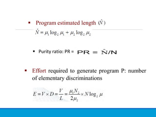
 Program estimated length
 Effort required to generate program P: number
of elementary discriminations
 Purity ratio: PR =

 Time required for developing program P is the total
effort divided by the number of elementary
discriminations per second
 In cognitive psychology β is usually a number
between 5 and 20
 Halstead claims that β =18

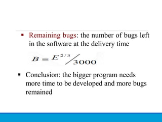
 Remaining bugs: the number of bugs left
in the software at the delivery time
 Conclusion: the bigger program needs
more time to be developed and more bugs
remained

Counting rules for C language/1
 Comments are not considered.
 All the variables and constants are considered
operands.
 Global variables used in different modules of
the same program are counted as multiple
occurrences of the same variable.
 Local variables with the same name in different
functions are counted as unique operands.
 Functions calls are considered as operators.

Counting rules for C language /2
 All looping statements e.g., do {…} while ( ),
while ( ) {…}, for ( ) {…}, all control statements
e.g., if ( ) {…}, if ( ) {…} else {…}, etc. are
considered as operators.
 In control construct switch ( ) {case:…}, switch as
well as all the case statements are considered as
operators.

 The reserve words like return, default, continue,
break, sizeof, etc., are considered as operators.
 All the brackets, commas, and terminators are
considered as operators.
 GOTO is counted as an operator and the label is
counted as an operand.

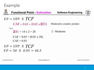
 The unary and binary occurrence of “+” and “-”
are dealt separately. Similarly “*” (multiplication
operator) are dealt separately.
 In the array variables such as “array-name
[index]” “array-name” and “index” are
considered as operands and [ ] is considered as
operator.

 In the structure variables such as “struct-name,
member-name” or “struct-name -> member-
name”, struct-name, member-name are taken as
operands and ‘.’, ‘->’ are taken as operators.
 Some names of member elements in different
structure variables are counted as unique
operands.
 All the hash directive are ignored.

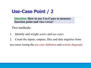
List out the operators and operands and also calculate
the values of software science measures like
int sort (int x[ ], int n)
{
int i, j, save, im1;
/*This function sorts array x in ascending order */
If (n< 2) return 1;
for (i=2; i< =n; i++)
{
im1=i-1;
for (j=1; j< =im1; j++)
if (x[i] < x[j])
{
Save = x[i];
x[i] = x[j];
x[j] = save;
}
}
return 0;
}

List out the operators and operands and also calculate
the values of software science measures like

Result:
μ1 = 14
N1 = 53
μ2=10
N2=38

Result:
Therefore, N = 91
μ = 24
V = ?
N^ = ?
V* = ?
L = ?
D = ?
T = ?

Exercise 1:determine the 10 software science measures for the following
program
def factorial(n):
if n == 0:
return 1
else:
result = 1
for i in range(1, n + 1):
result *= i
return result

Tools for Complex Code:
For analyzing large projects, consider using automated tools like:
• SonarQube:
• Provides detailed complexity and maintainability reports.

• Radon (Python-specific): Computes Halstead complexity and
other metrics.
• McCabe’s complexity, i.e. cyclomatic complexity
• raw metrics (these include SLOC, comment lines, blank
lines, &c.)
• Halstead metrics (all of them)
• Maintainability Index (the one used in Visual Studio)
• Installation
• With Pip:
• $ pip install radon

Cyclomatic Complexity Example

Critics of Halstead’s work
Developed in the context of assembly languages and too
fine grained for modern programming languages.
The treatment of basic and derived measures is
somehow confusing.
The notions of time to develop and remaining bugs are
arguable.
Unable to be extended to include the size for
specification and design.
•It depends on usage of operator and operands in
completed code.
•It has no use in predicting complexity of program at
design level.

Advantages of Halstead
49
•Do not require in-depth and control flow analysis
of program.
•Predicts Effort, rate of error and time.
•Useful in scheduling projects.

Length: Alternative Methods
 Alternative methods for text-based measurement of
code length:
1) Source memory size: Measuring length in terms of
number of bytes of computer storage required for the
program text. Excludes library code.
2) Char size: Measuring length in terms of number
of characters (CHAR) in program text.
3) Object memory size: Measuring length in terms of an
object (executable or binary) file. Includes library code.
 All are relatively easy to measure (or estimate).
SOC

Length: Code - Problems /1
 One of the problems with text-based definition of length
is that the line of code measurement is increasingly less
meaningful as software development turns to more
automated tools, such as:
 Tools that generate code from specifications
 Visual programming tools

Code Length in OOP
Object-oriented development also suggests new ways to
measure length.
Pfleeger found that a count of objects and methods led
to more accurate productivity estimates than those using
lines of code
52

Code Length in OOP
Lorenz found in his research at IBM that the average
class contained 20 methods, and the average method size
was 8 lines of code for Smalltalk and 24 for C++.
He also notes that size differs with system and
application type.
53

Importance of Reuse in Size
This reuse of software (including requirements, designs,
documentation, and test data and scripts as well as code)
◦ improves our productivity and quality,
◦ allows us to concentrate on new problems, rather than
continuing to solve old ones again.
54

NASA/Goddard's Software Engineering Laboratory
◦ Reused verbatim: the code in the unit which was
reused without any changes.
◦Slightly modified: fewer that 25% of the lines of code
in the unit were modified.
◦ Extensively modified: 25% or more of the lines of
code were modified.
◦ New: none of the code comes from a previously
constructed unit.
55

NASA/Goddard's Software Engineering Laboratory
56

Hewlett-Packard considers three levels of code:
◦new code, reused code, and leveraged code.
reused code is used as is, without modification,
leveraged code is existing code that is modified in some
way.
The Hewlett-Packard reuse ratio includes both reused
and leveraged code as a percentage of total code
delivered.
57

Measuring Software Size:
 Function Point (FP),
 Feature Point,
 Object Point and
 Use-case Point

Function-Oriented Metrics
 Function Point (FP) is a weighted measure of
software functionality.
 The idea is that a product with more functionality will
be larger in size.
 Function-oriented metrics are indirect measures of
software which focus on functionality and utility.
 The first function-oriented metrics was proposed by
Albrecht (1979~1983) who suggested a productivity
measurement approach called the Function Point (FP) method.
 Function points (FPs) measure the amount of functionality
in a system based upon the system specification.
 Estimation before implementation!

Function Points(FP) can be used to size software
applications accurately
FP are becoming widely accepted as the standard metric
for measuring software size
FP have made adequate sizing possible.
Without a reliable sizing metric relative changes in
productivity or relative changes in quality can not be
calculated.
61

Keywords
•Function Point: is a unit of measure for quantifying software
deliverable (functionality) based upon the user view.
•User: is any person or thing that communicates or interacts with
the software at any time
•User View : is the Functional User Requirements as perceived by
the user.
•Functional user requirements : are a subset of user requirements,
that describe what the software shall do (functions), in terms of
tasks and services
62

Calculating Function Points
63

64
Determine the number of components (EI, EO, EQ, ILF, and ELF)
EI −The number of external inputs. These are
elementary processes in which derived data passes
across the boundary from outside to inside.
receives information from outside the application
boundary,
 In an example library database system, enter an
existing patron's library card number.
EO −The number of external output. These are
elementary processes in which derived data passes
across the boundary from inside to outside.
presents information of the information system,
In an example library database system, display a list
of books checked out to a patron.
.

65
EQ − The number of external queries. These are elementary
processes with both input and output components that result
in data retrieval from one or more internal logical files and
external interface files.
In an example library database system, determine what
books are currently checked out to a patron.
ILF − The number of internal logical files.
contains permanent data that is relevant to the user The
information system references and maintains the data
These are user identifiable groups of logically related data that
resides entirely within the applications boundary that are
maintained through external inputs.
In an example library database system, the file of books
in the library.

66
ELF − The number of external log files. These are user
identifiable groups of logically related data that are used
for reference purposes only, and which reside entirely
outside the system.
 In an example library database system, the file that
contains transactions in the library's billing system.
also contains permanent data that is relevant to the
user. The information system references the data,
but the data is maintained by another information
system

FP: Advantages - Summary
This FP can then be used in various metrics, such as:
Cost = $ / FP
Quality = Errors / FP
Productivity = FP / person-month

FP: Advantages - Summary
 Can be counted before design or code documents exist
 Can be used for estimating project cost, effort, schedule
early in the project life-cycle
 Helps with contract negotiations
 Is standardized (though several competing standards exist)
 It is independent of the programming language,
technology, techniques.

"Guesstimate" Instead of Estimate!
 FP is a subjective measure: affected by the selection of
weights by external users.
 Function point calculation requires a full software
system specification. It is therefore difficult to use
function points very early in the software development
lifecycle.
 Physical meaning of the basic unit of FP is unclear.
 Unable to account for new versions of I/O, such as
data streams, intelligent message passing, etc.
 Not suitable for “complex” software, e.g., real-time and
embedded applications.

Extended Function Point (EFP) Metrics
■ FP metric has been further extended to
compute:
A. Feature points.
B. 3D function points.

Feature Point /1
■ Function points were originally designed to be applied
to business information systems. Extensions have been
suggested called feature points which may enable this
measure to be applied to other software engineering
applications.
■ Feature points accommodate applications in which the
“algorithmic complexity” is high such as real-time, process
control, and embedded software applications.
■ For conventional software and information systems
functions and feature points produce similar results. For
complex systems, feature points often produce counts about
%20~%35 higher than function points.

Feature Point 12
■ Feature points are calculated the same way as FPs
with the additions of algorithms as an additional
software characteristic.
■ Counts are made for the five FP categories, i.e.,
number of external inputs, external outputs,
inquiries, internal files, external interfaces, plus:
■ Algorithm (Na): A bounded computational problem such as
inverting a matrix, decoding a bit string, or handling an
interrupt.

Example
• Given Components: calculate Function Points (FP) and Feature Points (FPT) from the same data
Component Count Complexity Weight (FP) Weight (FPT)
Internal
Logical Files
(ILF)
3 Average 10 10
External
Interface Files
(EIF)
2 Low 5 5
External
Inputs (EI)
10 Average 4 4
External
Outputs (EO)
5 High 7 7
External
Inquiries (EQ)
3 Low 3 3
Algorithmic
Complexity
(AC)**
(Feature
Points Only)
5 N/A 5

Example
• Function Point (FP) Calculation
• Step 1: Calculate Unadjusted Function Points
(UFP)Using FP weights:
• UFP=(3×10)+(2×5)+(10×4)+(5×7)+(3×3)
• UFP=30+10+40+35+9=124

Example
• Function Point (FP) Calculation cont..
• Step 2: Adjust for Complexity
• Assume the General System Characteristics
(GSC) score = 30.
• Complexity Adjustment Factor
(CAF)=0.65+(0.01×30)=0.95
• Step 3: Calculate Final Function Points
• FP=UFP×CAF=124×0.95=117.8

Example
• Feature Point (FPT) Calculation
• Step 1: Calculate Unadjusted Feature Points
• Feature Points include all Function Point
components, plus Algorithmic Complexity (AC).
Using FPT weights:
• UFPFPT=(3×10)+(2×5)+(10×4)+(5×7)+(3×3)+(5×5)UFP FPT
=(3×10)+(2×5)+(10×4)+(5×7)+(3×3)+(5×5)UFPFPT=30+10+40+35
+9+25=149UFP FPT =30+10+40+35+9+25=149

Example
• Feature Point (FPT) Calculation cont..
• Step 2: Adjust for Complexity
• Assume the same GSC score =30.
• CAF=0.65+(0.01×30)=0.95
• Step 3: Calculate Final Feature Points
• FPT=UFPFPT×CAF=149×0.95=141.55

Exercise
Scenario: E-commerce System
Elements Identified:
External Inputs: Add item, Update item (2 average).
External Outputs: Generate invoice, Display summary (2
complex).
External Inquiries: Search product (1 simple).
Internal Files: Inventory, Order history (2 average).
External Interfaces: Payment gateway (1 complex).
Complex Processing: Real-time inventory updates (1
complex).

Object Point /1
 Object points are used as an initial measure for size way
early in the development cycle, during feasibility studies.
 An initial size measure is determined by counting the
number of screens, reports, and third-generation components
that will be used in the application.
 Each object is classified as simple, medium, or difficult.

Object Point /2
 are used in software development to estimate the
size and complexity of a project, particularly for
systems designed with object-oriented or visual
programming environments.
 These metrics focus on user-visible objects rather
than traditional lines of code (LOC) or functional
units.

Object Point /3
Key Components of Object Point Metrics
 Screens: Refers to user interface components or visual
elements used to display information or gather user input.
 Examples: Data entry forms, dashboards.Reports:
 Output elements designed to display or summarize data for
users.
 Examples: Financial summaries, activity logs.
 3GL Components:
 Custom modules or scripts written in third-generation
programming languages (3GL), such as Java, C++, or
Python.

Object Point /5
Calculation Steps for Object Point Metrics
1. Count Object Types
Determine the number of screens, reports, and 3GL
components in the system.
2. Classify Complexity
Classify each object as simple, medium, or difficult based on
factors like functionality and interactivity:
Simple: Few data items or minimal interaction.
Medium: Moderate data or interactivity.
Difficult: Complex logic or large data volume.
3. Assign Weights
Assign a weight to each object based on its type and
complexity. Typical weights might look like this:

Object Point /6
Calculation Steps for Object Point Metrics
4. Calculate Unadjusted Object Points (UOP)
• Multiply the count of each object type by its weight and
sum the results:
• UOP=∑(Count×Weight)
5. Adjust for Complexity
• Apply an Environmental Factor adjustment to account for
technical and environmental considerations, such as team
expertise or tool availability:
• Adjusted Object Points=UOP × Adjustment Factor
• The adjustment factor typically ranges from 0.7 (low
complexity) to 1.3 (high complexity).

Object Point /7
Example Calculation
Given Data:
Screens: 5 simple, 3 medium, 2 difficult.
Reports: 4 simple, 2 medium.
3GL Components: 2 medium, 1 difficult.

Object Point /8
Example Calculation
Step 1:
Calculate UOP:
• Screens=(5×1.0)+(3×2.0)+(2×3.0)=5+6+6=17
• Reports=(4×2.0)+(2×3.0)=8+6=14
• 3GL Components=(2×6.0)+(1×10.0)=12+10=22
• UOP=17+14+22=53
Step 2: Apply Adjustment Factor:
• Assume the adjustment factor is 1.2 (medium complexity).
Adjusted Object Points=53×1.2=63.6

Use-Case Point
• widely used software estimation method,
particularly effective for object-oriented systems.
• It estimates the effort required to develop
software by analyzing the complexity of use cases
and the associated system/environmental
factors.

Use-Case Point /1
 Function Point is a method to measure
software size from a requirements
perspective.
 Use-Case is a method to develop
requirements. Use Cases are used to
validate a proposed design and to ensure it
meets all requirements.
Question: How to use Use-Cases to measure
function point and vice-versa?

Use-Case Point / 2
Question: How to use Use-Cases to measure
function point and vice-versa?
Two methods:
1. Identify and weight actors and use-cases
2. Count the inputs, outputs, files and data inquiries from
use-cases (using the use-case definition and activity diagram).

Steps to Calculate UCP
120
1. Identify Use Cases and Actors
Use Cases: Functionalities of the system described from
an end-user perspective.
Actors: Entities interacting with the system (e.g., users,
external systems).

121
2. Classify and Weight Use Cases and Actors
Assign a complexity level (Simple, Average, or Complex)
and corresponding weight.
Weights for Use Cases:
Simple: 5 points
Average: 10 points
Complex: 15 points
Weights for Actors:
Simple (System with a defined API): 1 point
Average (Interactive or command-line): 2 points
Complex (Graphical UI or another system): 3 points

122
3. Calculate Unadjusted Use Case Points (UUCP)
Unadjusted Actor Weight (UAW) = Sum of all actor
weights.
Unadjusted Use Case Weight (UUCW) = Sum of all use
case weights.
UUCP = UAW + UUCW.

123
4. Adjust for Technical and Environmental Factors
Evaluate Technical Complexity Factors (TCF) and
Environmental Factors (EF).
Technical Complexity Factors: (13 factors, such as
performance, security, reusability)

124
List of the 13 Technical Complexity Factors
T1: Distributed system
T2: Performance objectives
T3: End-user efficiency
T4: Complex internal processing
T5: Reusability
T6: Easy to install
T7: Easy to use
T8: Portable

125
List of the 13 Technical Complexity Factors
T9: Easy to change
T10: Concurrent use
T11: Security features
T12: Access for third parties
T13: Special training needs

126
4. Adjust for Technical and Environmental Factors
Example formula:
TCF=0.6+(0.01×Sum of T-factor ratings)
Environmental Factors: (8 factors, like team experience
and tools availability)
Example formula:
EF=1.4−(0.03×Sum of E-factor ratings)

127
8 Factors of ECF:
1. Team Experience:
•How experienced the development team is with the technology
and domain of the project.
•Teams with more experience are generally more efficient.
Rating:
0 = Very inexperienced team
1 = Less experienced team5
= Highly experienced team

128
8 Factors of ECF:
2. Application Experience::
• The team's experience with the specific application type or
domain. If the team has worked on similar systems before, the
project will be easier to develop.
Rating:
0 = No prior experience
1 = Little prior experience
5 = Extensive prior experience

129
8 Factors of ECF:
3. Motivation of the Team
• The level of motivation and morale within the team. A highly
motivated team tends to be more productive and delivers better
results.
Rating:
0 = Very low motivation
1 = Low motivation
5 = High motivation

130
8 Factors of ECF:
4. Performance Constraints:
• How strict the performance requirements are. If the system
has strict performance needs (e.g., response time, throughput),
it will increase complexity.
Rating:
0 = No performance constraints
1 = Some constraints
5 = Very strict performance constraints

131
8 Factors of ECF:
5. Security Requirements:
• The level of security required by the system. More stringent
security requirements can complicate design and
implementation.
Rating:
0 = No security requirements
1 = Basic security requirements
5 = Very high security requirements

132
8 Factors of ECF:
5. Technical Complexity:
• The technical complexity of the system, including the need for
advanced algorithms, integration with other systems, or cutting-
edge technology. More complex systems require more effort.
Rating:
0 = Low technical complexity
1 = Moderate technical complexity
5 = High technical complexity

133
8 Factors of ECF:
6. Tool Support:
• The quality and availability of tools, frameworks, and
platforms used during development. Good tool support (such as
modern IDEs, code libraries, or automation tools) can reduce
effort.
Rating:
0 = No tool support
1 = Poor tool support
5 = Excellent tool support

134
8 Factors of ECF:
8. Development Environment
• The overall quality of the development environment,
including whether the team has a conducive working
environment, proper infrastructure, and necessary resources
(e.g., hardware, software, network).
Rating:
0 = Poor development environment
1 = Average development environment
5 = Excellent development environment

135
8 Factors of ECF:
• To calculate the ECF, each of the 8 factors is given a rating
between 0 and 5, based on the specific project environment. The
ratings for each factor are then summed up, and the total score
is used to determine the ECF value.
•Sum the Ratings: Add the ratings for all 8 factors. The maximum
possible sum is 40 (if each factor gets a rating of 5).
•Calculate the ECF: The ECF value is calculated using the formula:

Example of ECF Calculation
136
Let’s say we’re working on a system with the following factor
ratings:
•Team Experience: 4 (Experienced team)
•Application Experience: 3 (Some experience)
•Motivation of the Team: 5 (Highly motivated)
•Performance Constraints: 4 (Some performance constraints)
•Security Requirements: 2 (Basic security)
•Technical Complexity: 3 (Moderate complexity)
•Tool Support: 4 (Good tool support)
•Development Environment: 4 (Good working environment)

Example of ECF Calculation
137
•The sum of the ratings
is:4+3+5+4+2+3+4+4=294+3+5+4+2+3+4+4=29
•Using the formula:
•𝐸𝐶𝐹=0.65+(29/100)=0.65+0.29=0.94
•So, the ECF value is 0.94.
•Once the ECF is calculated, it is used to adjust the Use Case
Points (UCP) based on the environmental complexity.

138
5. Calculate Final Use Case Points
Adjusted Use Case Points (UCP) = UUCP × TCF × EF.
6. Estimate Effort
Determine a productivity factor (e.g., 20 hours per
UCP) to estimate total development time.
Effort (Hours)=UCP × Productivity Factor.

Exercise
139
Step 1: Identify Use Cases
Login (simple)
Browse Products (average)
Place Order (complex)
Check Order Status (average)

Exercise
140
Step 2: Classify Use Cases by Complexity
Login: Simple → 5 points
Browse Products: Average → 10 points
Place Order: Complex → 15 points
Check Order Status: Average → 10 points

Exercise
141
Step 3: Identify and Classify Actors
We also have the following actors:
Customer (simple)
Admin (average)
Payment Gateway (complex)

Exercise
142
Step 4: Assign Weights to Actors
Customer: Simple → 1 point
Admin: Average → 2 points
Payment Gateway: Complex → 3 points

Exercise
143
Step 5: Calculate Unadjusted Use Case Points (UCP)
Sum of Use Case Points:5+10+15+10=40 points
Sum of Actor Points:1+2+3=6 points

Exercise
144
Step 6: Calculate Technical Complexity Factor (TCF)
Assume we have the following ratings for the 13
technical factors:
For simplicity, let’s assume the total technical
complexity rating is 60 out of 100.

Exercise
145
The TCF would then be:
𝑇𝐶𝐹=0.6 (assuming the scale is between 0.5 and 1.0, wi
th the value derived from technical ratings)
Step 7: Calculate Environmental Complexity Factor
(ECF)
Assume the following environmental complexity:
The development environment is considered
moderately complex with a rating of 4 out of 5.

Exercise
146
The ECF would be:
ECF=1.2(again, based on ratings and scaled to the 0.5–
1.5 range)
Step 8: Calculate Final Use Case Points (UCP)
Now, we can calculate the final Use Case
Points:𝑈𝐶𝑃=(40+6)×0.6×1.2=46×0.6×1.2=33.12 UCP≈33 UCP

Complexity
The complexity of a solution can be regarded in
terms of the resources needed to implement a particular
solution.
We can view solution complexity as having at least two
aspects:
◦time complexity: where the resource is computer time
◦ space complexity: where the resource is computer
memory.
147

Time Complexity
◦Time Complexity is a way to represent the amount of time needed
by the program to run till its completion.
◦Time Complexity is most commonly estimated by counting the
number of elementary functions performed by the algorithm.
◦And since the algorithm's performance may vary with different
types of input data, hence for an algorithm we usually use the
worst-case Time complexity of an algorithm because that is the
maximum time taken for any input size.
148

Space Complexity
◦Its the amount of memory space required by the algorithm, during
the course of its execution.
◦An algorithm generally requires space for following components :
◦Instruction Space : Its the space required to store the executable
version of the program. This space is fixed, but varies depending
upon the number of lines of code in the program.
◦Data Space : Its the space required to store all the constants and
variables value.
◦Environment Space : Its the space required to store the
environment information needed to resume the suspended
function.
149

 To compare the efficiency of algorithms, a measure of
the degree of difficulty of an algorithm called
computational complexity.
Computational complexity indicates how much effort
is needed to execute an algorithm, or what its cost is.
This cost can be expressed in terms of execution time
(time efficiency, the most common factor) or memory
(space efficiency).
150

Software Metrics Course chapter 5 at Bahir Dar University

More Related Content

Similar to Software Metrics Course chapter 5 at Bahir Dar University (20)

More from ethiobahirdarhotel (6)

Recently uploaded (20)

Software Metrics Course chapter 5 at Bahir Dar University