Solving High-order Non-linear Partial Differential Equations by Modified q-Homotopy Analysis Method
0 likes46 views

The paper introduces the modified q-homotopy analysis method (mq-ham) for solving high-order non-linear partial differential equations, improving convergence and accuracy over previous methods. The authors demonstrate the effectiveness of mq-ham through illustrative examples, specifically addressing the second- and third-order cases. Overall, mq-ham is presented as a robust approach for obtaining approximate solutions to complex non-linear problems.
![www.ajms.com 25
ISSN 2581-3463
RESEARCH ARTICLE
Solving High-order Non-linear Partial Differential Equations by Modified
q-Homotopy Analysis Method
Shaheed N. Huseen1
, Magdy A. El-Tawil2
, Said R. Grace2
, Gamal A. F. Ismail3
1
Department of Mathematics, Faculty of Computer Science and Mathematics, University of Thi-Qar, Iraq,
2
Department of Engineering Mathematics, Faculty of Engineering, Cairo University, Giza, Egypt, 3
Department
of Mathematics, Women’s Faculty, Ain Shams University, Egypt
Received: 25-04-2020; Revised: 25-05-2020; Accepted: 10-06-2020
ABSTRACT
In this paper, modified q-homotopy analysis method (mq-HAM) is proposed for solving high-order
non-linear partial differential equations. This method improves the convergence of the series solution
and overcomes the computing difficulty encountered in the q-HAM, so it is more accurate than nHAM
which proposed in Hassan and El-Tawil, Saberi-Nik and Golchaman. The second- and third-order cases
are solved as illustrative examples of the proposed method.
Key words: Non-linear partial differential equations, q-homotopy analysis method, modified
q-homotopy analysis method
INTRODUCTION
Most phenomena in our world are essentially non-linear and are described by non-linear equations.
It is still difficult to obtain accurate solutions of non-linear problems and often more difficult to
get an analytic approximation than a numerical one of a given non-linear problem. In 1992, Liao[1]
employed the basic ideas of the homotopy in topology to propose a general analytic method for non-
linear problems, namely, homotopy analysis method (HAM). In recent years, this method has been
successfully employed to solve many types of non-linear problems in science and engineering.[2-11]
All of these successful applications verified the validity, effectiveness, and flexibility of the HAM.
The HAM contains a certain auxiliary parameter h which provides us with a simple way to adjust and
control the convergence region and rate of convergence of the series solution. Moreover, by means
of the so-called h-curve, it is easy to determine the valid regions of h to gain a convergent series
solution. Hassan and El-Tawil[7]
presented a new technique of using HAM for solving high-order
non-linear initial value problems (nHAM) by transform the nth-order non-linear differential equation
to a system of n first-order equations. El-Tawil and Huseen[12]
established a method, namely, q-HAM
which is a more general method of HAM. The q-HAM contains an auxiliary parameter n as well
as h such that the case of n=1 (q-HAM; n=1) the standard HAM can be reached. The q-HAM has
been successfully applied to numerous problems in science and engineering.[12-22]
Huseen and Grace[23]
presented modifications of q-HAM (mq-HAM). They tested the scheme on two second-order non-
linear exactly solvable differential equations. The aim of this paper is to apply the mq-HAM to obtain
the approximate solutions of high-order non-linear problems by transform the nth-order non-linear
differential equation to a system of n first-order equations. We note that the case of n=1 in mq-HAM
(mq-HAM; n=1), the nHAM[7]
can be reached.
Address for correspondence:
Shaheed N. Huseen,
E-mail: shn_n2002@yahoo.com](https://image.slidesharecdn.com/06ajms25620-compressed-210322064757/85/Solving-High-order-Non-linear-Partial-Differential-Equations-by-Modified-q-Homotopy-Analysis-Method-1-320.jpg)
![Huseen, et al.: Solving high-order non-linear partial differential equations
AJMS/Apr-Jun-2020/Vol 4/Issue 2 26
ANALYSIS OF THE Q-HAM
Consider the following non-linear partial differential equation:
N[u(x, t)]=0(1)
Where, N is a non-linear operator, (x, t) denotes independent variables, and u(x, t) is an unknown function.
Let us construct the so-called zero-order deformation equation:
(1–nq)L[∅(x, t; q)–u0
(x, t)]=qhH(x, t)N[∅(x, t; q)](2)
where n≥1, q∈[0,
1
n
] denotes the so-called embedded parameter, L is an auxiliary linear operator with
the property L[f]=0 when f=0, h≠0 is an auxiliary parameter, H(x, t) denotes a non-zero auxiliary function.
It is obvious that when q=0 and q=
1
n
Equation (2) becomes
∅( ) = ( ) ∅
=
x t u x t and x t
n
u x t
, ; , , ; ( , )
0
1
0 (3)
respectively. Thus, as q increases from 0 to
1
n
, the solution ∅(x, t; q) varies from the initial guess u0
(x, t)
to the solution (x, t). We may choose u0
(x, t), L, h, H (x, t) and assume that all of them can be properly
chosen so that the solution ∅(x, t; q) of Equation (2) exists for q∈[0,
1
n
].
Now, by expanding ∅(x, t; q) in Taylor series, we have
∅( ) = ( )+ =
+∞
∑
x t q u x t u x t q
m
m
m
, ; , ( , )
0 1
(4)
where
u x t
m
x t q
q
m
m
m q
,
!
( , ; )
|
( ) =
∂ ∅
∂
=
1
0 (5)
Next, we assume that h, H (x, t), u0
(x, t), L are properly chosen such that the series (4) converges at
q=
1
n
and:
u x t x t
n
u x t u x t
n
m m
m
, , ; , ,
( ) = ∅
= ( )+ ( )
=
+∞
∑
1 1
0 1
(6)
We let
u x t u x t u x t u x t u x t
r r
, , , , , , , , ,
( ) = ( ) ( ) ( ) … ( )
{ }
0 1 2
Differentiating equation (2) m times with respect to q and then setting q=0 and dividing the resulting
equation by m! we have the so-called mth
order deformation equation
L u x t k u x t hH x t R u x t
m m m m m
, , , ( , )
( )− ( )
= ( ) ( )
− −
1 1
(7)
where,
R u x t
m
N x t q f x t
q
m m
m
m q
( , )
!
( , ; , )
|
−
−
− =
( ) =
−
( )
∂ ∅( )
− ( )
∂
1
1
1 0
1
1
(8)](https://image.slidesharecdn.com/06ajms25620-compressed-210322064757/85/Solving-High-order-Non-linear-Partial-Differential-Equations-by-Modified-q-Homotopy-Analysis-Method-2-320.jpg)

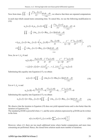
Now, the inverse operator L–1
is an integral operator which is given by
L dt dt dt c t c t c
z times
z z
z
− − −
( ) = … ( ) … + + +…+
∫∫ ∫
1
1
1
2
2
. .
(14)
where c1
, c2
,…, cz
are integral constants.
To solve (10) by means of q-HAM, we choose the initial approximation:
u x t f x f x t f x
t
f x
t
z
z
z
0 0 1 2
2
1
1
2 1
,
! ( )!
( ) = ( )+ ( ) + ( ) +…+ ( )
−
−
−
(15)
Let (x, t)=1, by means of Equations (14) and (15) then Equation (13) becomes
u x t k u x t h
u x
Au x
m m m
t
t t
z
m
z m
, , (
,
,
( ) = ( )+ …
∂ ( )
∂
+ ( )+
−
−
−
∫
∫ ∫
1 0
0 0
1
1
τ
τ
τ B
B u x d d d
m
z times
( , ))
− ( ) …
1
τ τ τ τ (16)](https://image.slidesharecdn.com/06ajms25620-compressed-210322064757/85/Solving-High-order-Non-linear-Partial-Differential-Equations-by-Modified-q-Homotopy-Analysis-Method-3-320.jpg)
![Huseen, et al.: Solving high-order non-linear partial differential equations
AJMS/Apr-Jun-2020/Vol 4/Issue 2 29
THE PROPOSED MQ-HAM
When z≥2, we rewrite Equation (1) as the following system of the first-order differential equations
ut
=u1
u1t
=u2
⋮ (21)
u{z–1}t
=–Au(x, t)–Bu(x, t)
Set the initial approximation
u0
(x, t)=f0
(x),
u10
(x, t)=f1
(x),
⋮ (22)
u{z–1}0
(x, t)=f(z–1) (x)
Using the iteration formulas (18) and (19) as follows
u x t h u x d
t
1 0 0
1
( , ) , ,
= − ( )
( )
∫ τ τ
u x t h u x d
t
1 2
1 0 0
( , ) ,
= − ( )
( )
∫ τ τ (23)
⋮
u z x t h Au x B u x d
t
{ } ( , ) , ( , )
− = ( )+ ( )
( )
∫
1 1
0
0 0
τ τ τ
For m1, km
=n and
um
(x, 0)=0, u1m
(x, 0)=0, u2m
(x, 0)=0,…,u{z–1}m
(x, 0)=0
Substituting in Equation (17), we obtain
u x t n h u x t h u x d
m m
t
m
, , , ,
( ) = +
( ) ( )+ − ( )
( )
− −
∫
1 0 1
1 τ τ
u x t n h u x t h u x d
m m
t
m
1 1 2
1 0 1
, , ,
( ) = +
( ) ( )+ − ( )
( )
− −
∫ τ τ (24)
⋮
u z x t n h u z x t h Au x B u x
m m
t
m m
{ } , { } , , ( ,
− ( ) = +
( ) − ( )+ ( )+ (
− − −
∫
1 1 1
0
1 1
τ τ )
)
( )
) dτ
To illustrate the effectiveness of the proposed mq-HAM, comparison between mq-HAM and the standard
q-HAM is illustrated by the following examples.
ILLUSTRATIVE EXAMPLES[8,9]
We choose the following two cases when z=2 and z=3.
Case 1. z=2
Consider the modified Boussinesq equation
utt
–uxxxx
– (u3
)xx
=0(25)
subject to the initial conditions](https://image.slidesharecdn.com/06ajms25620-compressed-210322064757/85/Solving-High-order-Non-linear-Partial-Differential-Equations-by-Modified-q-Homotopy-Analysis-Method-5-320.jpg)
![Huseen, et al.: Solving high-order non-linear partial differential equations
AJMS/Apr-Jun-2020/Vol 4/Issue 2 30
u x x
, [ ]
0 2
( ) = sech
u x x x
t , [ ]
0 2
( ) = [ ]
sech tanh (26)
The exact solution is
u x t x t
, [ ]
( ) = −
2sech (27)
This problem solved by HAM (q-HAM [n=1]) and nHAM (mq-HAM [n=1]),[7]
so we will solve it by
q-HAM and mq-HAM and compare the results.
IMPLEMENTATION OF Q-HAM
We choose the initial approximation
u0
(x, t)=u(x, 0)+tut
(x, 0)
= [ ]+ [ ]
2 2
sech sech tanh
x t x x
[ ](28)
and the linear operator:
L x t q
x t q
t
[ , ; ]
( , ; )
,
∅( ) =
∂ ∅
∂
2
2
(29)
with the property:
L[c0
+c1t]=0,(30)
where c0
and c1
are real constants.
We define the nonlinear operator by
N x t q
x t q
t
x t q
x x
x t q
∅( )
=
∂ ∅
∂
−
∂ ∅
∂
−
∂
∂
∅( )
, ;
( , ; ) ( , ; )
[ , ; ]
2
2
4
4
2
2
3
(31)
According to the zero-order deformation Equation (2) and the mth-order deformation equation (7) with
R u
u
t
u
x x
u u u
m
m m
i
m
m i j
i
j i
−
− −
=
−
− − = −
( )=
∂
∂
−
∂
∂
−
∂
∂
∑ ∑
1
2
1
2
4
1
4
2
2 0
1
1 0
( j
j ) (32)
The solution of the mth-order deformation equation (7) for m≥1 takes the form
u x t k u x t h R u dt dt c c t
m m m m
, ,
( ) = ( )+ ( ) + +
− −
∫∫
1 1 0 1
(33)
where the coefficients c0
and c1
are determined by the initial conditions:
u x
u x
t
m
m
, ,
,
0 0
0
0
( ) =
∂ ( )
∂
= (34)
Obviously, we obtain
u x t ht x t x t
1
2 8 2 2
1
960 2
135 5 56 15 19 412
, [ ] ( ( ) [ ] ( )
( ) = − − + − +
Sech Cosh C
Cosh Cosh
Cosh Cosh Sinh
[ ] [ ]
[ ] [ ] [ ]
3 15 5
540 5 15 7 215
2
x x
t x x t x
− +
+ − +
6
6120 315 3 1836 3 95 5
108
3 3
t x t x t x t x
Sinh Sinh Sinh Sinh
[ ] [ ] [ ] [ ]
− − − +
t
t x t x
3
5 5 7
Sinh Sinh
[ ] [ ])
+](https://image.slidesharecdn.com/06ajms25620-compressed-210322064757/85/Solving-High-order-Non-linear-Partial-Differential-Equations-by-Modified-q-Homotopy-Analysis-Method-6-320.jpg)
![Huseen, et al.: Solving high-order non-linear partial differential equations
AJMS/Apr-Jun-2020/Vol 4/Issue 2 31
u x t h h n t x t x
2
2 8 2
1
960 2
135 5 56
15 19 4
, ( ) ( ( ) [ ]
(
( ) = − + [ ] − +
− +
Sech Cosh
1
12 3 15 5 540 5 15 7
215
2 2
t x x t x x
t
) [ ] [ ] [ ] [ ]
Cosh Cosh Cosh Cosh
Sin
− + +
− h
h Sinh Sinh Sinh
Sinh
[ ] [ ] [ ] [ ]
[
x t x t x t x
t x
+ − −
−
6120 315 3 1836 3
95 5
3 3
]
] [ ] [ ])
(
+ +
+ − [ ] + [ ]
108 5 5 7
1
160 2
1 2
3
10
t x t x
h ht x x
Sinh Sinh
Sech Cosh +
+ [ ]
( ) − +…
Sinh Cosh
2 1 6 2
3
x x
( [ ]
(34)
um
(x, t), (m=3,4,…) can be calculated similarly. Then, the series solution expression by q-HAM can be
written in the form:
u x t n h U x t n h u x t n h
n
M i
M
i
i
, ; ; , ; ; , ; ;
( ) ( ) = ( )
=
∑
≅ 0
1
(35)
Equation (35) is a family of approximation solutions to the problem (25) in terms of the convergence
parameters h and n. To find the valid region of h, the h curves given by the 3rd
order q-HAM approximation
at different values of x, t, and n are drawn in Figures 1-3. This figure shows the interval of h which the
value of U3
(x, t; n) is constant at certain x, t, and n, We choose the line segment nearly parallel to the
horizontal axis as a valid region of h which provides us with a simple way to adjust and control the
convergence region. Figures 4 and 5 show the comparison between U3
of q-HAM using different values
of n with the solution (27). The absolute errors of the 3rd
order solutions q-HAM approximate using
different values of n are shown in Figures 6 and 7.
IMPLEMENTATION OF MQ-HAM
To solve Equation (25) by mq-HAM, we construct system of differential equations as follows
ut
(x, t)=v(x, t),
v x t
u x t
x x
u x t
t ,
( , )
[ , ]
( ) =
∂
∂
+
∂
∂
( )
4
4
2
2
3
(36)
with initial approximations
u x t x v x t x x
0 0
2 2
, , , [ ]
( ) = [ ] ( ) = [ ]
sech sech tanh (37)
and the auxiliary linear operators
Figure 1: h curve for the (q-HAM; n=1) (HAM) approximation solution U3
(x, t; 1) of problem (25) at different values of x
and t](https://image.slidesharecdn.com/06ajms25620-compressed-210322064757/85/Solving-High-order-Non-linear-Partial-Differential-Equations-by-Modified-q-Homotopy-Analysis-Method-7-320.jpg)


![Huseen, et al.: Solving high-order non-linear partial differential equations
AJMS/Apr-Jun-2020/Vol 4/Issue 2 34
v x t h
u x
x x
u x d
t
1 0
4
0
4
2
2 0
3
,
,
,
( ) = −
∂ ( )
∂
−
∂
∂
( )
( )
∫
τ
τ τ .
Now, form ≥2, we get
u x t n h u x t h v x d
m m
t
m
, , ,
( ) = +
( ) ( )+ − ( )
( )
− −
∫
1 0 1 τ τ (41)
v x t n h v x t h
u x
x x
u
m m
t
m
i
m
m
, ,
( , )
(
( ) = +
( ) ( )+ −
∂
∂
−
∂
∂
−
−
=
−
∫ ∑
1
0
4
1
4
2
2
0
1
τ
−
− −
=
−
∑ ( )
1
0
i
j
i
j i j
x u x u x d
( , ) , ( , ))
τ τ τ τ
And the following results are obtained
u x t ht x x
1 2
, [ ] [ ]
( ) = − Sech Tanh
v x t ht x x x
1
5 4
2 2
, ( [ ] [ ] [ ] )
( ) = −
Sech Sech Tanh
u x t
h t x x
h h n t x x
2
2 2 3
3 2
2 2
2
,
( [ ]) [ ]
( ) [ ] [ ]
( ) =
− +
− +
Cosh Sech
Sech Tanh
v x t
h t x x x
h h n t
2
2 2 3
11 2
2 2
2
,
( [ ]) [ ] [ ]
( ) ( [
( ) =
− +
+ +
Cosh Sech Tanh
Sech x
x x x
] [ ] [ ] )
5 4
2
− Sech Tanh
um
(x, t), (m=3, 4,…) can be calculated similarly. Then, the series solution expression by mq- HAM can
be written in the form:
u x t n h U x t n h u x t n h
n
M i
M
i
i
, ; ; , ; ; , ; ;
( ) ( ) = ( )
=
∑
≅ 0
1
(42)
Equation (42) is a family of approximation solutions to the problem (25) in terms of the convergence
parametershandn.Tofindthevalidregionofh,thehcurvesgivenbythe3rd
ordermq-HAMapproximation
at different values of x, t, and n are drawn in Figures 8-10. This figure shows the interval of h which
the value of U3
(x, t; n) is constant at certain x, t, and n. We choose the line segment nearly parallel to
the horizontal axis as a valid region of h which provides us with a simple way to adjust and control the
convergence region. Figure 11 shows the comparison between U3
of mq-HAM using different values
of n with the solution (27). The absolute errors of the 3th
order solutions mq-HAM approximate using
different values of n are shown in Figure 12. The results obtained by mq-HAM are more accurate than
Figure 8: h curve for the (mq-HAM; n=1) approximation solution U3
(x, t; 1) of problem (25) at different values of x and t](https://image.slidesharecdn.com/06ajms25620-compressed-210322064757/85/Solving-High-order-Non-linear-Partial-Differential-Equations-by-Modified-q-Homotopy-Analysis-Method-10-320.jpg)


![Huseen, et al.: Solving high-order non-linear partial differential equations
AJMS/Apr-Jun-2020/Vol 4/Issue 2 37
This problem solved by HAM (q-HAM (n=1)) and nHAM (mq-HAM (n=1)),[7]
so we will solve it by
q-HAM and mq-HAM and compare the results.
IMPLEMENTATION OF Q-HAM
We choose the initial approximation
u x t
x
t
x
t
x
0 2 4
2
6
1
,
( ) = − − − (46)
Figure 15: The comparison between the U3
(x, t) of q-HAM (n=100), U3
(x, t) of mq-HAM (n=100), U5
(x, t) of mq-HAM
(n=100), and the exact solution of Equation (25) at h=–70 and x=0
Figure 16: The comparison between the U3
(x, t) of q-HAM (n=100), U3
(x, t) of mq-HAM (n=100), U5
(x, t) of mq-HAM
(n=100), and the exact solution of Equation (25) at h=–70 and x=1
Figure 17: The comparison between the absolute error of U3
(x, t) of q-HAM (n=1) and U3
(x, t) of mq-HAM (n=1) of
Equation (25) at h=–1, x=0 and-1≤t≤1](https://image.slidesharecdn.com/06ajms25620-compressed-210322064757/85/Solving-High-order-Non-linear-Partial-Differential-Equations-by-Modified-q-Homotopy-Analysis-Method-13-320.jpg)
![Huseen, et al.: Solving high-order non-linear partial differential equations
AJMS/Apr-Jun-2020/Vol 4/Issue 2 38
and the linear operator:
L x t q
x t q
t
[ , ; ]
( , ; )
∅( ) =
∂ ∅
∂
3
3
(47)
with the property:
L c c t c t
0 1 2
2
0
+ +
= (48)
where c0
, c1
, and c2
are real constants.
Figure 18: The comparison between the absolute error of U3
(x, t) of q-HAM (n=100) and U3
(x, t) of mq-HAM (n=100) of
Equation (25) at h=–70, x=0 and –1≤t≤1
Figure 19: The comparison between the absolute error of U3
(x, t) of mq-HAM (n=1) and U5
(x, t) of mq-HAM (n=1) of
Equation (25) at h=–1, x=1 and –1.5≤t≤1.5
Figure 20: The comparison between the absolute error of U3
(x, t) of mq-HAM (n=100) and U5
(x, t) of mq-HAM (n=100)
of Equation (25) at h=–70, x=1 and –1.5≤t≤1.5](https://image.slidesharecdn.com/06ajms25620-compressed-210322064757/85/Solving-High-order-Non-linear-Partial-Differential-Equations-by-Modified-q-Homotopy-Analysis-Method-14-320.jpg)
![Huseen, et al.: Solving high-order non-linear partial differential equations
AJMS/Apr-Jun-2020/Vol 4/Issue 2 39
Next, we define the nonlinear operator by
N x t q
x t q
t
x t q
x
x x t q x
∅( )
=
∂ ∅
∂
+
∂∅
∂
− ∅( ) + ∅
, ;
( , ; ) ( , ; )
[ , ; ] [
3
3
2
2 6 ,
, ; ]
t q
( ) 4
(49)
According to the zero-order deformation Equation (2) and the mth
-order deformation equation (7) with
R u
u
t
u
x
x u u u
m
m m m
i m i
m
m
i i
−
− − −
− −
−
− −
= =
( )=
∂
∂
+
∂
∂
− +
∑ ∑
1
3
1
3
1 1
1
1
1
0 0
2 6
i
i i j k j k
j
i
k
j
u u u
= =
− −
∑ ∑
0 0
(50)
The solution of the mth
-order deformation equation (7) for m≥1 becomes:
u x t k u x t h R u dt dt dt c c t c t
m m m m
, ,
( ) = ( )+ ( ) + + +
− −
∫∫∫
1 1 0 1 2
2
(51)
where the coefficients c0
, c1
and c2
are determined by the initial conditions:
u x
u x
t
u x
t
m
m m
, ,
,
,
,
0 0
0
0
0
0
2
2
( ) =
∂ ( )
∂
=
∂ ( )
∂
= (52)
We now successively obtain:
u x t
x
ht t t x t x t x
t x
1 24
3 8 7 2 6 4 5 6
2 12
1
2310
14 77 275 660
2310
, (
( ) = + + +
+ + 2
2310 2310 22 57 77 24
14 16 4 8 5 3 10 5
tx x t x x t x x
+ − − + − − +
( ) ( ))
u x t
x
hnt t t x t x t x
t x
2 24
3 8 7 2 6 4 5 6
2 12
1
2310
14 77 275 660
2310
, (
( ) = + + + +
+
+ + − − + − − +
−
2310 2310 22 57 77 24
1
244432
14 16 4 8 5 3 10 5
tx x t x x t x x
( ) ( ))
1
18800
519792 5197920 30603300
1272889
42
2 3 17 16 2 15 4
x
h t t t x t x
( + + +
8
80 10475665200
14 6 5 24
t x t x
+ −…
um
(x, t), (m=3,4,…) can be calculated similarly. Then, the series solution expression by q- HAM can be
written in the form:
u x t n h U x t n h u x t n h
n
M i
M
i
i
, ; ; , ; ; , ; ;
( ) ( ) = ( )
=
∑
≅ 0
1
(53)
Equation(53)isafamilyofapproximationsolutionstotheproblem(43)intermsoftheconvergenceparameters
h and n. To find the valid region of h, the h curves given by the 5th
order q-HAM approximation at different
values of x, t, and n are drawn in Figures 21-23. This figure shows the interval of h which the value of U5
(x, t; n) is constant at certain x, t and n. We choose the line segment nearly parallel to the horizontal axis as a
valid region of h which provides us with a simple way to adjust and control the convergence region. Figure 24
shows the comparison between U5
of q-HAM using different values of n with the solution 45. The absolute
errors of the 5th
order solutions q-HAM approximate using different values of n are shown in Figure 25.
IMPLEMENTATION OF MQ-HAM
To solve Equation (43) by mq-HAM, we construct system of differential equations as follows
ut
(x, t)=v(x, t),
vt
(x, t)=w(x, t)(54)
With initial approximations
u x t
x
v x t
x
w x t
x
0 2 0 4 0 6
1 1 2
, , , , ,
( ) = − ( ) = − ( ) = − (55)](https://image.slidesharecdn.com/06ajms25620-compressed-210322064757/85/Solving-High-order-Non-linear-Partial-Differential-Equations-by-Modified-q-Homotopy-Analysis-Method-15-320.jpg)


Solving High-order Non-linear Partial Differential Equations by Modified q-Homotopy Analysis Method
- 1. www.ajms.com 25 ISSN 2581-3463 RESEARCH ARTICLE Solving High-order Non-linear Partial Differential Equations by Modified q-Homotopy Analysis Method Shaheed N. Huseen1 , Magdy A. El-Tawil2 , Said R. Grace2 , Gamal A. F. Ismail3 1 Department of Mathematics, Faculty of Computer Science and Mathematics, University of Thi-Qar, Iraq, 2 Department of Engineering Mathematics, Faculty of Engineering, Cairo University, Giza, Egypt, 3 Department of Mathematics, Women’s Faculty, Ain Shams University, Egypt Received: 25-04-2020; Revised: 25-05-2020; Accepted: 10-06-2020 ABSTRACT In this paper, modified q-homotopy analysis method (mq-HAM) is proposed for solving high-order non-linear partial differential equations. This method improves the convergence of the series solution and overcomes the computing difficulty encountered in the q-HAM, so it is more accurate than nHAM which proposed in Hassan and El-Tawil, Saberi-Nik and Golchaman. The second- and third-order cases are solved as illustrative examples of the proposed method. Key words: Non-linear partial differential equations, q-homotopy analysis method, modified q-homotopy analysis method INTRODUCTION Most phenomena in our world are essentially non-linear and are described by non-linear equations. It is still difficult to obtain accurate solutions of non-linear problems and often more difficult to get an analytic approximation than a numerical one of a given non-linear problem. In 1992, Liao[1] employed the basic ideas of the homotopy in topology to propose a general analytic method for non- linear problems, namely, homotopy analysis method (HAM). In recent years, this method has been successfully employed to solve many types of non-linear problems in science and engineering.[2-11] All of these successful applications verified the validity, effectiveness, and flexibility of the HAM. The HAM contains a certain auxiliary parameter h which provides us with a simple way to adjust and control the convergence region and rate of convergence of the series solution. Moreover, by means of the so-called h-curve, it is easy to determine the valid regions of h to gain a convergent series solution. Hassan and El-Tawil[7] presented a new technique of using HAM for solving high-order non-linear initial value problems (nHAM) by transform the nth-order non-linear differential equation to a system of n first-order equations. El-Tawil and Huseen[12] established a method, namely, q-HAM which is a more general method of HAM. The q-HAM contains an auxiliary parameter n as well as h such that the case of n=1 (q-HAM; n=1) the standard HAM can be reached. The q-HAM has been successfully applied to numerous problems in science and engineering.[12-22] Huseen and Grace[23] presented modifications of q-HAM (mq-HAM). They tested the scheme on two second-order non- linear exactly solvable differential equations. The aim of this paper is to apply the mq-HAM to obtain the approximate solutions of high-order non-linear problems by transform the nth-order non-linear differential equation to a system of n first-order equations. We note that the case of n=1 in mq-HAM (mq-HAM; n=1), the nHAM[7] can be reached. Address for correspondence: Shaheed N. Huseen, E-mail: [email protected]
- 2. Huseen, et al.: Solving high-order non-linear partial differential equations AJMS/Apr-Jun-2020/Vol 4/Issue 2 26 ANALYSIS OF THE Q-HAM Consider the following non-linear partial differential equation: N[u(x, t)]=0(1) Where, N is a non-linear operator, (x, t) denotes independent variables, and u(x, t) is an unknown function. Let us construct the so-called zero-order deformation equation: (1–nq)L[∅(x, t; q)–u0 (x, t)]=qhH(x, t)N[∅(x, t; q)](2) where n≥1, q∈[0, 1 n ] denotes the so-called embedded parameter, L is an auxiliary linear operator with the property L[f]=0 when f=0, h≠0 is an auxiliary parameter, H(x, t) denotes a non-zero auxiliary function. It is obvious that when q=0 and q= 1 n Equation (2) becomes ∅( ) = ( ) ∅ = x t u x t and x t n u x t , ; , , ; ( , ) 0 1 0 (3) respectively. Thus, as q increases from 0 to 1 n , the solution ∅(x, t; q) varies from the initial guess u0 (x, t) to the solution (x, t). We may choose u0 (x, t), L, h, H (x, t) and assume that all of them can be properly chosen so that the solution ∅(x, t; q) of Equation (2) exists for q∈[0, 1 n ]. Now, by expanding ∅(x, t; q) in Taylor series, we have ∅( ) = ( )+ = +∞ ∑ x t q u x t u x t q m m m , ; , ( , ) 0 1 (4) where u x t m x t q q m m m q , ! ( , ; ) | ( ) = ∂ ∅ ∂ = 1 0 (5) Next, we assume that h, H (x, t), u0 (x, t), L are properly chosen such that the series (4) converges at q= 1 n and: u x t x t n u x t u x t n m m m , , ; , , ( ) = ∅ = ( )+ ( ) = +∞ ∑ 1 1 0 1 (6) We let u x t u x t u x t u x t u x t r r , , , , , , , , , ( ) = ( ) ( ) ( ) … ( ) { } 0 1 2 Differentiating equation (2) m times with respect to q and then setting q=0 and dividing the resulting equation by m! we have the so-called mth order deformation equation L u x t k u x t hH x t R u x t m m m m m , , , ( , ) ( )− ( ) = ( ) ( ) − − 1 1 (7) where, R u x t m N x t q f x t q m m m m q ( , ) ! ( , ; , ) | − − − = ( ) = − ( ) ∂ ∅( ) − ( ) ∂ 1 1 1 0 1 1 (8)
- 3. Huseen, et al.: Solving high-order non-linear partial differential equations AJMS/Apr-Jun-2020/Vol 4/Issue 2 27 and k m n otherwise m = ≤ 0 1 (9) It should be emphasized that um (x, t) for m≥1 is governed by the linear Equation (7) with linear boundary conditions that come from the original problem. Due to the existence of the factor 1 n m , more chances for convergence may occur or even much faster convergence can be obtained better than the standard HAM. It should be noted that the case of n=1 in Equation (2), standard HAM can be reached. The q-HAM can be reformatted as follows: We rewrite the nonlinear partial differential equation (1) in the form Lu x t Au x t Bu x t , , , ( )+ ( )+ ( ) = 0 u x f x , , 0 0 ( ) = ( ) ∂ ∂ = ( ) = u x t t f x t ( , ) | , 0 1 (10) ∂ ∂ = − − = − ( ) ( ) ( ) ( ) ( , ) | ( ), z z t z u x t f x 1 1 0 1 Where, L t z z = ∂ ∂ ( ) , z=1,2,… is the highest partial derivative with respect to t, A is a linear term, and B is non-linear term. The so-called zero-order deformation Equation (2) becomes: 1 0 − ( ) ∅( )− = ( ) ( )+ ( )+ nq L x t q u x t qhH x t Lu x t Au x t Bu x t , ; ( , ) , ( , , , ( ( ))(11) we have the mth order deformation equation L u x t k u x t hH x t Lu x t Au x t B u m m m m m , , , ( , , ( ( )− ( ) = ( ) ( )+ ( )+ − − − 1 1 1 m m x t − ( ) 1 , )) (12) and hence u x t k u x t hL H x t Lu x t Au x t B u m m m m m m , , [ , ( , , ( ( ) = ( )+ ( ) ( )+ ( )+ − − − − 1 1 1 1 − − ( ) 1 x t , ))](13) Now, the inverse operator L–1 is an integral operator which is given by L dt dt dt c t c t c z times z z z − − − ( ) = … ( ) … + + +…+ ∫∫ ∫ 1 1 1 2 2 . . (14) where c1 , c2 ,…, cz are integral constants. To solve (10) by means of q-HAM, we choose the initial approximation: u x t f x f x t f x t f x t z z z 0 0 1 2 2 1 1 2 1 , ! ( )! ( ) = ( )+ ( ) + ( ) +…+ ( ) − − − (15) Let (x, t)=1, by means of Equations (14) and (15) then Equation (13) becomes u x t k u x t h u x Au x m m m t t t z m z m , , ( , , ( ) = ( )+ … ∂ ( ) ∂ + ( )+ − − − ∫ ∫ ∫ 1 0 0 0 1 1 τ τ τ B B u x d d d m z times ( , )) − ( ) … 1 τ τ τ τ (16)
- 4. Huseen, et al.: Solving high-order non-linear partial differential equations AJMS/Apr-Jun-2020/Vol 4/Issue 2 28 Now from times 0 0 0 1 t t t z m z z times u x d d d ∫ ∫ ∫ … ∂ ( ) ∂ … − ( ,τ τ τ τ τ , we observe that there are repeated computations in each step which caused more consuming time. To cancel this, we use the following modification to (16): u x t k u x t h u x d d d m m m t t t z m z z times , , , ( ) = ( )+ … ∂ ( ) ∂ … − − ∫ ∫ ∫ 1 0 0 0 1 τ τ τ τ τ + … ( )+ ( ) … ∫ ∫ ∫ − − h Au x B u x d d d t t t m m z times 0 0 0 1 1 ( , ( , )) τ τ τ τ τ = ( )+ ( )− ( )+ ∂ ( ) ∂ +…+ − − − − − − k u x t hu x t h u x t u x t t z m m m m m z 1 1 1 1 1 0 0 1 , , , , ( ( ) ∂ ( ) ∂ + + … ( )+ − − − − ∫ ∫ ∫ ! , ( , ( z m z t t t m u x t h Au x B u 1 1 1 0 0 0 1 0 τ m m ztimes x d d d − ( ) … 1 , )) τ τ τ τ (17) Now, for m=1, km =0 and u x t u x t t u x t t z u x z z 0 0 2 2 0 2 1 1 0 0 0 2 0 1 0 , , ! , ! , ( )+ ∂ ( ) ∂ + ∂ ( ) ∂ …+ − ( ) ∂ ( − − ) ) ∂ = ( )+ ( ) + ( ) +…+ ( ) − = ( ) − − − t f x f x t f x t f x t z u x t z z z 1 0 1 2 2 1 1 0 2 1 ! ( )! , Substituting this equality into Equation (17), we obtain u x t h Au x B u x d d d t t t z times 1 0 0 0 0 0 , ( , ( , )) ( ) = … ( )+ ( ) … ∫ ∫ ∫ τ τ τ τ τ (18) For m1, km =n and u x u x t u x t u x t m m m z m z , , , , , , , , 0 0 0 0 0 0 0 0 2 2 1 1 ( ) = ∂ ( ) ∂ = ∂ ( ) ∂ = … ∂ ( ) ∂ = − − Substituting this equality into Equation (17), we obtain u x t n h u x t h Au x B u x m m t t t m m , , ( , ( , ( ) = + ( ) ( )+ … ( )+ ( ) − − − ∫ ∫ ∫ 1 0 0 0 1 1 τ τ ) ))d d d z times τ τ τ … (19) We observe that the iteration in Equation (19) does not yield repeated terms and is also better than the iteration in Equation (16). The standard q-HAM is powerful when z=1, and the series solution expression by q-HAM can be written in the form ( ) ( ) ( ) 0 1 , ; ; , ; ; , ; ; = ≅ = ∑ i M M i i u x t n h U x t n h u x t n h n (20) However, when z≥2, there are too much additional terms where harder computations and more time consuming are performed. Hence, the closed form solution needs more number of iterations.
- 5. Huseen, et al.: Solving high-order non-linear partial differential equations AJMS/Apr-Jun-2020/Vol 4/Issue 2 29 THE PROPOSED MQ-HAM When z≥2, we rewrite Equation (1) as the following system of the first-order differential equations ut =u1 u1t =u2 ⋮ (21) u{z–1}t =–Au(x, t)–Bu(x, t) Set the initial approximation u0 (x, t)=f0 (x), u10 (x, t)=f1 (x), ⋮ (22) u{z–1}0 (x, t)=f(z–1) (x) Using the iteration formulas (18) and (19) as follows u x t h u x d t 1 0 0 1 ( , ) , , = − ( ) ( ) ∫ τ τ u x t h u x d t 1 2 1 0 0 ( , ) , = − ( ) ( ) ∫ τ τ (23) ⋮ u z x t h Au x B u x d t { } ( , ) , ( , ) − = ( )+ ( ) ( ) ∫ 1 1 0 0 0 τ τ τ For m1, km =n and um (x, 0)=0, u1m (x, 0)=0, u2m (x, 0)=0,…,u{z–1}m (x, 0)=0 Substituting in Equation (17), we obtain u x t n h u x t h u x d m m t m , , , , ( ) = + ( ) ( )+ − ( ) ( ) − − ∫ 1 0 1 1 τ τ u x t n h u x t h u x d m m t m 1 1 2 1 0 1 , , , ( ) = + ( ) ( )+ − ( ) ( ) − − ∫ τ τ (24) ⋮ u z x t n h u z x t h Au x B u x m m t m m { } , { } , , ( , − ( ) = + ( ) − ( )+ ( )+ ( − − − ∫ 1 1 1 0 1 1 τ τ ) ) ( ) ) dτ To illustrate the effectiveness of the proposed mq-HAM, comparison between mq-HAM and the standard q-HAM is illustrated by the following examples. ILLUSTRATIVE EXAMPLES[8,9] We choose the following two cases when z=2 and z=3. Case 1. z=2 Consider the modified Boussinesq equation utt –uxxxx – (u3 )xx =0(25) subject to the initial conditions
- 6. Huseen, et al.: Solving high-order non-linear partial differential equations AJMS/Apr-Jun-2020/Vol 4/Issue 2 30 u x x , [ ] 0 2 ( ) = sech u x x x t , [ ] 0 2 ( ) = [ ] sech tanh (26) The exact solution is u x t x t , [ ] ( ) = − 2sech (27) This problem solved by HAM (q-HAM [n=1]) and nHAM (mq-HAM [n=1]),[7] so we will solve it by q-HAM and mq-HAM and compare the results. IMPLEMENTATION OF Q-HAM We choose the initial approximation u0 (x, t)=u(x, 0)+tut (x, 0) = [ ]+ [ ] 2 2 sech sech tanh x t x x [ ](28) and the linear operator: L x t q x t q t [ , ; ] ( , ; ) , ∅( ) = ∂ ∅ ∂ 2 2 (29) with the property: L[c0 +c1t]=0,(30) where c0 and c1 are real constants. We define the nonlinear operator by N x t q x t q t x t q x x x t q ∅( ) = ∂ ∅ ∂ − ∂ ∅ ∂ − ∂ ∂ ∅( ) , ; ( , ; ) ( , ; ) [ , ; ] 2 2 4 4 2 2 3 (31) According to the zero-order deformation Equation (2) and the mth-order deformation equation (7) with R u u t u x x u u u m m m i m m i j i j i − − − = − − − = − ( )= ∂ ∂ − ∂ ∂ − ∂ ∂ ∑ ∑ 1 2 1 2 4 1 4 2 2 0 1 1 0 ( j j ) (32) The solution of the mth-order deformation equation (7) for m≥1 takes the form u x t k u x t h R u dt dt c c t m m m m , , ( ) = ( )+ ( ) + + − − ∫∫ 1 1 0 1 (33) where the coefficients c0 and c1 are determined by the initial conditions: u x u x t m m , , , 0 0 0 0 ( ) = ∂ ( ) ∂ = (34) Obviously, we obtain u x t ht x t x t 1 2 8 2 2 1 960 2 135 5 56 15 19 412 , [ ] ( ( ) [ ] ( ) ( ) = − − + − + Sech Cosh C Cosh Cosh Cosh Cosh Sinh [ ] [ ] [ ] [ ] [ ] 3 15 5 540 5 15 7 215 2 x x t x x t x − + + − + 6 6120 315 3 1836 3 95 5 108 3 3 t x t x t x t x Sinh Sinh Sinh Sinh [ ] [ ] [ ] [ ] − − − + t t x t x 3 5 5 7 Sinh Sinh [ ] [ ]) +
- 7. Huseen, et al.: Solving high-order non-linear partial differential equations AJMS/Apr-Jun-2020/Vol 4/Issue 2 31 u x t h h n t x t x 2 2 8 2 1 960 2 135 5 56 15 19 4 , ( ) ( ( ) [ ] ( ( ) = − + [ ] − + − + Sech Cosh 1 12 3 15 5 540 5 15 7 215 2 2 t x x t x x t ) [ ] [ ] [ ] [ ] Cosh Cosh Cosh Cosh Sin − + + − h h Sinh Sinh Sinh Sinh [ ] [ ] [ ] [ ] [ x t x t x t x t x + − − − 6120 315 3 1836 3 95 5 3 3 ] ] [ ] [ ]) ( + + + − [ ] + [ ] 108 5 5 7 1 160 2 1 2 3 10 t x t x h ht x x Sinh Sinh Sech Cosh + + [ ] ( ) − +… Sinh Cosh 2 1 6 2 3 x x ( [ ] (34) um (x, t), (m=3,4,…) can be calculated similarly. Then, the series solution expression by q-HAM can be written in the form: u x t n h U x t n h u x t n h n M i M i i , ; ; , ; ; , ; ; ( ) ( ) = ( ) = ∑ ≅ 0 1 (35) Equation (35) is a family of approximation solutions to the problem (25) in terms of the convergence parameters h and n. To find the valid region of h, the h curves given by the 3rd order q-HAM approximation at different values of x, t, and n are drawn in Figures 1-3. This figure shows the interval of h which the value of U3 (x, t; n) is constant at certain x, t, and n, We choose the line segment nearly parallel to the horizontal axis as a valid region of h which provides us with a simple way to adjust and control the convergence region. Figures 4 and 5 show the comparison between U3 of q-HAM using different values of n with the solution (27). The absolute errors of the 3rd order solutions q-HAM approximate using different values of n are shown in Figures 6 and 7. IMPLEMENTATION OF MQ-HAM To solve Equation (25) by mq-HAM, we construct system of differential equations as follows ut (x, t)=v(x, t), v x t u x t x x u x t t , ( , ) [ , ] ( ) = ∂ ∂ + ∂ ∂ ( ) 4 4 2 2 3 (36) with initial approximations u x t x v x t x x 0 0 2 2 , , , [ ] ( ) = [ ] ( ) = [ ] sech sech tanh (37) and the auxiliary linear operators Figure 1: h curve for the (q-HAM; n=1) (HAM) approximation solution U3 (x, t; 1) of problem (25) at different values of x and t
- 8. Huseen, et al.: Solving high-order non-linear partial differential equations AJMS/Apr-Jun-2020/Vol 4/Issue 2 32 Lu x t u x t t Lv x t v x t t , ( , ) , , ( , ) ( ) = ∂ ∂ ( ) = ∂ ∂ (38) and Au x t u x t x m m − − ( ) = − ∂ ∂ 1 4 1 4 , ( , ) Figure 2: h curve for the (q-HAM; n=50) approximation solution U3 (x, t; 50) of problem (25) at different values of x and t Figure 3: h curve for the (q-HAM; n=100) approximation solution U3 (x, t; 100) of problem (25) at different values of x and t Figure 4: Comparison between U3 of q-HAM (n=1, 2, 5, 10, 20, 50, 100) with exact solution of Equation (25) at x=0 with h=–1, h=–1.8, h=–4.5, (h=–8, h=–15.2, h=–37, h=–70), respectively
- 9. Huseen, et al.: Solving high-order non-linear partial differential equations AJMS/Apr-Jun-2020/Vol 4/Issue 2 33 Bu x t x u x t u x t u x t m i m m i j i j i j − = − − − = − ( ) = − ∂ ∂ ( ) ∑ ∑ 1 2 2 0 1 1 0 , ( ( , ) , ( , )) ) (39) From Equations (23) and (24) we obtain: u x t h v x d t 1 0 0 , , ( ) = − ( ) ( ) ∫ τ τ (40) Figure 5: Comparison between U3 of q-HAM (n=1, 2, 5, 10, 20, 50, 100) with exact solution of Equation (25) at x=1 with (h=–1, h=–1.8, h=–4.5, h=–8, h=–15.2, h=–37, h=–70), respectively Figure 6: The absolute error of U3 of q-HAM (n=1, 2, 5, 10, 20, 50, 100) for problem (25) at x=0 using (h=–1, h=–1.8, h=–4.5, h=–8, h=–15.2, h=–37, h=–70), respectively Figure 7: The absolute error of U3 of q-HAM (n=1, 2, 5, 10, 20, 50, 100) for problem (25) at x=1 using (h=–1, h=–1.8, h=–4.5, h=–8, h=–15.2, h=–37, h=–70), respectively
- 10. Huseen, et al.: Solving high-order non-linear partial differential equations AJMS/Apr-Jun-2020/Vol 4/Issue 2 34 v x t h u x x x u x d t 1 0 4 0 4 2 2 0 3 , , , ( ) = − ∂ ( ) ∂ − ∂ ∂ ( ) ( ) ∫ τ τ τ . Now, form ≥2, we get u x t n h u x t h v x d m m t m , , , ( ) = + ( ) ( )+ − ( ) ( ) − − ∫ 1 0 1 τ τ (41) v x t n h v x t h u x x x u m m t m i m m , , ( , ) ( ( ) = + ( ) ( )+ − ∂ ∂ − ∂ ∂ − − = − ∫ ∑ 1 0 4 1 4 2 2 0 1 τ − − − = − ∑ ( ) 1 0 i j i j i j x u x u x d ( , ) , ( , )) τ τ τ τ And the following results are obtained u x t ht x x 1 2 , [ ] [ ] ( ) = − Sech Tanh v x t ht x x x 1 5 4 2 2 , ( [ ] [ ] [ ] ) ( ) = − Sech Sech Tanh u x t h t x x h h n t x x 2 2 2 3 3 2 2 2 2 , ( [ ]) [ ] ( ) [ ] [ ] ( ) = − + − + Cosh Sech Sech Tanh v x t h t x x x h h n t 2 2 2 3 11 2 2 2 2 , ( [ ]) [ ] [ ] ( ) ( [ ( ) = − + + + Cosh Sech Tanh Sech x x x x ] [ ] [ ] ) 5 4 2 − Sech Tanh um (x, t), (m=3, 4,…) can be calculated similarly. Then, the series solution expression by mq- HAM can be written in the form: u x t n h U x t n h u x t n h n M i M i i , ; ; , ; ; , ; ; ( ) ( ) = ( ) = ∑ ≅ 0 1 (42) Equation (42) is a family of approximation solutions to the problem (25) in terms of the convergence parametershandn.Tofindthevalidregionofh,thehcurvesgivenbythe3rd ordermq-HAMapproximation at different values of x, t, and n are drawn in Figures 8-10. This figure shows the interval of h which the value of U3 (x, t; n) is constant at certain x, t, and n. We choose the line segment nearly parallel to the horizontal axis as a valid region of h which provides us with a simple way to adjust and control the convergence region. Figure 11 shows the comparison between U3 of mq-HAM using different values of n with the solution (27). The absolute errors of the 3th order solutions mq-HAM approximate using different values of n are shown in Figure 12. The results obtained by mq-HAM are more accurate than Figure 8: h curve for the (mq-HAM; n=1) approximation solution U3 (x, t; 1) of problem (25) at different values of x and t
- 11. Huseen, et al.: Solving high-order non-linear partial differential equations AJMS/Apr-Jun-2020/Vol 4/Issue 2 35 q-HAM at different values of x and n, so the results indicate that the speed of convergence for mq-HAM with n1 is faster in comparison with n=1 (nHAM). The results show that the convergence region of series solutions obtained by mq-HAM is increasing as q is decreased, as shown in Figures 11 and 12. By increasing the number of iterations by mq-HAM, the series solution becomes more accurate, more efficient and the interval of t (convergent region) increases, as shown in Figures 13-20. Case 2. z=3 Consider the non-linear initial value problem: u x t u x t x u x t u x t ttt x , , , , ( )+ ( )− ( ) ( ) + ( ) ( ) = 2 6 0 2 4 (43) Figure 9: h curve for the (mq-HAM; n=50) approximation solution U3 (x, t; 50) of problem (25) at different values of x and t Figure 10: h curve for the (mq-HAM; n=100) approximation solution U3 (x, t; 100) of problem (25) at different values of x and t Figure 11: Comparison between U3 (x, t) of mq-HAM (n=1, 2, 5, 10, 20, 50, 100) with exact solution of Equation (25) at x=0 with (h=–1, h=–1.8, h=–4.5, h=–8, h=–15.2, h=–37, h=–70), respectively
- 12. Huseen, et al.: Solving high-order non-linear partial differential equations AJMS/Apr-Jun-2020/Vol 4/Issue 2 36 Subject to the initial conditions u x x u x x u x x t tt , , , , , 0 1 0 1 0 2 2 4 6 ( ) = − ( ) = − ( ) = − (44) The exact solution is u x t x t , ( ) = − + 1 2 (45) Figure 12: The absolute error of U3 of mq-HAM (n=1, 2, 5, 10, 20, 50, 100) for problem (25) at x=0 using (h=–1, h=–1.8, h=–4.5, h=–8, h=–15.2, h=–37, h=–70), respectively Figure 13: The comparison between the U3 (x, t) of q-HAM (n=1), U3 (x, t) of mq-HAM (n=1), U5 (x, t) of mq-HAM (n=1), and the exact solution of Equation (25) at h=–1 and x=0 Figure 14: The comparison between the U3 (x, t) of q-HAM (n=1), U3 (x, t) of mq-HAM (n=1), U5 (x, t) of mq-HAM (n=1), and the exact solution of Equation (25) at h=–1 and x=1
- 13. Huseen, et al.: Solving high-order non-linear partial differential equations AJMS/Apr-Jun-2020/Vol 4/Issue 2 37 This problem solved by HAM (q-HAM (n=1)) and nHAM (mq-HAM (n=1)),[7] so we will solve it by q-HAM and mq-HAM and compare the results. IMPLEMENTATION OF Q-HAM We choose the initial approximation u x t x t x t x 0 2 4 2 6 1 , ( ) = − − − (46) Figure 15: The comparison between the U3 (x, t) of q-HAM (n=100), U3 (x, t) of mq-HAM (n=100), U5 (x, t) of mq-HAM (n=100), and the exact solution of Equation (25) at h=–70 and x=0 Figure 16: The comparison between the U3 (x, t) of q-HAM (n=100), U3 (x, t) of mq-HAM (n=100), U5 (x, t) of mq-HAM (n=100), and the exact solution of Equation (25) at h=–70 and x=1 Figure 17: The comparison between the absolute error of U3 (x, t) of q-HAM (n=1) and U3 (x, t) of mq-HAM (n=1) of Equation (25) at h=–1, x=0 and-1≤t≤1
- 14. Huseen, et al.: Solving high-order non-linear partial differential equations AJMS/Apr-Jun-2020/Vol 4/Issue 2 38 and the linear operator: L x t q x t q t [ , ; ] ( , ; ) ∅( ) = ∂ ∅ ∂ 3 3 (47) with the property: L c c t c t 0 1 2 2 0 + + = (48) where c0 , c1 , and c2 are real constants. Figure 18: The comparison between the absolute error of U3 (x, t) of q-HAM (n=100) and U3 (x, t) of mq-HAM (n=100) of Equation (25) at h=–70, x=0 and –1≤t≤1 Figure 19: The comparison between the absolute error of U3 (x, t) of mq-HAM (n=1) and U5 (x, t) of mq-HAM (n=1) of Equation (25) at h=–1, x=1 and –1.5≤t≤1.5 Figure 20: The comparison between the absolute error of U3 (x, t) of mq-HAM (n=100) and U5 (x, t) of mq-HAM (n=100) of Equation (25) at h=–70, x=1 and –1.5≤t≤1.5
- 15. Huseen, et al.: Solving high-order non-linear partial differential equations AJMS/Apr-Jun-2020/Vol 4/Issue 2 39 Next, we define the nonlinear operator by N x t q x t q t x t q x x x t q x ∅( ) = ∂ ∅ ∂ + ∂∅ ∂ − ∅( ) + ∅ , ; ( , ; ) ( , ; ) [ , ; ] [ 3 3 2 2 6 , , ; ] t q ( ) 4 (49) According to the zero-order deformation Equation (2) and the mth -order deformation equation (7) with R u u t u x x u u u m m m m i m i m m i i − − − − − − − − − = = ( )= ∂ ∂ + ∂ ∂ − + ∑ ∑ 1 3 1 3 1 1 1 1 1 0 0 2 6 i i i j k j k j i k j u u u = = − − ∑ ∑ 0 0 (50) The solution of the mth -order deformation equation (7) for m≥1 becomes: u x t k u x t h R u dt dt dt c c t c t m m m m , , ( ) = ( )+ ( ) + + + − − ∫∫∫ 1 1 0 1 2 2 (51) where the coefficients c0 , c1 and c2 are determined by the initial conditions: u x u x t u x t m m m , , , , , 0 0 0 0 0 0 2 2 ( ) = ∂ ( ) ∂ = ∂ ( ) ∂ = (52) We now successively obtain: u x t x ht t t x t x t x t x 1 24 3 8 7 2 6 4 5 6 2 12 1 2310 14 77 275 660 2310 , ( ( ) = + + + + + 2 2310 2310 22 57 77 24 14 16 4 8 5 3 10 5 tx x t x x t x x + − − + − − + ( ) ( )) u x t x hnt t t x t x t x t x 2 24 3 8 7 2 6 4 5 6 2 12 1 2310 14 77 275 660 2310 , ( ( ) = + + + + + + + − − + − − + − 2310 2310 22 57 77 24 1 244432 14 16 4 8 5 3 10 5 tx x t x x t x x ( ) ( )) 1 18800 519792 5197920 30603300 1272889 42 2 3 17 16 2 15 4 x h t t t x t x ( + + + 8 80 10475665200 14 6 5 24 t x t x + −… um (x, t), (m=3,4,…) can be calculated similarly. Then, the series solution expression by q- HAM can be written in the form: u x t n h U x t n h u x t n h n M i M i i , ; ; , ; ; , ; ; ( ) ( ) = ( ) = ∑ ≅ 0 1 (53) Equation(53)isafamilyofapproximationsolutionstotheproblem(43)intermsoftheconvergenceparameters h and n. To find the valid region of h, the h curves given by the 5th order q-HAM approximation at different values of x, t, and n are drawn in Figures 21-23. This figure shows the interval of h which the value of U5 (x, t; n) is constant at certain x, t and n. We choose the line segment nearly parallel to the horizontal axis as a valid region of h which provides us with a simple way to adjust and control the convergence region. Figure 24 shows the comparison between U5 of q-HAM using different values of n with the solution 45. The absolute errors of the 5th order solutions q-HAM approximate using different values of n are shown in Figure 25. IMPLEMENTATION OF MQ-HAM To solve Equation (43) by mq-HAM, we construct system of differential equations as follows ut (x, t)=v(x, t), vt (x, t)=w(x, t)(54) With initial approximations u x t x v x t x w x t x 0 2 0 4 0 6 1 1 2 , , , , , ( ) = − ( ) = − ( ) = − (55)
- 16. Huseen, et al.: Solving high-order non-linear partial differential equations AJMS/Apr-Jun-2020/Vol 4/Issue 2 40 And the auxiliary linear operators Lu x t u x t t Lv x t v x t t Lw x t w x t t , ( , ) , , ( , ) , , ( , ) ( ) = ∂ ∂ ( ) = ∂ ∂ ( ) = ∂ ∂ (56) And Au x t u x t x m m − − ( ) = ∂ ∂ 1 1 , ( , ) Bu x t x u u u u m i m i m i i m m i j i i j k j − = − − − = − − − = − = ( ) = − + ∑ ∑ ∑ 1 0 1 1 0 1 1 0 0 2 6 , ∑ ∑ − u u k j k (57) Figure 21: h curve for the (q-HAM; n=1) (HAM) approximation solution U5 (x, t; 1) of problem (43) at different values of x and t Figure 22: h curve for the (q-HAM; n=20) approximation solution U5 (x, t; 20) of problem (43) at different values of x and t Figure 23: h curve for the (q-HAM; n=100) approximation solution U5 (x, t; 100) of problem (43) at different values of x and t
- 17. Huseen, et al.: Solving high-order non-linear partial differential equations AJMS/Apr-Jun-2020/Vol 4/Issue 2 41 From Equations (23) and (24) we obtain u x t h v x d t 1 0 0 , , ( ) = − ( ) ( ) ∫ τ τ v x t h w x d t 1 0 0 , , ( ) = − ( ) ( ) ∫ τ τ (58) w x t h u x x x u x u x d t 1 0 0 0 2 0 4 2 6 , , , , ( ) = ∂ ( ) ∂ − ( ) ( ) + ( ) ( ) ∫ τ τ τ τ For m≥2, u x t n h u x t h v x d m m t m , , , ( ) = + ( ) ( )+ − ( ) ( ) − − ∫ 1 0 1 τ τ v x t n h v x t h w x d m m t m , , , ( ) = + ( ) ( )+ − ( ) ( ) − − ∫ 1 0 1 τ τ (59) w x t n h w x t h u x t x x u u m m t m i m i m i , , ( , ) ( ) = + ( ) ( )+ ∂ ∂ − + − − = − − − ∫ ∑ 1 0 1 0 1 1 2 6 6 0 1 1 0 0 i m m i j i i j k j k j k u u u u d = − − − = − = − ∑ ∑ ∑ τ The following results are obtained Figure 24: Comparison between U5 of q-HAM (n=1, 2, 5, 10, 20, 50, 100) with exact solution of Equation (43) at x=4 with (h=–1, h=–1.97, h=–4.83, h=–8.45, h=–18.3, h=–44.75, h=–86), respectively Figure 25: The absolute error of U5 of q-HAM (n=1, 2, 5, 10, 20, 50, 100) for problem (43) at x=4 using h=–1, h=–1.97, h=–4.83, h=–8.45, h=–18.3, h=–44.75, h=–86), respectively
- 18. Huseen, et al.: Solving high-order non-linear partial differential equations AJMS/Apr-Jun-2020/Vol 4/Issue 2 42 u x t ht x 1 4 , ( ) = u x t h t x h h n t x 2 2 2 6 4 , ( ) ( ) = − + + u x t h h t x h t x hnt x h n h t x h h n t x 3 2 3 8 2 2 6 2 6 2 2 6 4 , ( ) ( )( ( ) ) ( ) = − − + + − + + um (x, t), (m=4, 5,…) can be calculated similarly. Then, the series solution expression by mq-HAM can be written in the form: u x t n h U x t n h u x t n h n M i M i i , ; ; , ; ; , ; ; ( ) ( ) = ( ) = ∑ ≅ 0 1 (60) Equation (60) is a family of approximation solutions to the problem (43) in terms of the convergence parametershandn.Tofindthevalidregionofh,thehcurvesgivenbythe5th ordermq-HAMapproximation at different values of x, t, and n are drawn in Figures 26-28. This figure shows the interval of h which the value of U5 (x, t; n) is constant at certain x, t, and n. We choose the line segment nearly parallel to the horizontal axis as a valid region of h which provides us with a simple way to adjust and control the convergence region. Figure 29 shows the comparison between U5 of mq-HAM using different values of n with the solution (45). The absolute errors of the 5th order solutions mq-HAM approximate using different values of n are shown in Figure 30. The results obtained by mq-HAM are more accurate than q-HAM at different values of x and n, so the results indicate that the speed of convergence for mq-HAM with n1 is faster in comparison with n=1. (nHAM). The results show that the convergence region of series solutions obtained by mq-HAM is increasing as q is decreased, as shown in Figures 29-36. Figure 26: h curve for the (mq-HAM; n=1) approximation solution U5 (x, t; 1) of problem (43) at different values of x and t Figure 27: h curve for the (mq-HAM; n=20) approximation solution U5 (x, t; 20) of problem (43) at different values of x and t
- 19. Huseen, et al.: Solving high-order non-linear partial differential equations AJMS/Apr-Jun-2020/Vol 4/Issue 2 43 By increasing the number of iterations by mq-HAM, the series solution becomes more accurate, more efficient and the interval of t (convergent region) increases, as shown in Figures 31-36. Figure 28: h curve for the (mq-HAM; n=100) approximation solution U5 (x, t; 100) of problem (43) at different values of x and t Figure 29: Comparison between U5 of mq-HAM (n=1, 2, 5, 10, 20, 50, 100) with exact solution of Equation (43) at x=4 with (h=–1, h=–1.97, h=–4.83, h=–9.45, h=–18.3, h=–44.75, h=–86), respectively Figure 30: The absolute error of U5 of mq-HAM (n=1, 2, 5, 10, 20, 50, 100) for problem (43) at x=4, –20≤t≤5 using h=–1, h=–1.97, h=–4.83, h=–9.45, h=–18.3, h=–44.75, h=–86), respectively
- 20. Huseen, et al.: Solving high-order non-linear partial differential equations AJMS/Apr-Jun-2020/Vol 4/Issue 2 44 Figure 31: The comparison between the U5 (x, t) of q-HAM (n=1), U3 (x, t) of mq-HAM (n=1), U5 (x, t) of mq-HAM (n=1), U7 (x, t) of mq-HAM (n=1), and the exact solution of Equation (43) at h=–1 and x=4 Figure 32: The comparison between the U5 (x, t) of q-HAM (n=20), U3 (x, t) of mq-HAM (n=20), U5 (x, t) of mq-HAM (n=20), U7 (x, t) of mq-HAM (n=20), and the exact solution of Equation (43) at h=–18.3 and x=4 Figure 33: The comparison between the U5 (x, t) of q-HAM (n=100), U3 (x, t) of mq-HAM (n=100), U5 (x, t) of mq-HAM (n=100), U7 (x, t) of mq-HAM (n=100), and the exact solution of (43) at h=–86 and x=4 Figure 34: The comparison between the absolute error of U5 (x, t) of q-HAM (n=1), U3 (x, t) of mq-HAM (n=1), U5 (x, t) of mq-HAM (n=1), and U7 (x, t) of mq-HAM (n=1) of Equation (43) at h=–1, x=4 and –15≤t≤2
- 21. Huseen, et al.: Solving high-order non-linear partial differential equations AJMS/Apr-Jun-2020/Vol 4/Issue 2 45 CONCLUSION A mq-HAM was proposed. This method provides an approximate solution by rewriting the nth-order non-linear differential equation in the form of n first-order differential equations. The solution of these n differential equations is obtained as a power series solution. It was shown from the illustrative examples that the mq-HAM improves the performance of q-HAM and nHAM. REFERENCES 1. Liao SJ. The Proposed Homotopy Analysis Technique for the Solution of Nonlinear Problems, Ph.D. Thesis. China: Shanghai Jiao Tong University; 1992. 2. Abbasbandy S. The application of homotopy analysis method to nonlinear equations arisingin heat transfer. Phys Lett A 2006;360:109-13. 3. Abbasbandy S. The application of homotopy analysis method to solve a generalized Hirota-Satsuma coupled KdV equation. Phys Lett A 2007;361:478-83. 4. Bataineh S, Noorani MS, Hashim I. Solutions of time-dependent emde-fowler type equations by homotopy analysis method. Phys Lett A 2007;371:72-82. 5. Bataineh S, Noorani MS, Hashim I. The homotopy analysis method for Cauchy reaction-diffusion problems. Phys Lett A 2008;372:613-8. 6. Bataineh S, Noorani MS, Hashim I. Approximate analytical solutions of systems of PDEs by homotopy analysis method. Comput Math Appl 2008;55:2913-23. 7. Hassan HN, El-Tawil MA. A new technique of using homotopy analysis method for solving high-order nonlinear differential equations. Math Methods Appl Sci 2010;34:728-42. 8. Hassan HN, El-Tawil MA. A new technique of using homotopy analysis method for second order nonlinear differential equations. Appl Math Comput 2012;219:708-28. 9. Saberi-Nik H, Golchaman M. The Homotopy Analysis Method for Solvingdiscontinued Problems Arising in Nanotechnology. Italy: World Academy of Science, Engineering and Technology; 2011. p. 76. Figure 35: The comparison between the absolute error of U5 (x, t) of q-HAM (n=20), U3 (x, t) of mq-HAM (n=20), U5 (x, t) of mq-HAM (n=20), and U7 (x, t) of mq-HAM (n=20) of Equation (43) at h=–18.3, x=4 and –15≤t≤2 Figure 36: The comparison between the absolute error of U5 (x, t) of q-HAM (n=100), U3 (x, t) of mq-HAM (n=100), U5 (x, t) of mq-HAM (n=100), and U7 (x, t) of mq-HAM (n=100) of Equation (43) at h=–86, x=4 and –15≤t≤2
- 22. Huseen, et al.: Solving high-order non-linear partial differential equations AJMS/Apr-Jun-2020/Vol 4/Issue 2 46 10. Hayat T, Khan M. Homotopy solutions for a generalized second-grade fluid past a porous plate. Nonlinear Dynam 2005;42:395-405. 11. Huseen SN, Mkharrib HA. On a new modification of homotopy analysis method for solving nonlinear nonhomogeneous differential equations. Asian J Fuzzy Appl Math 2018;6:12-35. 12. El-Tawil MA, Huseen SN. The q-homotopy analysis method (q-HAM). Int J Appl Math Mech 2012;8:51-75. 13. El-Tawil MA, Huseen SN. On convergence of the q-homotopy analysis method. Int J Contemp Math Sci 2013;8:481-97. 14. Huseen SN, Grace SR, El-Tawil MA. The optimal q-homotopy analysis method (Oq-HAM). Int J Comput Technol 2013;11:2859-66. 15. Huseen SN. Solving the K(2,2) equation by means of the q-homotopy analysis method (q-HAM). Int J Innov Sci Eng Technol 2015;2:805-17. 16. Huseen SN. Application of optimal q-homotopy analysis method to second order initial and boundary value problems. Int J Sci Innov Math Res 2015;3:18-24. 17. Huseen SN. Series solutions of fractional initial-value problems by q-homotopy analysis method. Int J Innov Sci Eng Technol 2016;3:27-41. 18. Huseen SN. A numerical study of one-dimensional hyperbolic telegraph equation. J Math Syst Sci 2017;7:62-72. 19. Huseen SN,Ayay NM.Anew technique of the q-homotopy analysis method for solving non-linear initial value problems. J Prog Res Math 2018;14:2292-307. 20. Huseen SN, Shlaka RA. The regularization q-homotopy analysis method for (1 and 2)-dimensional non-linear first kind Fredholm integral equations. J Prog Res Math 2019;15:2721-43. 21. Akinyemi L. q-homotopy analysis method for solving the seventh-order time-fractional Lax’s Korteweg-deVries and Sawada-Kotera equations. Comp Appl Math 2019;38:191. 22. Akinyemi L, Huseen SN. A powerful approach to study the new modified coupled Korteweg-de Vries system. Math Comput Simul 2020;177:556-67. 23. Huseen SN, Grace SR.Approximate solutions of nonlinear partial differential equations by modified q homotopy analysis method. J Appl Math 2013;2013:9.