


![Linear Search
public class LinearSearchExample{
public static int linearSearch(int[] arr, int key){
for(int i=0;i<arr.length;i++){
if(arr[i] == key){
return i; } }
return -1; }
public static void main(String args[]){
int[] a1= {10,20,30,50,70,90};
int key = 50;
System.out.println(key+" is found at index: "+linearSearch(a1, key)); } }](https://image.slidesharecdn.com/sortandsearcharraywithc-241012201107-ebaac7dc/85/SORT-AND-SEARCH-ARRAY-WITH-WITH-C-pptx-7-320.jpg)


![Binary Search
Pseudocode:
binarySearch(arr, x, low, high)
repeat till low = high
mid = (low + high)/2
if (x == arr[mid])
return mid
else if (x > arr[mid]) // x is on the right side
low = mid + 1
else // x is on the left side
high = mid - 1](https://image.slidesharecdn.com/sortandsearcharraywithc-241012201107-ebaac7dc/85/SORT-AND-SEARCH-ARRAY-WITH-WITH-C-pptx-10-320.jpg)


![Interpolation Search
• The probe position calculation is the only difference between binary search and
interpolation search.
• probe: the new probe position will be assigned to this parameter.
• lowEnd: the index of the leftmost item in the current search space.
• highEnd: the index of the rightmost item in the current search space.
• data[]: the array containing the original search space.
• item: the item that we are looking for.](https://image.slidesharecdn.com/sortandsearcharraywithc-241012201107-ebaac7dc/85/SORT-AND-SEARCH-ARRAY-WITH-WITH-C-pptx-16-320.jpg)


![Merge Algorithm
• The basic merging algorithms takes
• Two input arrays, A[] and B[],
• An output array C[]
• And three counters aptr, bptr and cptr. (initially set to the beginning of their
respective arrays)
• The smaller of A[aptr] and B[bptr] is copied to the next entry in C i.e.
C[cptr].
• The appropriate counters are then advanced.
• When either of input list is exhausted, the remainder of the other list is
copied to C.](https://image.slidesharecdn.com/sortandsearcharraywithc-241012201107-ebaac7dc/85/SORT-AND-SEARCH-ARRAY-WITH-WITH-C-pptx-38-320.jpg)
![Merge Algorithm
56 66 108
14
A[]
aptr
34
12 89
B[]
bptr
If A[aptr] < B[bptr]
C[cptr++] = A[aptr++]
Else
C[cptr++] = B[bptr++]
14 > 12 therefore
C[]
cptr
C[cptr] = 12
12](https://image.slidesharecdn.com/sortandsearcharraywithc-241012201107-ebaac7dc/85/SORT-AND-SEARCH-ARRAY-WITH-WITH-C-pptx-39-320.jpg)
![Merge Algorithm
56 66 108
14
A[]
aptr
34
12 89
B[]
If A[aptr] < B[bptr]
C[cptr++] = A[aptr++]
Else
C[cptr++] = B[bptr++]
14 > 12 therefore
cptr++
cptr
C[]
bptr
C[cptr] = 12
12](https://image.slidesharecdn.com/sortandsearcharraywithc-241012201107-ebaac7dc/85/SORT-AND-SEARCH-ARRAY-WITH-WITH-C-pptx-40-320.jpg)
![Merge Algorithm
56 66 108
14
A[]
aptr
34
12 89
B[]
If A[aptr] < B[bptr]
C[cptr++] = A[aptr++]
Else
C[cptr++] = B[bptr++]
14 > 12 therefore
cptr++
cptr
C[]
bptr
bptr++
C[cptr] = 12
12](https://image.slidesharecdn.com/sortandsearcharraywithc-241012201107-ebaac7dc/85/SORT-AND-SEARCH-ARRAY-WITH-WITH-C-pptx-41-320.jpg)
![Merge Algorithm
56 66 108
14
A[]
aptr
34
12 89
B[]
If A[aptr] < B[bptr]
C[cptr++] = A[aptr++]
Else
C[cptr++] = B[bptr++]
14 < 34 therefore
cptr
C[]
bptr
12
C[cptr] = 14
14](https://image.slidesharecdn.com/sortandsearcharraywithc-241012201107-ebaac7dc/85/SORT-AND-SEARCH-ARRAY-WITH-WITH-C-pptx-42-320.jpg)
![Merge Algorithm
56 66 108
14
A[]
aptr
34
12 89
B[]
If A[aptr] < B[bptr]
C[cptr++] = A[aptr++]
Else
C[cptr++] = B[bptr++]
14 < 34 therefore
cptr++
cptr
C[]
bptr
12
C[cptr] = 14
14](https://image.slidesharecdn.com/sortandsearcharraywithc-241012201107-ebaac7dc/85/SORT-AND-SEARCH-ARRAY-WITH-WITH-C-pptx-43-320.jpg)
![Merge Algorithm
56 66 108
14
A[]
34
12 89
B[]
If A[aptr] < B[bptr]
C[cptr++] = A[aptr++]
Else
C[cptr++] = B[bptr++]
14 < 34 therefore
cptr++
cptr
C[]
bptr
aptr
aptr++
12
C[cptr] = 14
14](https://image.slidesharecdn.com/sortandsearcharraywithc-241012201107-ebaac7dc/85/SORT-AND-SEARCH-ARRAY-WITH-WITH-C-pptx-44-320.jpg)
![Merge Algorithm
56 66 108
14
A[]
aptr
34
12 89
B[]
If A[aptr] < B[bptr]
C[cptr++] = A[aptr++]
Else
C[cptr++] = B[bptr++]
56 > 34 therefore
cptr
C[]
bptr
12 14
C[cptr] = 34
34](https://image.slidesharecdn.com/sortandsearcharraywithc-241012201107-ebaac7dc/85/SORT-AND-SEARCH-ARRAY-WITH-WITH-C-pptx-45-320.jpg)
![Merge Algorithm
56 66 108
14
A[]
aptr
34
12 89
B[]
If A[aptr] < B[bptr]
C[cptr++] = A[aptr++]
Else
C[cptr++] = B[bptr++]
56 > 34 therefore
cptr++
cptr
C[]
bptr
12
C[cptr] = 34
14 34](https://image.slidesharecdn.com/sortandsearcharraywithc-241012201107-ebaac7dc/85/SORT-AND-SEARCH-ARRAY-WITH-WITH-C-pptx-46-320.jpg)
![Merge Algorithm
56 66 108
14
A[]
aptr
34
12 89
B[]
If A[aptr] < B[bptr]
C[cptr++] = A[aptr++]
Else
C[cptr++] = B[bptr++]
56 > 34 therefore
cptr++
cptr
C[]
bptr
bptr++
12
C[cptr] = 34
14 34](https://image.slidesharecdn.com/sortandsearcharraywithc-241012201107-ebaac7dc/85/SORT-AND-SEARCH-ARRAY-WITH-WITH-C-pptx-47-320.jpg)
![Merge Algorithm
56 66 108
14
A[]
aptr
34
12 89
B[]
If A[aptr] < B[bptr]
C[cptr++] = A[aptr++]
Else
C[cptr++] = B[bptr++]
56 < 89 therefore
cptr
C[]
bptr
12 14 34
C[cptr] = 56
56](https://image.slidesharecdn.com/sortandsearcharraywithc-241012201107-ebaac7dc/85/SORT-AND-SEARCH-ARRAY-WITH-WITH-C-pptx-48-320.jpg)
![Merge Algorithm
56 66 108
14
A[]
aptr
34
12 89
B[]
If A[aptr] < B[bptr]
C[cptr++] = A[aptr++]
Else
C[cptr++] = B[bptr++]
56 < 89 therefore
cptr++
cptr
C[]
bptr
12 14 34
C[cptr] = 56
56](https://image.slidesharecdn.com/sortandsearcharraywithc-241012201107-ebaac7dc/85/SORT-AND-SEARCH-ARRAY-WITH-WITH-C-pptx-49-320.jpg)
![Merge Algorithm
56 66 108
14
A[]
34
12 89
B[]
If A[aptr] < B[bptr]
C[cptr++] = A[aptr++]
Else
C[cptr++] = B[bptr++]
56 < 89 therefore
cptr++
cptr
C[]
bptr
aptr
aptr++
12 14 34
C[cptr] = 56
56](https://image.slidesharecdn.com/sortandsearcharraywithc-241012201107-ebaac7dc/85/SORT-AND-SEARCH-ARRAY-WITH-WITH-C-pptx-50-320.jpg)
![Merge Algorithm
56 66 108
14
A[]
34
12 89
B[]
If A[aptr] < B[bptr]
C[cptr++] = A[aptr++]
Else
C[cptr++] = B[bptr++]
66 < 89 therefore
cptr
C[]
bptr
aptr
12 14 34 56
C[cptr] = 66
66](https://image.slidesharecdn.com/sortandsearcharraywithc-241012201107-ebaac7dc/85/SORT-AND-SEARCH-ARRAY-WITH-WITH-C-pptx-51-320.jpg)
![Merge Algorithm
56 66 108
14
A[]
34
12 89
B[]
If A[aptr] < B[bptr]
C[cptr++] = A[aptr++]
Else
C[cptr++] = B[bptr++]
66 < 89 therefore
cptr++
cptr
C[]
bptr
aptr
12 14 34
C[cptr] = 66
56 66](https://image.slidesharecdn.com/sortandsearcharraywithc-241012201107-ebaac7dc/85/SORT-AND-SEARCH-ARRAY-WITH-WITH-C-pptx-52-320.jpg)
![Merge Algorithm
56 66 108
14
A[]
34
12 89
B[]
If A[aptr] < B[bptr]
C[cptr++] = A[aptr++]
Else
C[cptr++] = B[bptr++]
66 < 89 therefore
cptr++
cptr
C[]
bptr
aptr
aptr++
12 14 34
C[cptr] = 66
56 66](https://image.slidesharecdn.com/sortandsearcharraywithc-241012201107-ebaac7dc/85/SORT-AND-SEARCH-ARRAY-WITH-WITH-C-pptx-53-320.jpg)
![Merge Algorithm
56 66 108
14
A[]
34
12 89
B[]
If A[aptr] < B[bptr]
C[cptr++] = A[aptr++]
Else
C[cptr++] = B[bptr++]
108 > 89 therefore
cptr
C[]
bptr
aptr
12 14 34 56 66
C[cptr] = 89
89](https://image.slidesharecdn.com/sortandsearcharraywithc-241012201107-ebaac7dc/85/SORT-AND-SEARCH-ARRAY-WITH-WITH-C-pptx-54-320.jpg)
![Merge Algorithm
56 66 108
14
A[]
34
12 89
B[]
If A[aptr] < B[bptr]
C[cptr++] = A[aptr++]
Else
C[cptr++] = B[bptr++]
108 > 89 therefore
cptr++
cptr
C[]
bptr
aptr
12 14 34 56 66
C[cptr] = 89
89](https://image.slidesharecdn.com/sortandsearcharraywithc-241012201107-ebaac7dc/85/SORT-AND-SEARCH-ARRAY-WITH-WITH-C-pptx-55-320.jpg)
![Merge Algorithm
56 66 108
14
A[]
34
12 89
B[]
If A[aptr] < B[bptr]
C[cptr++] = A[aptr++]
Else
C[cptr++] = B[bptr++]
108 > 89 therefore
cptr++
cptr
C[]
bptr
aptr
bptr++
12 14 34 56 66
C[cptr] = 89
89](https://image.slidesharecdn.com/sortandsearcharraywithc-241012201107-ebaac7dc/85/SORT-AND-SEARCH-ARRAY-WITH-WITH-C-pptx-56-320.jpg)
![Merge Algorithm
56 66 108
14
A[]
34
12 89
B[]
If A[aptr] < B[bptr]
C[cptr++] = A[aptr++]
Else
C[cptr++] = B[bptr++]
Array B is now
finished, copy
remaining elements of
array A in array C
cptr
C[]
bptr
aptr
12 14 34 56 66 89](https://image.slidesharecdn.com/sortandsearcharraywithc-241012201107-ebaac7dc/85/SORT-AND-SEARCH-ARRAY-WITH-WITH-C-pptx-57-320.jpg)
![Merge Algorithm
56 66 108
14
A[]
34
12 89
B[]
If A[aptr] < B[bptr]
C[cptr++] = A[aptr++]
Else
C[cptr++] = B[bptr++]
Array B is now
finished, copy
remaining elements of
array A in array C
cptr
C[]
bptr
aptr
12 14 34 56 66 89 108](https://image.slidesharecdn.com/sortandsearcharraywithc-241012201107-ebaac7dc/85/SORT-AND-SEARCH-ARRAY-WITH-WITH-C-pptx-58-320.jpg)


![61
Merge- Pseudocode
Alg.: MERGE(A, p, q, r)
1. Compute n1 and n2
2. Copy the first n1 elements into L[1 . . n1 + 1] and the next n2
elements into R[1 . . n2 + 1]
3. L[n1 + 1] ← ; R[n2 + 1] ←
4. i 1; j 1
← ←
5. for k p
← to r
6. do if L[ i ] ≤ R[ j ]
7. then A[k] L[ i ]
←
8. i i + 1
←
9. else A[k] R[ j ]
←
p q
7
5
4
2
6
3
2
1
r
q + 1
L
R
1 2 3 4 5 6 7 8
6
3
2
1
7
5
4
2
p r
q
n1
n2](https://image.slidesharecdn.com/sortandsearcharraywithc-241012201107-ebaac7dc/85/SORT-AND-SEARCH-ARRAY-WITH-WITH-C-pptx-61-320.jpg)


![QuickSort Design
• Follows the divide-and-conquer paradigm.
• Divide: Partition (separate) the array A[p..r] into two (possibly
empty) subarrays A[p..q–1] and A[q+1..r].
• Each element in A[p..q–1] < A[q].
• A[q] < each element in A[q+1..r].
• Index q is computed as part of the partitioning procedure.
• Conquer: Sort the two subarrays by recursive calls to quicksort.
• Combine: The subarrays are sorted in place – no work is
needed to combine them.
• How do the divide and combine steps of quicksort compare
with those of merge sort?](https://image.slidesharecdn.com/sortandsearcharraywithc-241012201107-ebaac7dc/85/SORT-AND-SEARCH-ARRAY-WITH-WITH-C-pptx-65-320.jpg)


![Pseudocode
Quicksort(A, p, r)
if p < r then
q := Partition(A, p, r);
Quicksort(A, p, q – 1);
Quicksort(A, q + 1, r)
Partition(A, p, r)
x, i := A[r], p – 1;
for j := p to r – 1 do
if A[j] x then
i := i + 1;
A[i] A[j]
A[i + 1] A[r];
return i + 1
5
A[p..r]
A[p..q – 1] A[q+1..r]
5 5
Partition
5](https://image.slidesharecdn.com/sortandsearcharraywithc-241012201107-ebaac7dc/85/SORT-AND-SEARCH-ARRAY-WITH-WITH-C-pptx-69-320.jpg)

![Partitioning Strategy
• For now, assume that pivot = A[(left+right)/2].
• We want to partition array A[left .. right].
• First, get the pivot element out of the way by swapping it
with the last element (swap pivot and A[right]).
• Let i start at the first element and j start at the next-to-last
element (i = left, j = right – 1)
pivot i j
5 7 4 6 3 12 19 5 7 4 6
3 12
19
swap](https://image.slidesharecdn.com/sortandsearcharraywithc-241012201107-ebaac7dc/85/SORT-AND-SEARCH-ARRAY-WITH-WITH-C-pptx-71-320.jpg)
![Partitioning Strategy
• Want to have
• A[k] pivot, for k < i
• A[k] pivot, for k > j
• When i < j
• Move i right, skipping over elements smaller than the pivot
• Move j left, skipping over elements greater than the pivot
• When both i and j have stopped
• A[i] pivot
• A[j] pivot A[i] and A[j] should now be swapped
i j
5 7 4 6
3 12
19
i j
5 7 4 6
3 12
19
i j
pivot pivot](https://image.slidesharecdn.com/sortandsearcharraywithc-241012201107-ebaac7dc/85/SORT-AND-SEARCH-ARRAY-WITH-WITH-C-pptx-72-320.jpg)
![Partitioning Strategy (2)
• When i and j have stopped and i is to the left of j (thus legal)
• Swap A[i] and A[j]
• The large element is pushed to the right and the small element is
pushed to the left
• After swapping
• A[i] pivot
• A[j] pivot
• Repeat the process until i and j cross
swap
i j
5 7 4 6
3 12
19
i j
5 3 4 6
7 12
19](https://image.slidesharecdn.com/sortandsearcharraywithc-241012201107-ebaac7dc/85/SORT-AND-SEARCH-ARRAY-WITH-WITH-C-pptx-73-320.jpg)
![Partitioning Strategy (3)
• When i and j have crossed
• swap A[i] and pivot
• Result:
• A[k] pivot, for k < i
• A[k] pivot, for k > i
i j
5 3 4 6
7 12
19
i
j
5 3 4 6
7 12
19
i
j
5 3 4 6 7 12 19
swap A[i] and pivot
Break!](https://image.slidesharecdn.com/sortandsearcharraywithc-241012201107-ebaac7dc/85/SORT-AND-SEARCH-ARRAY-WITH-WITH-C-pptx-74-320.jpg)


![Median of Three Method
• Compare just three elements: the leftmost, rightmost and
center
• Swap these elements if necessary so that
• A[left] = Smallest
• A[right] = Largest
• A[center] = Median of three
• Pick A[center] as the pivot.
• Swap A[center] and A[right – 1] so that the pivot is at the second last position (why?)](https://image.slidesharecdn.com/sortandsearcharraywithc-241012201107-ebaac7dc/85/SORT-AND-SEARCH-ARRAY-WITH-WITH-C-pptx-78-320.jpg)
![Median of Three: Example
pivot
5 6 4
6
3 12 19
2 13 6
5 6 4 3 12 19
2 6 13
A[left] = 2, A[center] = 13,
A[right] = 6
Swap A[center] and A[right]
5 6 4 3 12 19
2 13
pivot
6
5 6 4 3 12
19
2 13
Choose A[center] as pivot
Swap pivot and A[right – 1]
We only need to partition A[ left + 1, …, right – 2 ]. Why?](https://image.slidesharecdn.com/sortandsearcharraywithc-241012201107-ebaac7dc/85/SORT-AND-SEARCH-ARRAY-WITH-WITH-C-pptx-79-320.jpg)


Ad
More Related Content
Similar to SORT AND SEARCH ARRAY WITH WITH C++.pptx (20)
Recently uploaded (20)


Ad
SORT AND SEARCH ARRAY WITH WITH C++.pptx
- 2. SEARCHING
- 3. Linear Search • Linear search is used to search a key element from multiple elements. • Algorithm: • Step 1: Traverse the array. • Step 2: Match the key element with array element. • Step 3: If key element is found, return the index position of the array element. • Step 4: If key element is not found, return -1.
- 4. Linear Search • How Linear Search Works? • The following steps are followed to search for an element k = 1 in the list below.
- 5. Linear Search • How Linear Search Works? • Start from the first element, compare k with each element x.
- 6. Linear Search • How Linear Search Works? • If x == k, return the index. • Else, return not found. • Time Complexity: O(n)
- 7. Linear Search public class LinearSearchExample{ public static int linearSearch(int[] arr, int key){ for(int i=0;i<arr.length;i++){ if(arr[i] == key){ return i; } } return -1; } public static void main(String args[]){ int[] a1= {10,20,30,50,70,90}; int key = 50; System.out.println(key+" is found at index: "+linearSearch(a1, key)); } }
- 8. Binary Search • Binary Search is a searching algorithm used in a sorted array by repeatedly dividing the search interval in half. • The idea of binary search is to use the information that the array is sorted and reduce the time complexity to O(Log n).
- 9. Binary Search • Algorithm: • Begin with the mid element of the whole array as a search key. • If the value of the search key is equal to the item then return an index of the search key. • Or if the value of the search key is less than the item in the middle of the interval, narrow the interval to the lower half. • Otherwise, narrow it to the upper half. • Repeatedly check from the second point until the value is found or the interval is empty.
- 10. Binary Search Pseudocode: binarySearch(arr, x, low, high) repeat till low = high mid = (low + high)/2 if (x == arr[mid]) return mid else if (x > arr[mid]) // x is on the right side low = mid + 1 else // x is on the left side high = mid - 1
- 11. Binary Search
- 12. Binary Search • Step-by-step Binary Search Algorithm: We basically ignore half of the elements just after one comparison. • Compare x with the middle element. • If x matches with the middle element, we return the mid index. • Else If x is greater than the mid element, then x can only lie in the right half subarray after the mid element. So we recur for the right half. • Else (x is smaller) recur for the left half.
- 13. Binary Search
- 14. Interpolation Search • Interpolation search is an improvement over binary search for uniformly distributed data. • Binary search halves the search space on each step regardless of the data distribution, thus it's time complexity is always O(log(n)). • On the other hand, interpolation search time complexity varies depending on the data distribution. • It is faster than binary search for uniformly distributed data with the time complexity of O(log(log(n))). However, in the worst-case scenario, it can perform as poor as O(n).
- 15. Interpolation Search • Similar to binary search, interpolation search can only work on a sorted array. • It places a probe in a calculated position on each iteration. • If the probe is right on the item we are looking for, the position will be returned; otherwise, the search space will be limited to either the right or the left side of the probe.
- 16. Interpolation Search • The probe position calculation is the only difference between binary search and interpolation search. • probe: the new probe position will be assigned to this parameter. • lowEnd: the index of the leftmost item in the current search space. • highEnd: the index of the rightmost item in the current search space. • data[]: the array containing the original search space. • item: the item that we are looking for.
- 17. Interpolation Search • Let's say we want to find the position of 84 in the array below: • The array's length is 8, so initially highEnd = 7 and lowEnd = 0 (because array's index starts from 0, not 1). • In the first step, the probe position formula will result in probe = 5:
- 18. Interpolation Search • Because 84 (the item we are looking for) is greater than 73 (the current probe position item), the next step will abandon the left side of the array by assigning lowEnd = probe + 1. • Now the search space consists of only 84 and 101. The probe position formula will set probe = 6 which is exactly the 84's index: • Since the item we were looking for is found, position 6 will be returned.
- 20. SORTING
- 21. 21 MergeSort Merge sort is a sorting algorithm that follows the divide-and-conquer approach. It works by recursively dividing the input array into smaller subarrays and sorting those subarrays then merging them back together to obtain the sorted array. In simple terms, we can say that the process of merge sort is to divide the array into two halves, sort each half, and then merge the sorted halves back together. This process is repeated until the entire array is sorted.
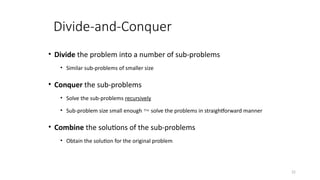
- 22. 22 Divide-and-Conquer • Divide the problem into a number of sub-problems • Similar sub-problems of smaller size • Conquer the sub-problems • Solve the sub-problems recursively • Sub-problem size small enough solve the problems in straightforward manner • Combine the solutions of the sub-problems • Obtain the solution for the original problem
- 23. 23 MergeSort Algorithm MergeSort is a recursive sorting procedure that uses at most O(n*log(n)) comparisons. To sort an array of n elements, we perform the following steps in sequence: If n < 2 then the array is already sorted. Otherwise, n > 1, and we perform the following three steps in sequence: 1. Sort the left half of the the array using MergeSort. 2. Sort the right half of the the array using MergeSort. 3. Merge the sorted left and right halves.
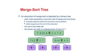
- 24. 24 Merge-Sort Tree An execution of merge-sort is depicted by a binary tree – each node represents a recursive call of merge-sort and stores unsorted sequence before the execution and its partition sorted sequence at the end of the execution – the root is the initial call – the leaves are calls on subsequences of size 0 or 1 7 2 9 4 2 4 7 9 7 2 2 7 9 4 4 9 7 7 2 2 9 9 4 4
- 25. 25 Execution Example Partition 7 2 9 4 3 8 6 1
- 26. 26 Execution Example (cont.) Recursive call, partition 7 2 9 4 7 2 9 4 3 8 6 1
- 27. 27 Execution Example (cont.) Recursive call, partition 7 2 9 4 7 2 7 2 9 4 3 8 6 1
- 28. 28 Execution Example (cont.) Recursive call, base case 7 2 9 4 7 2 7 7 7 2 9 4 3 8 6 1
- 29. 29 Execution Example (cont.) Recursive call, base case 7 2 9 4 7 2 7 7 2 2 7 2 9 4 3 8 6 1
- 30. 30 Execution Example (cont.) Merge 7 2 9 4 7 2 2 7 7 7 2 2 7 2 9 4 3 8 6 1
- 31. 31 Execution Example (cont.) Recursive call, …, base case, merge 7 2 9 4 7 2 2 7 9 4 4 9 7 7 2 2 7 2 9 4 3 8 6 1 9 9 4 4
- 32. 32 Execution Example (cont.) Merge 7 2 9 4 2 4 7 9 7 2 2 7 9 4 4 9 7 7 2 2 9 9 4 4 7 2 9 4 3 8 6 1
- 33. 33 Execution Example (cont.) Recursive call, …, merge, merge 7 2 9 4 2 4 7 9 3 8 6 1 1 3 6 8 7 2 2 7 9 4 4 9 3 8 3 8 6 1 1 6 7 7 2 2 9 9 4 4 3 3 8 8 6 6 1 1 7 2 9 4 3 8 6 1
- 34. 34 Execution Example (cont.) Merge 7 2 9 4 2 4 7 9 3 8 6 1 1 3 6 8 7 2 2 7 9 4 4 9 3 8 3 8 6 1 1 6 7 7 2 2 9 9 4 4 3 3 8 8 6 6 1 1 7 2 9 4 3 8 6 1 1 2 3 4 6 7 8 9
- 35. Complexity Analysis of Merge Sort: •Time Complexity: • Best Case: O(n log n), When the array is already sorted or nearly sorted. • Average Case: O(n log n), When the array is randomly ordered. • Worst Case: O(n log n), When the array is sorted in reverse order.
- 36. Applications, advantages and disadvantages • Applications of Merge Sort: • Sorting large datasets • External sorting (when the dataset is too large to fit in memory) • Inversion counting ( SS SAVED) • It is a preferred algorithm for sorting Linked lists. • It can be easily parallelized as we can independently sort subarrays and then merge.
- 37. Continued • Advantages of Merge Sort: • Stability : Merge sort is a stable sorting algorithm, which means it maintains the relative order of equal elements in the input array. • Simple to implement: The divide-and-conquer approach is straightforward. • Disadvantages of Merge Sort: • Space complexity: Merge sort requires additional memory to store the merged sub-arrays during the sorting process. • Not in-place: Merge sort is not an in-place sorting algorithm, which means it requires additional memory to store the sorted data. This can be a disadvantage in applications where memory usage is a concern. • Slower than QuickSort in general. QuickSort is more cache friendly because it works in- place.
- 38. Merge Algorithm • The basic merging algorithms takes • Two input arrays, A[] and B[], • An output array C[] • And three counters aptr, bptr and cptr. (initially set to the beginning of their respective arrays) • The smaller of A[aptr] and B[bptr] is copied to the next entry in C i.e. C[cptr]. • The appropriate counters are then advanced. • When either of input list is exhausted, the remainder of the other list is copied to C.
- 39. Merge Algorithm 56 66 108 14 A[] aptr 34 12 89 B[] bptr If A[aptr] < B[bptr] C[cptr++] = A[aptr++] Else C[cptr++] = B[bptr++] 14 > 12 therefore C[] cptr C[cptr] = 12 12
- 40. Merge Algorithm 56 66 108 14 A[] aptr 34 12 89 B[] If A[aptr] < B[bptr] C[cptr++] = A[aptr++] Else C[cptr++] = B[bptr++] 14 > 12 therefore cptr++ cptr C[] bptr C[cptr] = 12 12
- 41. Merge Algorithm 56 66 108 14 A[] aptr 34 12 89 B[] If A[aptr] < B[bptr] C[cptr++] = A[aptr++] Else C[cptr++] = B[bptr++] 14 > 12 therefore cptr++ cptr C[] bptr bptr++ C[cptr] = 12 12
- 42. Merge Algorithm 56 66 108 14 A[] aptr 34 12 89 B[] If A[aptr] < B[bptr] C[cptr++] = A[aptr++] Else C[cptr++] = B[bptr++] 14 < 34 therefore cptr C[] bptr 12 C[cptr] = 14 14
- 43. Merge Algorithm 56 66 108 14 A[] aptr 34 12 89 B[] If A[aptr] < B[bptr] C[cptr++] = A[aptr++] Else C[cptr++] = B[bptr++] 14 < 34 therefore cptr++ cptr C[] bptr 12 C[cptr] = 14 14
- 44. Merge Algorithm 56 66 108 14 A[] 34 12 89 B[] If A[aptr] < B[bptr] C[cptr++] = A[aptr++] Else C[cptr++] = B[bptr++] 14 < 34 therefore cptr++ cptr C[] bptr aptr aptr++ 12 C[cptr] = 14 14
- 45. Merge Algorithm 56 66 108 14 A[] aptr 34 12 89 B[] If A[aptr] < B[bptr] C[cptr++] = A[aptr++] Else C[cptr++] = B[bptr++] 56 > 34 therefore cptr C[] bptr 12 14 C[cptr] = 34 34
- 46. Merge Algorithm 56 66 108 14 A[] aptr 34 12 89 B[] If A[aptr] < B[bptr] C[cptr++] = A[aptr++] Else C[cptr++] = B[bptr++] 56 > 34 therefore cptr++ cptr C[] bptr 12 C[cptr] = 34 14 34
- 47. Merge Algorithm 56 66 108 14 A[] aptr 34 12 89 B[] If A[aptr] < B[bptr] C[cptr++] = A[aptr++] Else C[cptr++] = B[bptr++] 56 > 34 therefore cptr++ cptr C[] bptr bptr++ 12 C[cptr] = 34 14 34
- 48. Merge Algorithm 56 66 108 14 A[] aptr 34 12 89 B[] If A[aptr] < B[bptr] C[cptr++] = A[aptr++] Else C[cptr++] = B[bptr++] 56 < 89 therefore cptr C[] bptr 12 14 34 C[cptr] = 56 56
- 49. Merge Algorithm 56 66 108 14 A[] aptr 34 12 89 B[] If A[aptr] < B[bptr] C[cptr++] = A[aptr++] Else C[cptr++] = B[bptr++] 56 < 89 therefore cptr++ cptr C[] bptr 12 14 34 C[cptr] = 56 56
- 50. Merge Algorithm 56 66 108 14 A[] 34 12 89 B[] If A[aptr] < B[bptr] C[cptr++] = A[aptr++] Else C[cptr++] = B[bptr++] 56 < 89 therefore cptr++ cptr C[] bptr aptr aptr++ 12 14 34 C[cptr] = 56 56
- 51. Merge Algorithm 56 66 108 14 A[] 34 12 89 B[] If A[aptr] < B[bptr] C[cptr++] = A[aptr++] Else C[cptr++] = B[bptr++] 66 < 89 therefore cptr C[] bptr aptr 12 14 34 56 C[cptr] = 66 66
- 52. Merge Algorithm 56 66 108 14 A[] 34 12 89 B[] If A[aptr] < B[bptr] C[cptr++] = A[aptr++] Else C[cptr++] = B[bptr++] 66 < 89 therefore cptr++ cptr C[] bptr aptr 12 14 34 C[cptr] = 66 56 66
- 53. Merge Algorithm 56 66 108 14 A[] 34 12 89 B[] If A[aptr] < B[bptr] C[cptr++] = A[aptr++] Else C[cptr++] = B[bptr++] 66 < 89 therefore cptr++ cptr C[] bptr aptr aptr++ 12 14 34 C[cptr] = 66 56 66
- 54. Merge Algorithm 56 66 108 14 A[] 34 12 89 B[] If A[aptr] < B[bptr] C[cptr++] = A[aptr++] Else C[cptr++] = B[bptr++] 108 > 89 therefore cptr C[] bptr aptr 12 14 34 56 66 C[cptr] = 89 89
- 55. Merge Algorithm 56 66 108 14 A[] 34 12 89 B[] If A[aptr] < B[bptr] C[cptr++] = A[aptr++] Else C[cptr++] = B[bptr++] 108 > 89 therefore cptr++ cptr C[] bptr aptr 12 14 34 56 66 C[cptr] = 89 89
- 56. Merge Algorithm 56 66 108 14 A[] 34 12 89 B[] If A[aptr] < B[bptr] C[cptr++] = A[aptr++] Else C[cptr++] = B[bptr++] 108 > 89 therefore cptr++ cptr C[] bptr aptr bptr++ 12 14 34 56 66 C[cptr] = 89 89
- 57. Merge Algorithm 56 66 108 14 A[] 34 12 89 B[] If A[aptr] < B[bptr] C[cptr++] = A[aptr++] Else C[cptr++] = B[bptr++] Array B is now finished, copy remaining elements of array A in array C cptr C[] bptr aptr 12 14 34 56 66 89
- 58. Merge Algorithm 56 66 108 14 A[] 34 12 89 B[] If A[aptr] < B[bptr] C[cptr++] = A[aptr++] Else C[cptr++] = B[bptr++] Array B is now finished, copy remaining elements of array A in array C cptr C[] bptr aptr 12 14 34 56 66 89 108
- 59. 59 Example – n Not a Power of 2 6 2 5 3 7 4 1 6 2 7 4 1 2 3 4 5 6 7 8 9 10 11 q = 6 4 1 6 2 7 4 1 2 3 4 5 6 6 2 5 3 7 7 8 9 10 11 q = 9 q = 3 2 7 4 1 2 3 4 1 6 4 5 6 5 3 7 7 8 9 6 2 10 11 7 4 1 2 2 3 1 6 4 5 4 6 3 7 7 8 5 9 2 10 6 11 4 1 7 2 6 4 1 5 7 7 3 8 Divide
- 60. 60 Example – n Not a Power of 2 7 7 6 6 5 4 4 3 2 2 1 1 2 3 4 5 6 7 8 9 10 11 7 6 4 4 2 1 1 2 3 4 5 6 7 6 5 3 2 7 8 9 10 11 7 4 2 1 2 3 6 4 1 4 5 6 7 5 3 7 8 9 6 2 10 11 2 3 4 6 5 9 2 10 6 11 4 1 7 2 6 4 1 5 7 7 3 8 7 4 1 2 6 1 4 5 7 3 7 8 Conquer and Merge
- 61. 61 Merge- Pseudocode Alg.: MERGE(A, p, q, r) 1. Compute n1 and n2 2. Copy the first n1 elements into L[1 . . n1 + 1] and the next n2 elements into R[1 . . n2 + 1] 3. L[n1 + 1] ← ; R[n2 + 1] ← 4. i 1; j 1 ← ← 5. for k p ← to r 6. do if L[ i ] ≤ R[ j ] 7. then A[k] L[ i ] ← 8. i i + 1 ← 9. else A[k] R[ j ] ← p q 7 5 4 2 6 3 2 1 r q + 1 L R 1 2 3 4 5 6 7 8 6 3 2 1 7 5 4 2 p r q n1 n2
- 62. 62 Merge Sort in C++
- 64. Quick Sort •Fastest known sorting algorithm in practice •Average case: O(N log N) •Worst case: O(N2 ) • But the worst case can be made exponentially unlikely. •Another divide-and-conquer recursive algorithm, like merge sort.
- 65. QuickSort Design • Follows the divide-and-conquer paradigm. • Divide: Partition (separate) the array A[p..r] into two (possibly empty) subarrays A[p..q–1] and A[q+1..r]. • Each element in A[p..q–1] < A[q]. • A[q] < each element in A[q+1..r]. • Index q is computed as part of the partitioning procedure. • Conquer: Sort the two subarrays by recursive calls to quicksort. • Combine: The subarrays are sorted in place – no work is needed to combine them. • How do the divide and combine steps of quicksort compare with those of merge sort?
- 66. Quicksort • If the number of elements in S is 0 or 1, then return (base case). • Divide step: • Pick any element (pivot) v in S • Partition S – {v} into two disjoint groups S1 = {x S – {v} | x <= v} S2 = {x S – {v} | x v} • Conquer step: recursively sort S1 and S2 • Combine step: the sorted S1 (by the time returned from recursion), followed by v, followed by the sorted S2 (i.e., nothing extra needs to be done) v v S1 S2 S To simplify, we may assume that we don’t have repetitive elements, So to ignore the ‘equality’ case!
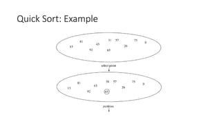
- 68. Example of Quick Sort...
- 69. Pseudocode Quicksort(A, p, r) if p < r then q := Partition(A, p, r); Quicksort(A, p, q – 1); Quicksort(A, q + 1, r) Partition(A, p, r) x, i := A[r], p – 1; for j := p to r – 1 do if A[j] x then i := i + 1; A[i] A[j] A[i + 1] A[r]; return i + 1 5 A[p..r] A[p..q – 1] A[q+1..r] 5 5 Partition 5
- 70. Issues To Consider •How to pick the pivot? • Many methods (discussed later) •How to partition? • Several methods exist. • The one we consider is known to give good results and to be easy and efficient. • We discuss the partition strategy first.
- 71. Partitioning Strategy • For now, assume that pivot = A[(left+right)/2]. • We want to partition array A[left .. right]. • First, get the pivot element out of the way by swapping it with the last element (swap pivot and A[right]). • Let i start at the first element and j start at the next-to-last element (i = left, j = right – 1) pivot i j 5 7 4 6 3 12 19 5 7 4 6 3 12 19 swap
- 72. Partitioning Strategy • Want to have • A[k] pivot, for k < i • A[k] pivot, for k > j • When i < j • Move i right, skipping over elements smaller than the pivot • Move j left, skipping over elements greater than the pivot • When both i and j have stopped • A[i] pivot • A[j] pivot A[i] and A[j] should now be swapped i j 5 7 4 6 3 12 19 i j 5 7 4 6 3 12 19 i j pivot pivot
- 73. Partitioning Strategy (2) • When i and j have stopped and i is to the left of j (thus legal) • Swap A[i] and A[j] • The large element is pushed to the right and the small element is pushed to the left • After swapping • A[i] pivot • A[j] pivot • Repeat the process until i and j cross swap i j 5 7 4 6 3 12 19 i j 5 3 4 6 7 12 19
- 74. Partitioning Strategy (3) • When i and j have crossed • swap A[i] and pivot • Result: • A[k] pivot, for k < i • A[k] pivot, for k > i i j 5 3 4 6 7 12 19 i j 5 3 4 6 7 12 19 i j 5 3 4 6 7 12 19 swap A[i] and pivot Break!
- 75. Picking the Pivot • There are several ways to pick a pivot. • Objective: Choose a pivot so that we will get 2 partitions of (almost) equal size.
- 76. Picking the Pivot (2) • Use the first element as pivot • if the input is random, ok. • if the input is presorted (or in reverse order) • all the elements go into S2 (or S1). • this happens consistently throughout the recursive calls. • results in O(N2 ) behavior (we analyze this case later). • Choose the pivot randomly • generally safe, • but random number generation can be expensive and does not reduce the running time of the algorithm.
- 77. Picking the Pivot (3) • Use the median of the array (ideal pivot) • The N/2 th largest element • Partitioning always cuts the array into roughly half • An optimal quick sort (O(N log N)) • However, hard to find the exact median • Median-of-three partitioning • eliminates the bad case for sorted input.
- 78. Median of Three Method • Compare just three elements: the leftmost, rightmost and center • Swap these elements if necessary so that • A[left] = Smallest • A[right] = Largest • A[center] = Median of three • Pick A[center] as the pivot. • Swap A[center] and A[right – 1] so that the pivot is at the second last position (why?)
- 79. Median of Three: Example pivot 5 6 4 6 3 12 19 2 13 6 5 6 4 3 12 19 2 6 13 A[left] = 2, A[center] = 13, A[right] = 6 Swap A[center] and A[right] 5 6 4 3 12 19 2 13 pivot 6 5 6 4 3 12 19 2 13 Choose A[center] as pivot Swap pivot and A[right – 1] We only need to partition A[ left + 1, …, right – 2 ]. Why?
- 80. Quicksort for Small Arrays • For very small arrays (N<= 20), quicksort does not perform as well as insertion sort • A good cutoff range is N=10 • Switching to insertion sort for small arrays can save about 15% in the running time
- 81. Mergesort vs Quicksort • Both run in O(n*logn) • Mergesort – always. • Quicksort – on average • Compared with Quicksort, Mergesort has less number of comparisons but larger number of moving elements • In Java, an element comparison is expensive but moving elements is cheap. Therefore, Mergesort is used in the standard Java library for generic sorting