Sorting algorithms

Different types of Sorting
Techniques used in Data
Structures And Algorithms

Sorting: Definition
Sorting: an operation that segregates items into groups according to
specified criterion.
A = { 3 1 6 2 1 3 4 5 9 0 }
A = { 0 1 1 2 3 3 4 5 6 9 }

Sorting
• Sorting = ordering.
• Sorted = ordered based on a particular way.
• Generally, collections of data are presented in a sorted
manner.
• Examples of Sorting:
• Words in a dictionary are sorted (and case distinctions are ignored).
• Files in a directory are often listed in sorted order.
• The index of a book is sorted (and case distinctions are ignored).

Review of Complexity
Most of the primary sorting algorithms run on different space and time
complexity.
Time Complexity is defined to be the time the computer takes to run a
program (or algorithm in our case).
Space complexity is defined to be the amount of memory the
computer needs to run a program.

Types of Sorting Algorithms
There are many, many different types of sorting algorithms, but
the primary ones are:

Bubble Sort

Selection Sort

Insertion Sort

Merge Sort

Bubble Sort: Idea
• Idea: bubble in water.
• Bubble in water moves upward. Why?
• How?
• When a bubble moves upward, the water from above will move downward
to fill in the space left by the bubble.

Bubble Sort Example
9, 6, 2, 12, 11, 9, 3, 7
6, 9, 2, 12, 11, 9, 3, 7
6, 2, 9, 12, 11, 9, 3, 7
6, 2, 9, 12, 11, 9, 3, 7
6, 2, 9, 11, 12, 9, 3, 7
6, 2, 9, 11, 9, 12, 3, 7
6, 2, 9, 11, 9, 3, 12, 7
6, 2, 9, 11, 9, 3, 7, 12The 12 is greater than the 7 so they are exchanged.The 12 is greater than the 7 so they are exchanged.
The 12 is greater than the 3 so they are exchanged.The 12 is greater than the 3 so they are exchanged.
The twelve is greater than the 9 so they are exchangedThe twelve is greater than the 9 so they are exchanged
The 12 is larger than the 11 so they are exchanged.The 12 is larger than the 11 so they are exchanged.
In the third comparison, the 9 is not larger than the 12 so no
exchange is made. We move on to compare the next pair without
any change to the list.
In the third comparison, the 9 is not larger than the 12 so no
exchange is made. We move on to compare the next pair without
any change to the list.
Now the next pair of numbers are compared. Again the 9 is the
larger and so this pair is also exchanged.
Now the next pair of numbers are compared. Again the 9 is the
larger and so this pair is also exchanged.
Bubblesort compares the numbers in pairs from left to right
exchanging when necessary. Here the first number is compared
to the second and as it is larger they are exchanged.
Bubblesort compares the numbers in pairs from left to right
exchanging when necessary. Here the first number is compared
to the second and as it is larger they are exchanged.
The end of the list has been reached so this is the end of the first pass. The
twelve at the end of the list must be largest number in the list and so is now in
the correct position. We now start a new pass from left to right.
The end of the list has been reached so this is the end of the first pass. The
twelve at the end of the list must be largest number in the list and so is now in
the correct position. We now start a new pass from left to right.

Bubble Sort Example
6, 2, 9, 11, 9, 3, 7, 122, 6, 9, 11, 9, 3, 7, 122, 6, 9, 9, 11, 3, 7, 122, 6, 9, 9, 3, 11, 7, 122, 6, 9, 9, 3, 7, 11, 12
6, 2, 9, 11, 9, 3, 7, 12
Notice that this time we do not have to compare the last two
numbers as we know the 12 is in position. This pass therefore only
requires 6 comparisons.
Notice that this time we do not have to compare the last two
numbers as we know the 12 is in position. This pass therefore only
First Pass
Second Pass

Bubble Sort Example
2, 6, 9, 9, 3, 7, 11, 122, 6, 9, 3, 9, 7, 11, 122, 6, 9, 3, 7, 9, 11, 12
6, 2, 9, 11, 9, 3, 7, 12
2, 6, 9, 9, 3, 7, 11, 12
Second Pass
First Pass
Third Pass
This time the 11 and 12 are in position. This pass therefore only
This time the 11 and 12 are in position. This pass therefore only

Bubble Sort Example
2, 6, 9, 3, 7, 9, 11, 122, 6, 3, 9, 7, 9, 11, 122, 6, 3, 7, 9, 9, 11, 12
6, 2, 9, 11, 9, 3, 7, 12
2, 6, 9, 9, 3, 7, 11, 12
Second Pass
First Pass
Third Pass
Each pass requires fewer comparisons. This time only 4 are needed.Each pass requires fewer comparisons. This time only 4 are needed.
2, 6, 9, 3, 7, 9, 11, 12Fourth Pass

Bubble Sort Example
2, 6, 3, 7, 9, 9, 11, 122, 3, 6, 7, 9, 9, 11, 12
6, 2, 9, 11, 9, 3, 7, 12
2, 6, 9, 9, 3, 7, 11, 12
Second Pass
First Pass
Third Pass
The list is now sorted but the algorithm does not know this until it
completes a pass with no exchanges.
The list is now sorted but the algorithm does not know this until it
completes a pass with no exchanges.
2, 6, 9, 3, 7, 9, 11, 12Fourth Pass
2, 6, 3, 7, 9, 9, 11, 12Fifth Pass

Bubble Sort Example
2, 3, 6, 7, 9, 9, 11, 12
6, 2, 9, 11, 9, 3, 7, 12
2, 6, 9, 9, 3, 7, 11, 12
Second Pass
First Pass
Third Pass
2, 6, 9, 3, 7, 9, 11, 12Fourth Pass
2, 6, 3, 7, 9, 9, 11, 12Fifth Pass
Sixth Pass
2, 3, 6, 7, 9, 9, 11, 12
This pass no exchanges are made so the algorithm knows the list is
sorted. It can therefore save time by not doing the final pass. With
other lists this check could save much more work.
This pass no exchanges are made so the algorithm knows the list is
sorted. It can therefore save time by not doing the final pass. With
other lists this check could save much more work.

Bubble Sort Example
Questions
1. Which number is definitely in its correct position at the
end of the first pass?
Answer: The last number must be the largest.
Answer: Each pass requires one fewer comparison than the last.
Answer: When a pass with no exchanges occurs.
2. How does the number of comparisons required change as
the pass number increases?
3. How does the algorithm know when the list is sorted?
4. What is the maximum number of comparisons required
for a list of 10 numbers?
Answer: 9 comparisons, then 8, 7, 6, 5, 4, 3, 2, 1 so total 45

Bubble Sort: Example
• Notice that at least one element will be in the correct position each
iteration.
40 2 1 43 3 65 0 -1 58 3 42 4
652 1 40 3 43 0 -1 58 3 42 4
65581 2 3 40 0 -1 43 3 42 4
1 2 3 400 65-1 43 583 42 4
1
2
3
4

1 0 -1 32 653 43 5842404
Bubble Sort: Example
0 -1 1 2 653 43 58424043
-1 0 1 2 653 43 58424043
6
7
8
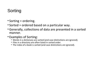
1 2 0 3-1 3 40 6543 584245

Bubble Sort Algorithm
#include<iostream>
using namespace std;
int main(){
//declaring array
int array[5];
cout<<"Enter 5 numbers randomly : "<<endl;
for(int i=0; i<5; i++)
{
//Taking input in array
cin>>array[i];
}
cout<<endl;
cout<<"Input array is: "<<endl;
for(int j=0; j<5; j++)
{
//Displaying Array
cout<<"tttValue at "<<j<<" Index: "<<array[j]<<endl;
}
cout<<endl;

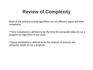
• // Bubble Sort Starts Here
int temp;
for(int i2=0; i2<=4; i2++) // outer loop
{
for(int j=0; j<4; j++) //inner loop
{
//Swapping element in if statement
if(array[j]>array[j+1])
{
temp=array[j];
array[j]=array[j+1];
array[j+1]=temp;
}
}
}
// Displaying Sorted array
cout<<" Sorted Array is: "<<endl;
for(int i3=0; i3<5; i3++)
{
cout<<"tttValue at "<<i3<<" Index: "<<array[i3]<<endl;
}
return 0;
}

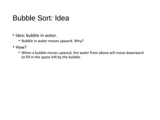
DRY RUN OF CODE
• size of the array is 5 you can change it with your
desired size of array
Input array is
5 4 3 2 -5
so values on indexes of array is
array[0]= 5
array[1]= 4
array[2]= 3
array[3]= 2
array[4]=-5

• In nested for loop bubble sort is doing its work
outer loop variable is i2 will run form 0 to 4
inner loop variable is j will run from 0 to 3
Note for each i2 value inner loop will run from 0 to 3
like when
i2=0 inner loop 0 -> 3

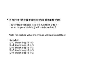
• input 5 4 3 2 -5
for i2= 0;
j=0
array[j]>array[j+1]
5 > 4 if condition true
here we are swapping 4 and 5
array after 4 5 3 2 -5
j=1
array[j]>array[j+1]

• here we are swapping 3 and 5
j=2
array[j]>array[j+1]
here we are swapping 2 and 5
j=3
array[j]>array[j+1]
5 > -5 if condition true

• here we are swapping -5 and 5
array after 4 3 2 -5 5
first iteration completed

Bubble Sort: Analysis
• Running time:
Worst case: O(N2
)
Best case: O(N)

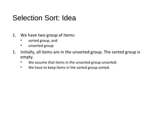
Selection Sort: Idea
1. We have two group of items:
• sorted group, and
• unsorted group
1. Initially, all items are in the unsorted group. The sorted group is
empty.
• We assume that items in the unsorted group unsorted.
• We have to keep items in the sorted group sorted.

Selection Sort: Cont’d
1. Select the “best” (eg. smallest) item from the unsorted group,
then put the “best” item at the end of the sorted group.
2. Repeat the process until the unsorted group becomes empty.

Selection Sort
5 1 3 4 6 2
Comparison
Data Movement
Sorted

Selection Sort
5 1 3 4 6 2
Comparison
Data Movement
Sorted

Largest

Selection Sort
5 1 3 4 2 6
Comparison
Data Movement
Sorted

Selection Sort
5 1 3 4 2 6
Comparison
Data Movement
Sorted

Largest

Selection Sort
2 1 3 4 5 6
Comparison
Data Movement
Sorted

Selection Sort
2 1 3 4 5 6
Comparison
Data Movement
Sorted

Largest

Selection Sort
1 2 3 4 5 6
Comparison
Data Movement
Sorted

Selection Sort
1 2 3 4 5 6
Comparison
Data Movement
Sorted
DONE!

4240 2 1 3 3 4 0 -1 655843
40 2 1 43 3 4 0 -1 42 65583
40 2 1 43 3 4 0 -1 58 3 6542
40 2 1 43 3 65 0 -1 58 3 42 4
Selection Sort: Example

4240 2 1 3 3 4 0 655843-1
42-1 2 1 3 3 4 0 65584340
42-1 2 1 3 3 4 655843400
42-1 2 1 0 3 4 655843403

1
42-1 2 1 3 4 6558434030
42-1 0 3 4 6558434032
1 42-1 0 3 4 6558434032
1 420 3 4 6558434032-1
1 420 3 4 6558434032-1

Algorithm for Selection Sort
void selectionSort(int arr[], int n) {
int i, j, minIndex, tmp;
for (i = 0; i < n - 1; i++) {
minIndex = i;
for (j = i + 1; j < n; j++) {
if (arr[j] < arr[minIndex])
minIndex = j; }
if (minIndex != i) {
tmp = arr[i];
arr[i] = arr[minIndex];
arr[minIndex] = tmp;
}
}
}

Selection Sort: Analysis
• Running time:
Worst case: O(N2
)
Best case: O(N2
)

Insertion Sort: Idea
• Idea: sorting cards.
•8 | 5 9 2 6 3
•5 8 | 9 2 6 3
•5 8 9 | 2 6 3
•2 5 8 9 | 6 3
•2 5 6 8 9 | 3
•2 3 5 6 8 9 |

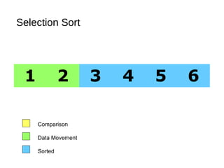
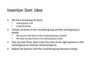
Insertion Sort: Idea
1. We have two group of items:
• sorted group, and
• unsorted group
1. Initially, all items in the unsorted group and the sorted group is
empty.
• We assume that items in the unsorted group unsorted.
• We have to keep items in the sorted group sorted.
1. Pick any item from, then insert the item at the right position in the
sorted group to maintain sorted property.
2. Repeat the process until the unsorted group becomes empty.

40 2 1 43 3 65 0 -1 58 3 42 4
2 40 1 43 3 65 0 -1 58 3 42 4
1 2 40 43 3 65 0 -1 58 3 42 4
40
Insertion Sort: Example

1 2 3 40 43 65 0 -1 58 3 42 4
1 2 40 43 3 65 0 -1 58 3 42 4
1 2 3 40 43 65 0 -1 58 3 42 4

1 2 3 40 43 65 0 -1 58 3 42 4
1 2 3 40 43 650 -1 58 3 42 4
1 2 3 40 43 650 58 3 42 41 2 3 40 43 650-1

1 2 3 40 43 650 58 3 42 41 2 3 40 43 650-1
1 2 3 40 43 650 58 42 41 2 3 3 43 650-1 5840 43 65
1 2 3 40 43 650 42 41 2 3 3 43 650-1 5840 43 65
1 2 3 40 43 650 421 2 3 3 43 650-1 584 43 6542 5840 43 65

Algorithm for Insertion Sort
int a[6] = {5, 1, 6, 2, 4, 3};
int i, j, key;
for(i=1; i<6; i++)
{
key = a[i];
j = i-1;
while(j>=0 && key < a[j])
{
a[j+1] = a[j];
j--;
}
a[j+1] = key;
}

Insertion Sort: Analysis
• Running time analysis:
Worst case: O(N2
)
 Best case: O(N)

Mergesort
•Mergesort (divide-and-conquer)
• Divide array into two halves.
A L G O R I T H M S
divideA L G O R I T H M S

Mergesort
• Recursively sort each half.
sort
A L G O R I T H M S
A G L O R H I M S T

Mergesort
• Recursively sort each half.
• Merge two halves to make sorted whole.
merge
sort
A L G O R I T H M S
A G L O R H I M S T
A G H I L M O R S T

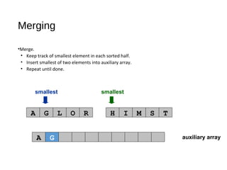
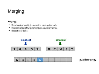
auxiliary array
smallest smallest
A G L O R H I M S T
Merging
•Merge.
• Keep track of smallest element in each sorted half.
• Insert smallest of two elements into auxiliary array.
• Repeat until done.
A

auxiliary array
smallest smallest
A G L O R H I M S T
A
Merging
•Merge.
G

auxiliary array
smallest smallest
A G L O R H I M S T
A G
Merging
•Merge.
H

auxiliary array
smallest smallest
A G L O R H I M S T
A G H
Merging
•Merge.
I

auxiliary array
smallest smallest
A G L O R H I M S T
A G H I
Merging
•Merge.
L

auxiliary array
smallest smallest
A G L O R H I M S T
A G H I L
Merging
•Merge.
M

auxiliary array
smallest smallest
A G L O R H I M S T
A G H I L M
Merging
•Merge.
O

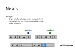
auxiliary array
smallest smallest
A G L O R H I M S T
A G H I L M O
Merging
•Merge.
R

auxiliary array
first half
exhausted smallest
A G L O R H I M S T
A G H I L M O R
Merging
•Merge.
S

auxiliary array
first half
exhausted smallest
A G L O R H I M S T
A G H I L M O R S
Merging
•Merge.
T

Procedure of Merge Sort
Assume, that both arrays are sorted in ascending order and we want
resulting array to maintain the same order. Algorithm to merge two
arrays A[0..m-1] and B[0..n-1] into an array C[0..m+n-1] is as following:
i.Introduce read-indices i, j to traverse arrays A and B, accordingly.
Introduce write-index k to store position of the first free cell in the
resulting array. By default i = j = k = 0.
ii.At each step: if both indices are in range (i < m and j < n), choose
minimum of (A[i], B[j]) and write it to C[k]. Otherwise go to step 4.
iii.Increase k and index of the array, algorithm located minimal value at,
by one. Repeat step 2.
iv.Copy the rest values from the array, which index is still in range, to the
resulting array.

Merge Sort Algorithm
// m - size of A
// n - size of B
// size of C array must be equal or greater than
// m + n
void merge(int m, int n, int A[], int B[], int C[]) {
int i, j, k;
i = 0;
j = 0;
k = 0;

Merge Sort Algorithm Cont..
while (i < m && j < n) {
if (A[i] <= B[j]) {
C[k] = A[i];
i++;
} else {
C[k] = B[j];
j++;
}
k++;
}

Merge Sort Algorithm Cont..
if (i < m) {
for (int p = i; p < m; p++) {
C[k] = A[p];
k++;
}
} else {
for (int p = j; p < n; p++) {
C[k] = B[p];
k++;
}
}
}

Enhancement
• Algorithm could be enhanced in many ways. For instance, it is
reasonable to check, if A[m - 1] < B[0] or B[n - 1] < A[0].
• In any of those cases, there is no need to do more comparisons.
• Algorithm could just copy source arrays in the resulting one in the
right order.
• More complicated enhancements may include searching for
interleaving parts and run merge algorithm for them only. It could
save up much time, when sizes of merged arrays differ in scores of
times.

Time Complexity
• Worst Case Time Complexity : O(n log n)
• Best Case Time Complexity : O(n log n)
• Average Time Complexity : O(n log n)
• Time complexity of Merge Sort is O(n Log n) in all 3 cases (worst,
average and best) as merge sort always divides the array in two
halves and take linear time to merge two halves.

Sorting algorithms

Recommended

More Related Content

What's hot (20)

Viewers also liked (20)

Similar to Sorting algorithms (20)

Recently uploaded (20)

Sorting algorithms