Here are the solutions to the problems:
1. a) Mean = 0.05 rotten tomatoes
b) P(x>1) = 0.03
2. a) Mean = 3.5
b) Variance = 35/12 = 2.91667
c) Standard deviation = 1.7321
3. a) Mean = $0.80
b) Variance = $2.40
4. X Probability
0 1/8
1 3/8
2 3/8
3 1/8
The document discusses the normal curve and standard scores. It defines the normal curve as a continuous probability distribution that is bell-shaped and symmetric. It was developed by Gauss and Pearson. The normal curve can be divided into areas defined by standard deviations from the mean. Standard scores are raw scores converted to other scales, including z-scores, t-scores, and stanines. Z-scores indicate the distance from the mean in standard deviations. T-scores are on a scale of 50 plus or minus 10. Stanines use a nine-point scale with a mean of 5 and standard deviation of 2.
Probability Distribution (Discrete Random Variable)Cess011697
Learning Competencies:
- to find the possible values of a random variable.
illustrates a probability distribution for a discrete random variable and its properties.
- to compute probabilities corresponding to a given random variable.
There are some exercises for you to answer.
Lesson 5: Corpuscles to Chemical Atomic Theory (The Development of Atomic The...Simple ABbieC
At the end of the lesson, you will have to:
1. cite the contribution of John Dalton toward the understanding of the concept of the chemical elements
2. explain how Dalton’s theory contributed to the discovery of other elements.
The document provides information about the Chic'N Poultry Business feasibility study. The business will be located in Bugasong, Antique and will raise broiler chickens for 45 days to produce dressed chicken meat and by-products. It will have 800 broiler chickens. The operational process involves purchasing day-old chicks, feeding them three times a day, vaccination, processing into dressed chicken, and delivery to customers in Bugasong and nearby municipalities. The target market is restaurants, meat shops, and food stalls. The owner aims to be the leading supplier of dressed chicken in the area and increase profits by 5% annually over 5 years.
This document discusses the four levels of measurement: nominal, ordinal, interval, and ratio. Nominal measurement involves using numbers or codes to classify items into categories but does not imply any ordering or mathematical relationships between values. Ordinal measurement allows ranking items but not determining degrees of difference. Interval measurement allows comparing differences but not ratios. Ratio measurement involves true ratios where ratios and zero points have meaningful interpretations. Knowing the level of measurement is important for determining what statistical analyses can be appropriately applied.
This document discusses online platforms and tools that can be used for developing ICT content. It describes different types of online platforms including presentation/visualization tools, cloud computing, social media, file management, mapping, and web page creation tools. It also discusses Google applications such as Docs, Sheets, and Slides that allow online content creation. Basic web design principles and elements like color, layout, links, buttons and images are also covered. The document provides examples of specific online tools for each category like Slideshare, Google Drive, Tumblr and Wix.
Physical and chemical changes of matterMarwa salah
This document discusses physical and chemical changes of matter. It provides examples of physical changes such as melting, dissolving, and grinding, which change a substance's appearance or state but not its chemical composition. Chemical changes, like burning paper or sugar, produce new substances with different properties from the original. The key difference is that physical changes alter appearance or state while chemical changes alter the actual molecular structure and identity of a substance.
This document discusses several key concepts relating to understanding human culture, society, and politics. It addresses objectives around observing cultural variation and differences in human behavior. Some of the main topics covered include defining nationality versus ethnicity, types of gender and socioeconomic class, how political and religious identities can form, and perspectives on cultural relativism. Students are prompted to discuss their own backgrounds and similarities/differences in small groups.
Random Variable (Discrete and Continuous)Cess011697
Learning Competencies
- to recall statistical experiment and sample space
- to illustrate a random variable (discrete and continuous).
- to distinguish between a discrete and a continuous random variable.
The document provides an overview of hypothesis testing, including:
1) The process of hypothesis testing involves deciding between a null and alternative hypothesis based on sample data.
2) The null hypothesis states there is no difference from the claimed population parameter, while the alternative hypothesis states there is a difference.
3) Hypothesis tests use critical values and rejection regions based on the level of significance to determine whether to reject or fail to reject the null hypothesis.
4) Examples are provided to demonstrate conducting hypothesis tests using z-tests and t-tests, and interpreting the results.
This document introduces key concepts related to random variables and probability distributions:
- A random variable is a function that assigns a numerical value to each possible outcome of an experiment. Random variables can be discrete or continuous.
- A probability distribution specifies the possible values of a random variable and their probabilities. For discrete random variables, this is called a probability mass function.
- Key properties of a probability distribution are that each probability is between 0 and 1, and the sum of all probabilities equals 1.
- The mean, variance, and standard deviation can be calculated from a probability distribution. The mean is the expected value, while variance and standard deviation measure dispersion around the mean.
Determining the Mean, Variance, and Standard Deviation of a Discrete Random Variable
Visit the website for more services: https://cristinamontenegro92.wixsite.com/onevs
Rational functions are any functions that can be written as the ratio of two polynomial functions. There are two types of asymptotes for rational functions: vertical asymptotes, which occur at the zeros of the denominator and cannot be crossed, and horizontal asymptotes, which can be crossed. To find the vertical and horizontal asymptotes of a rational function, you examine the degrees of the numerator and denominator polynomials. The domain of a rational function is the set of x-values that make the function defined, while the range is the set of possible y-values produced by the function.
This document discusses constructing probability distributions for discrete random variables. It provides an example of tossing 3 coins and defining the random variable Y as the number of tails. The possible values of Y are 0, 1, 2, and 3 tails. The probabilities of each value are calculated based on the 8 possible outcomes. A probability distribution consists of the random variable values and their probabilities, and it has two key properties: 1) each probability is between 0 and 1, and 2) the sum of all probabilities equals 1.
This document provides an overview of key concepts related to random variables and probability distributions. It discusses:
- Two types of random variables - discrete and continuous. Discrete variables can take countable values, continuous can be any value in an interval.
- Probability distributions for discrete random variables, which specify the probability of each possible outcome. Examples of common discrete distributions like binomial and Poisson are provided.
- Key properties and calculations for discrete distributions like expected value, variance, and the formulas for binomial and Poisson probabilities.
- Other discrete distributions like hypergeometric are introduced for situations where outcomes are not independent. Examples are provided to demonstrate calculating probabilities for each type of distribution.
This document discusses solving rational equations and inequalities. It begins with definitions of rational equations and inequalities. Examples are provided to demonstrate how to solve rational equations by multiplying both sides by the least common denominator to eliminate fractions. The document notes that extraneous solutions may arise and must be checked. Methods for solving rational inequalities using graphs, tables, and algebra are presented. Practice problems are included for students to test their understanding.
This document discusses rational functions and their graphs. It defines a rational function as a function of the form f(x) = p(x)/q(x) where p and q are polynomials. It explains that the domain of a rational function excludes any values that would make the denominator equal to 0. It describes how to find vertical, horizontal, and oblique asymptotes of a rational function by comparing the degrees of the polynomials in the numerator and denominator. Vertical asymptotes occur where the denominator is 0, and horizontal or oblique asymptotes depend on whether the degree of the numerator is less than, equal to, or greater than the degree of the denominator. Examples are provided to illustrate these concepts.
The document discusses inverse functions and how an inverse function undoes the operations of the original function. It provides examples of finding the inverse of functions by switching the x and y values and solving for y. The inverse of a function will be a function itself only if the original function passes the horizontal line test.
This document discusses graphing rational functions. It defines key concepts like domain, range, intercepts, zeros, and asymptotes. An example rational function f(x)=x-2/(x+2) is used to demonstrate how to find these values and graph the function. The domain is all real numbers except -2, the x-intercept is 2, and the y-intercept is -1. The vertical asymptote is at x=-2. Horizontal asymptotes occur when the degree of the numerator is less than, equal to, or greater than the degree of the denominator.
Please Subscribe to this Channel for more solutions and lectures
http://www.youtube.com/onlineteaching
Chapter 5: Discrete Probability Distribution
5.1: Probability Distribution
The document provides information and examples about solving rational equations. It discusses that a rational equation contains one or more rational expressions. It then provides two main methods for solving rational equations - cross multiplying and finding the least common denominator. Several steps are outlined for using the least common denominator method, including finding the common denominator, clearing denominators by multiplying both sides by the LCM, solving the resulting equation, and checking solutions. Examples of using both methods to solve rational equations are shown. Additional resources for learning more about solving rational equations are also provided.
If you are looking for math video tutorials (with voice recording), you may download it on our YouTube Channel. Don't forget to SUBSCRIBE for you to get updated on our upcoming videos.
https://tinyurl.com/y9muob6q
Also, please do visit our page, LIKE and FOLLOW us on Facebook!
https://tinyurl.com/ycjp8r7u
https://tinyurl.com/ybo27k2u
This document discusses estimating population parameters from sample statistics. It defines a point estimate of the population mean as the mean of sample means. The document provides an example where a consumer group took random samples of bottle capacities to estimate the true population mean capacity claimed by a company. It demonstrates computing the mean of each sample and the point estimate of the population mean. Finally, it provides formulas for computing variance and standard deviation as other measures of the population from sample statistics.
Chapter 4 part3- Means and Variances of Random Variablesnszakir
Statistics, study of probability, The Mean of a Random Variable, The Variance of a Random Variable, Rules for Means and Variances, The Law of Large Numbers,
Mean and Variance of Discrete Random Variable.pptxMarkJayAquillo
The document discusses computing the mean, variance, and standard deviation of discrete random variables. It provides examples of calculating the mean of different probability distributions by taking the sum of each value multiplied by its probability. It also gives examples of finding variance by taking the sum of the squared differences between each value and the mean multiplied by its probability, and defines standard deviation as the square root of variance. The document aims to help readers understand how to calculate and interpret these statistical measures for discrete random variables.
Probability Distributions for Discrete Variablesgetyourcheaton
This document discusses probability distributions for discrete variables. It begins by defining a probability distribution as a relative frequency distribution of all possible outcomes of an experiment. It provides examples of probability distributions for discrete variables like the binomial distribution. It discusses key aspects of probability distributions like the mean, standard deviation, and different types of distributions like binomial. It provides examples of calculating probabilities, means, and standard deviations for binomial distributions. It discusses the basic characteristics of the binomial distribution and provides an example of constructing a binomial distribution and calculating related probabilities.
Random variables can be either discrete or continuous. A discrete random variable takes on countable values, while a continuous random variable can take on any value within a range. The probability distributions for discrete and continuous random variables are different. A discrete probability distribution lists each possible value and its probability, while a continuous distribution is described using a probability density function. Random variables are used widely in statistics and probability to model outcomes of experiments and random phenomena.
This document contains a lesson plan on probability for students. It begins with definitions of key probability terms and examples of calculating probabilities of simple and compound events. It then provides word problems for students to practice calculating probabilities. The document concludes with additional practice problems for students to answer. The overall document provides instruction and practice on fundamental concepts in probability.
This document provides an overview of random variables and probability distributions. It defines discrete and continuous random variables and gives examples of each. Discrete random variables have probabilities associated with each possible value, while continuous random variables are defined by probability density functions where the area under the curve equals the probability. The document discusses how to calculate the mean, variance and standard deviation of discrete random variables from their probability distributions. It also covers how the mean and variance are affected for linear transformations of random variables.
This document discusses several discrete probability distributions:
1. Binomial distribution - For experiments with a fixed number of trials, two possible outcomes, and constant probability of success. The probability of x successes is given by the binomial formula.
2. Geometric distribution - For experiments repeated until the first success. The probability of the first success on the xth trial is p(1-p)^(x-1).
3. Poisson distribution - For counting the number of rare, independent events occurring in an interval. The probability of x events is (e^-μ μ^x)/x!, where μ is the mean number of events.
Probability and Statistics : Binomial Distribution notes ppt.pdfnomovi6416
This document provides an overview of several discrete probability distributions:
- The discrete uniform distribution where each value has an equal probability of 1/k.
- The binomial distribution which models the number of successes in n independent yes/no trials with probability of success p.
- The hypergeometric distribution which models sampling without replacement from a finite population.
- The Poisson distribution which models the number of rare, independent events occurring in a fixed interval of time or space with a constant average rate λ.
Formulas are given for the probability mass functions and key properties like the mean and variance of each distribution. Examples are provided to illustrate calculating probabilities and distribution parameters.
2 DISCRETE PROBABILITY DISTRIBUTION.pptxRYANCENRIQUEZ
The document discusses discrete probability distributions and provides examples of constructing probability distributions for random variables. A discrete probability distribution lists each possible value a random variable can take and its probability. It must have probabilities between 0 and 1 that sum to 1. Examples include coin flips and dice rolls. The document also provides practice problems for constructing probability distributions and determining if a distribution represents a discrete random variable.
GROUP 4 IT-A.pptx ptttt ppt ppt ppt ppt ppt pptZainUlAbedin85
This document discusses discrete random variables and their probability distributions. It defines a discrete random variable as one that has a finite or countable number of possible outcomes that can be listed. It provides examples of discrete and continuous random variables. It then explains how to construct a probability distribution for a discrete random variable by listing the possible outcomes and their probabilities, ensuring the probabilities sum to 1. It also covers how to graph a discrete probability distribution, calculate the mean, variance, and standard deviation of a discrete random variable from its probability distribution.
The document discusses random variables and probability distributions. It defines a random variable as a function that assigns a numerical value to each outcome in a sample space. Random variables can be discrete or continuous. The probability distribution of a random variable describes its possible values and the probabilities associated with each value. It then discusses the binomial distribution in detail as an example of a theoretical probability distribution. The binomial distribution applies when there are a fixed number of independent yes/no trials, each with the same constant probability of success.
Probability theory discrete probability distributionsamarthpawar9890
This document provides an overview of discrete probability distributions and binomial distributions. It begins by defining random variables and describing discrete and continuous random variables. Examples are given to distinguish between the two. The key aspects of discrete probability distributions are outlined, including how to construct a distribution and calculate measures such as mean, variance, and standard deviation. Binomial experiments are defined as having two possible outcomes, a fixed number of trials, and constant probability of success. The binomial probability formula is presented and used to calculate probabilities in examples.
ISM_Session_5 _ 23rd and 24th December.pptxssuser1eba67
The document discusses random variables and their probability distributions. It defines discrete and continuous random variables and their key characteristics. Discrete random variables can take on countable values while continuous can take any value in an interval. Probability distributions describe the probabilities of a random variable taking on different values. The mean and variance are discussed as measures of central tendency and variability. Joint probability distributions are introduced for two random variables. Examples and homework problems are also provided.
This document provides an overview of random variables and various discrete probability distributions. It defines random variables and describes discrete and continuous random variables. It also covers the mean, variance, and standard deviation of discrete random variables. Various discrete probability distributions are introduced, including the discrete uniform distribution, Bernoulli distribution, and binomial distribution. Examples are provided to illustrate key concepts.
The document discusses different types of discrete probability distributions:
- Uniform distribution where all outcomes are equally likely, like when rolling a fair die.
- Bernoulli distribution which has only two possible outcomes (success/failure) with probabilities p and q=1-p.
- Binomial distribution which describes experiments with a fixed number of trials, two possible outcomes per trial (success/failure), and where trials are independent with constant probability of success p.
Here are the probabilities of the given events:
a) Getting an odd number in a single roll of a die: 1/2
b) Getting an ace when a card is drawn from a deck: 4/52
c) Getting a number greater than 2 in a single roll of a die: 3/6 = 1/2
d) Getting a red queen when a card is drawn from a deck: 1/52
e) Getting doubles when two dice are rolled: 1/6
This document defines discrete and continuous random variables and provides examples of each. It then focuses on discrete random variables and probability distributions. Specifically, it discusses the binomial probability distribution, giving its formula and providing examples of calculating binomial probabilities. It also discusses properties of the binomial distribution such as its shape and mean, and shows how binomial tables can be used to find probabilities.
Form View Attributes in Odoo 18 - Odoo SlidesCeline George
Odoo is a versatile and powerful open-source business management software, allows users to customize their interfaces for an enhanced user experience. A key element of this customization is the utilization of Form View attributes.
This chapter provides an in-depth overview of the viscosity of macromolecules, an essential concept in biophysics and medical sciences, especially in understanding fluid behavior like blood flow in the human body.
Key concepts covered include:
✅ Definition and Types of Viscosity: Dynamic vs. Kinematic viscosity, cohesion, and adhesion.
⚙️ Methods of Measuring Viscosity:
Rotary Viscometer
Vibrational Viscometer
Falling Object Method
Capillary Viscometer
🌡️ Factors Affecting Viscosity: Temperature, composition, flow rate.
🩺 Clinical Relevance: Impact of blood viscosity in cardiovascular health.
🌊 Fluid Dynamics: Laminar vs. turbulent flow, Reynolds number.
🔬 Extension Techniques:
Chromatography (adsorption, partition, TLC, etc.)
Electrophoresis (protein/DNA separation)
Sedimentation and Centrifugation methods.
Title: A Quick and Illustrated Guide to APA Style Referencing (7th Edition)
This visual and beginner-friendly guide simplifies the APA referencing style (7th edition) for academic writing. Designed especially for commerce students and research beginners, it includes:
✅ Real examples from original research papers
✅ Color-coded diagrams for clarity
✅ Key rules for in-text citation and reference list formatting
✅ Free citation tools like Mendeley & Zotero explained
Whether you're writing a college assignment, dissertation, or academic article, this guide will help you cite your sources correctly, confidently, and consistent.
Created by: Prof. Ishika Ghosh,
Faculty.
📩 For queries or feedback: [email protected]
What is the Philosophy of Statistics? (and how I was drawn to it)jemille6
What is the Philosophy of Statistics? (and how I was drawn to it)
Deborah G Mayo
At Dept of Philosophy, Virginia Tech
April 30, 2025
ABSTRACT: I give an introductory discussion of two key philosophical controversies in statistics in relation to today’s "replication crisis" in science: the role of probability, and the nature of evidence, in error-prone inference. I begin with a simple principle: We don’t have evidence for a claim C if little, if anything, has been done that would have found C false (or specifically flawed), even if it is. Along the way, I’ll sprinkle in some autobiographical reflections.
This slide is an exercise for the inquisitive students preparing for the competitive examinations of the undergraduate and postgraduate students. An attempt is being made to present the slide keeping in mind the New Education Policy (NEP). An attempt has been made to give the references of the facts at the end of the slide. If new facts are discovered in the near future, this slide will be revised.
This presentation is related to the brief History of Kashmir (Part-I) with special reference to Karkota Dynasty. In the seventh century a person named Durlabhvardhan founded the Karkot dynasty in Kashmir. He was a functionary of Baladitya, the last king of the Gonanda dynasty. This dynasty ruled Kashmir before the Karkot dynasty. He was a powerful king. Huansang tells us that in his time Taxila, Singhpur, Ursha, Punch and Rajputana were parts of the Kashmir state.
How to Create A Todo List In Todo of Odoo 18Celine George
In this slide, we’ll discuss on how to create a Todo List In Todo of Odoo 18. Odoo 18’s Todo module provides a simple yet powerful way to create and manage your to-do lists, ensuring that no task is overlooked.
Happy May and Happy Weekend, My Guest Students.
Weekends seem more popular for Workshop Class Days lol.
These Presentations are timeless. Tune in anytime, any weekend.
<<I am Adult EDU Vocational, Ordained, Certified and Experienced. Course genres are personal development for holistic health, healing, and self care. I am also skilled in Health Sciences. However; I am not coaching at this time.>>
A 5th FREE WORKSHOP/ Daily Living.
Our Sponsor / Learning On Alison:
Sponsor: Learning On Alison:
— We believe that empowering yourself shouldn’t just be rewarding, but also really simple (and free). That’s why your journey from clicking on a course you want to take to completing it and getting a certificate takes only 6 steps.
Hopefully Before Summer, We can add our courses to the teacher/creator section. It's all within project management and preps right now. So wish us luck.
Check our Website for more info: https://ldmchapels.weebly.com
Get started for Free.
Currency is Euro. Courses can be free unlimited. Only pay for your diploma. See Website for xtra assistance.
Make sure to convert your cash. Online Wallets do vary. I keep my transactions safe as possible. I do prefer PayPal Biz. (See Site for more info.)
Understanding Vibrations
If not experienced, it may seem weird understanding vibes? We start small and by accident. Usually, we learn about vibrations within social. Examples are: That bad vibe you felt. Also, that good feeling you had. These are common situations we often have naturally. We chit chat about it then let it go. However; those are called vibes using your instincts. Then, your senses are called your intuition. We all can develop the gift of intuition and using energy awareness.
Energy Healing
First, Energy healing is universal. This is also true for Reiki as an art and rehab resource. Within the Health Sciences, Rehab has changed dramatically. The term is now very flexible.
Reiki alone, expanded tremendously during the past 3 years. Distant healing is almost more popular than one-on-one sessions? It’s not a replacement by all means. However, its now easier access online vs local sessions. This does break limit barriers providing instant comfort.
Practice Poses
You can stand within mountain pose Tadasana to get started.
Also, you can start within a lotus Sitting Position to begin a session.
There’s no wrong or right way. Maybe if you are rushing, that’s incorrect lol. The key is being comfortable, calm, at peace. This begins any session.
Also using props like candles, incenses, even going outdoors for fresh air.
(See Presentation for all sections, THX)
Clearing Karma, Letting go.
Now, that you understand more about energies, vibrations, the practice fusions, let’s go deeper. I wanted to make sure you all were comfortable. These sessions are for all levels from beginner to review.
Again See the presentation slides, Thx.
A measles outbreak originating in West Texas has been linked to confirmed cases in New Mexico, with additional cases reported in Oklahoma and Kansas. The current case count is 817 from Texas, New Mexico, Oklahoma, and Kansas. 97 individuals have required hospitalization, and 3 deaths, 2 children in Texas and one adult in New Mexico. These fatalities mark the first measles-related deaths in the United States since 2015 and the first pediatric measles death since 2003.
The YSPH Virtual Medical Operations Center Briefs (VMOC) were created as a service-learning project by faculty and graduate students at the Yale School of Public Health in response to the 2010 Haiti Earthquake. Each year, the VMOC Briefs are produced by students enrolled in Environmental Health Science Course 581 - Public Health Emergencies: Disaster Planning and Response. These briefs compile diverse information sources – including status reports, maps, news articles, and web content– into a single, easily digestible document that can be widely shared and used interactively. Key features of this report include:
- Comprehensive Overview: Provides situation updates, maps, relevant news, and web resources.
- Accessibility: Designed for easy reading, wide distribution, and interactive use.
- Collaboration: The “unlocked" format enables other responders to share, copy, and adapt seamlessly. The students learn by doing, quickly discovering how and where to find critical information and presenting it in an easily understood manner.
CURRENT CASE COUNT: 817 (As of 05/3/2025)
• Texas: 688 (+20)(62% of these cases are in Gaines County).
• New Mexico: 67 (+1 )(92.4% of the cases are from Eddy County)
• Oklahoma: 16 (+1)
• Kansas: 46 (32% of the cases are from Gray County)
HOSPITALIZATIONS: 97 (+2)
• Texas: 89 (+2) - This is 13.02% of all TX cases.
• New Mexico: 7 - This is 10.6% of all NM cases.
• Kansas: 1 - This is 2.7% of all KS cases.
DEATHS: 3
• Texas: 2 – This is 0.31% of all cases
• New Mexico: 1 – This is 1.54% of all cases
US NATIONAL CASE COUNT: 967 (Confirmed and suspected):
INTERNATIONAL SPREAD (As of 4/2/2025)
• Mexico – 865 (+58)
‒Chihuahua, Mexico: 844 (+58) cases, 3 hospitalizations, 1 fatality
• Canada: 1531 (+270) (This reflects Ontario's Outbreak, which began 11/24)
‒Ontario, Canada – 1243 (+223) cases, 84 hospitalizations.
• Europe: 6,814
How to Clean Your Contacts Using the Deduplication Menu in Odoo 18Celine George
In this slide, we’ll discuss on how to clean your contacts using the Deduplication Menu in Odoo 18. Maintaining a clean and organized contact database is essential for effective business operations.
Ajanta Paintings: Study as a Source of HistoryVirag Sontakke
This Presentation is prepared for Graduate Students. A presentation that provides basic information about the topic. Students should seek further information from the recommended books and articles. This presentation is only for students and purely for academic purposes. I took/copied the pictures/maps included in the presentation are from the internet. The presenter is thankful to them and herewith courtesy is given to all. This presentation is only for academic purposes.
Computer crime and Legal issues Computer crime and Legal issuesAbhijit Bodhe
• Computer crime and Legal issues: Intellectual property.
• privacy issues.
• Criminal Justice system for forensic.
• audit/investigative.
• situations and digital crime procedure/standards for extraction,
preservation, and deposition of legal evidence in a court of law.
8. Random Variable
-assigns a number to each
outcome of a random
circumstance, or,
equivalently, to each unit in
a population.
-is a number generated by a
random experiment
9. Two different types of random variables:
*1. A continuous random variable can take
any value in an interval or collection of
intervals. Its possible values contain a
whole interval of numbers.
*2. A discrete random variable can take one
of a countable list of distinct values. Its
possible values form a finite or countable
set.
*Notation for either type: X, Y, Z, W, etc.
10. Examples of Discrete Random Variables Assigns a
number to each outcome in the sample space for a
random circumstance, or to each unit in a
population.
1. Couple plans to have 3 children. The random
circumstance includes the 3 births, specifically
the sexes of the 3 children. Possible outcomes
(sample space): BBB, BBG, etc.
X = number of girls
X is discrete and can be 0, 1, 2, 3
For example, the number assigned to BBB is X=0
2. Population consists of students (unit = student)
Y = number of siblings a student has
Y is discrete and can be 0, 1, 2, …??
11. Examples of Continuous Random Variables
Assigns a number to each outcome of a
random circumstance, or to each unit in a
population.
1.Population consists of female students
Unit = female student
W = height
W is continuous – can be anything in an
interval, even if we report it to nearest inch or
half inch
2. You are waiting at a bus stop for the next bus
Random circumstance = when the bus arrives
Y = time you have to wait
Y is continuous – anything in an interval
12. 2 TYPES OF RANDOM VARIABLES
DISCRETE RANDOM VARIABLES
Number of scales
Number of calls
People in a line
Score in an exam
CONTINUOUS RANDOM VARIABLES
Length
Depth
Volume
Time
Weight
13. EXPERIMENT RANDOM VARIABLE POSSIBLE VALUES
of X
Roll two fair dice X=Sum of the
number of dots on
the top face
2, 3, 4, 5, 6, 7, 8,
9, 10, 11, 12
Flip a fair coin
repeatedly
X=Number of
tosses until the
coin lands heads
1, 2, 3, 4, …
Measure of voltage
at an electrical
outlet
X=Voltage
measured
118<x<122
The air pressure of
a tire on an
automobile
X=Air pressure 30<x<32
14. Classify each random variable as either
discrete or continuous.
1.The number of arrivals a an emergency
room between midnight and 6:00 a.m.
2.The weight of a box of cereal
3.The duration of the next outgoing call
from a business office
4.The number of boys in a randomly
selected thee-child policy
5.The temperature of a cup of coffee
served at a restaurant.
15. Classify each random variable as either
discrete or continuous.
1. The number of applicants in a job
2. The time between customers
entering a checkout lane at a retail
store.
3. The average amount of electricity a
household consume in a month
4. The number of accident-free days
in one month at a factory
5. The number of vehicles owned by a
government official
16. The number of heads in two tosses
of a coin
The average weight of newborn
babies in the Philippines
The number of games in the
basketball boys of junior high
The number of coins that match
when three coins are tossed at once
Identify the set of possible values for each
random variable.
18. What is the probability of getting
a head in a toss of a coin
What is the pro babilityof getting
a Queen of Heart ♥ in a deck of
cards?
What is the probability of a
female Grade 11 Stem Student to
be chosen from their section?
19. Probability Distributions
Of a discrete random
variable X is a list of each
possible value of X
together with the
probability that X takes
that value in one trial of
the experiment
20. The probabilities in the probability distribution of a
random variable X must satisfy the following two
conditions:
1. Each probability P (x) must be
between 0 and 1:
0 ≤ P (x) ≤ 1.
2. The sum of all the probabilities is 1:
ΣP(x) = 1.
21. EXAMPLE 1
A fair coin is tossed twice. Let X be the number of heads
that are observed.
a. Construct the probability distribution of X.
b. Find the probability that at least one head is observed.
Solution:
a. The possible values that X can take are 0, 1, and 2. Each of
these numbers corresponds to an event in the sample space
S = {hh, ht, th, tt} of equally likely outcomes for this
experiment: X = 0 to {tt}, X = 1 to {ht, th} , and X = 2 to
{hh}. The probability of each of these events, hence of the
corresponding value of X, can be found simply by counting,
to give x 0 1 2
P(x) ¼ or 0.25 2/4 or 0.50 ¼ or 0.25
This table is the probability distribution of X.
22. A histogram that graphically
illustrates the probability
distribution is given in Figure 4.1
"Probability Distribution for
Tossing a Fair Coin Twice".
23. EXAMPLE 2
A pair of fair dice is rolled. Let X denote the sum of the
number of dots on the top faces.
a. Construct the probability distribution of X.
b. Find P(X ≥ 9).
c. Find the probability that X takes an even value.
Solution:
The sample space of equally likely outcomes is
11 12 13 14 15 16
21 22 23 24 25 26
31 32 33 34 35 36
41 42 43 44 45 46
51 52 53 54 55 56
61 62 63 64 65 66
24. This table is the probability distribution of X.
a. The possible values for X are the numbers 2 through 12.
X = 2 is the event {11}, so P (2) =
1
36
.
X = 3 is the event {12,21}, so P (3) =
2
36
.
Continuing this way we obtain the table
x 2 3 4 5 6 7 8 9 10 11 12
P(x) 1
36
2
36
3
36
4
36
5
36
6
36
5
36
4
36
3
36
2
36
1
36
25. b. The event X ≥ 9 is the union of the mutually exclusive
events X =9, X = 10, X = 11, and X = 12. Thus
P (X ≥ 9) = P(9) +P(10) +P(11) +P(12)
=
𝟒
𝟑𝟔
+
𝟑
𝟑𝟔
+
𝟐
𝟑𝟔
+
𝟏
𝟑𝟔
=
𝟓
𝟏𝟖
c. Note that X takes six different even values but only five
different odd values. We compute
P(X is even)=P(2)+ P(4)+ P(6)+ P(8)+ P(10)+ P(12)
=
𝟏
𝟑𝟔
+
𝟑
𝟑𝟔
+
𝟓
𝟑𝟔
+
𝟓
𝟑𝟔
+
𝟑
𝟑𝟔
+
𝟏
𝟑𝟔
=
𝟏𝟖
𝟑𝟔
or 0.5
x 2 3 4 5 6 7 8 9 10 11 12
P(x) 1
36
2
36
3
36
4
36
5
36
6
36
5
36
4
36
3
36
2
36
1
36
26. A histogram that graphically
illustrates the probability
distribution is given in Figure 4.2
"Probability Distribution for
Tossing Two Fair Dice".
27. Determine whether or not the table is a valid
probability distribution of a discrete random
variable.
x -2 0 2 4
P(x) 0.3 0.5 0.2 0.1
X 0.5 0.25 0.25
P(x) -0.4 0.6 0.8
A discrete random variable X has the
following probability distribution:
x 77 78 79 80 81
P(x) 0.15 0.15 0.20 0.40 0.10
Compute each of the following quantities.
a. P (80)
b. P(X > 80)
c. P(X ≤ 80)
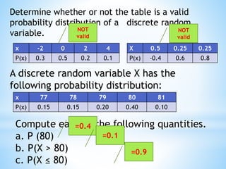
28. Determine whether or not the table is a valid
probability distribution of a discrete random
variable.
x -2 0 2 4
P(x) 0.3 0.5 0.2 0.1
X 0.5 0.25 0.25
P(x) -0.4 0.6 0.8
A discrete random variable X has the
following probability distribution:
x 77 78 79 80 81
P(x) 0.15 0.15 0.20 0.40 0.10
Compute each of the following quantities.
a. P (80)
b. P(X > 80)
c. P(X ≤ 80)
NOT
valid
NOT
valid
=0.4
=0.1
=0.9
29. Learning Competency:
Illustrates the mean, variance &
standard deviation of a discrete random
variable
Calculates the mean, variance &
standard deviation of a discrete random
variable
*
30. Definition
The mean (also called the
expected value) of a discrete random
variable X is the number
μ = Σ [x·P(x)]
The mean of a random variable may be
interpreted as the average of the
values assumed by the random variable
in repeated trials of the experiment.
31. EXAMPLE
Find the mean of the discrete random
variable X whose probability
distribution is
x -2 1 2 3.5
P(x) 0.21 0.34 0.24 0.21
Solution:
The formula in the definition gives
μ =Σx P(x)
=(−2) · 0.21 + (1) · 0.34 + (2) · 0.24 +(3.5)· 0.21
= 1.135
32. Definition
The variance, σ2, of a discrete
random variable X is the
number σ2= Σ(x − μ)2P(x)
which by algebra is equivalent
to the formula
σ2=[Σ x2P(x)]−μ2
33. Definition
The standard deviation , σ, of a discrete
random variable X is the square root of its
variance, hence is given by the formula
σ = 𝝈 𝟐
The variance and standard deviation of a
discrete random variable X may be
interpreted as measures of the variability of
the values assumed by the random variable
in repeated trials of the experiment. The
units on the standard deviation match those
of X.
34. EXAMPLE
Find the variance and standard deviation
of the discrete random variable X whose
probability distribution is
X -1 0 1 4
P(x) 0.2 0.5 0.2 0.1
Compute each of the following quantities.
a. The mean μ of X.
b. The variance σ2 of X.
c. The standard deviation σ of X.
35. Solution:
a.Using the formula in the definition of μ,
μ = Σx P (x)
= (−1) · 0.2 + 0 · 0.5 + 1 · 0.2 + 4 · 0.1
= 0.4
b. Using the formula in the definition of σ2 and
the value of μ that was just computed,
σ2=[Σ x2P(x)]−μ2
= [(−1)2 ·0.2 + 02 ·0.5 + 12 ·0.2 + 42 ·0.1]-0.42
=1.84
c. Using the result of b,
σ = 1.84
= 1.3565
36. A discrete random variable X has the
following probability distribution:
x 77 78 79 80 81
P(x) 0.15 0.15 0.20 0.40 0.10
Compute each of the following quantities.
a. The mean μ of X.
b. The variance σ2 of X.
f. The standard deviation σ of X.
37. A discrete random variable X has the
following probability distribution:
x 77 78 79 80 81
P(x) 0.15 0.15 0.20 0.40 0.10
Compute each of the following quantities.
a. The mean μ of X. ans.=79.15
b. The variance σ2 of X. ans.=1.5275
f. The standard deviation σ of X. ans.=1.24
38. Two fair dice are rolled
at once. Let X denote
the difference in the
number of dots that
appear on the top faces
of the two dice. Thus for
example if a one and a
five are rolled, X = 4,
and if two sixes are
rolled, X = 0.
a. Construct the
probability
distribution for X.
b. Compute the
mean μ of X.
c. Compute the
standard deviation σ
of X.
41. TEST I. Solve the following:
1. A grocery store has determined that
in crates of tomatoes, 95% carry no
rotten tomatoes, 2% carry one rotten
tomato, 2% carry two rotten tomatoes,
and 1% carry three rotten tomatoes.
a. Find the mean number of rotten tomatoes in the
crates.”
b. What is P(x>1)?
42. 2. Probability distribution
that results from the rolling
of a single fair die.
x 1 2 3 4 5 6
p(x) 1/6 1/6 1/6 1/6 1/6 1/6
Compute each of the following
quantities.
a. The mean μ of X.
b. The variance σ2 of X.
c. The standard deviation σ of X.
43. 3. Suppose an individual plays a gambling
game where it is possible to lose $1.00,
break even, win $3.00, or win $10.00
each time she plays. The probability
distribution for each outcome is provided
by the following table:
Outcome -$1.00 $0.00 $3.00 $5.00
Probability 0.30 0.40 0.20 0.10
a. Find the mean
b. Find the variance.
44. 4. Let X denote the number of boys
in a randomly selected three-child
family. Assuming that boys and girls
are equally likely, construct the
probability distribution of X.
5. Let X denote the number of times
a fair coin lands heads in three
tosses. Construct the probability
distribution of X.
45. TEST II. Identify the following
variables(DISCRETE OR CONTINUOUS):
1. distance traveled between classes
2. number of students present
3. height of students in class
4. number of red marbles in a jar
5. time it takes to get to school
6. number of heads when flipping three coins
7. students’ grade level
8. The temperature of a cup of coffee served
at a restaurant
9. The number of applicants for a job.
10.weight of students in class
46. TEST III. Determine whether or not the table is a
valid probability distribution of a discrete
random variable.
1.
2.
3.
4.
5.
x -2 0 2 4
P(x) 0.4 0.5 0.1 0.1
X 0.5 0.25 0.25
P(x) 0.2 0.6 0.2
x 5 6 7 8
P(x) -0.1 0.5 0.4 0.2
X -4 -3 -2 -1
P(x) 0.25 0.20 0.40 0.15
X 1 2 3 4
P(x) ¼ ¼ ¼ ¼
47. 1. a. 0.09 b. 0.03
2. a. 7/2 b. 2.92
c. 1.71
3. a. 0.8b. 3.36
c. 1.83
49. 1. Let X denote the number of times
a fair coin lands heads in three
tosses. Construct the probability
distribution of X.
50. 2. Probability distribution
that results from the rolling
of a single fair die.
x 1 2 3 4 5 6
p(x) 1/6 1/6 1/6 1/6 1/6 1/6
Compute each of the following
quantities.
a. The mean μ of X.
b. The variance σ2 of X.
c. The standard deviation σ of X.