


![Spark및Kafka를이용한빅데이터실시간처리기술
Spark & RDD?
• RDD
• Spark 에서의 기본형
• 특징
• Dependencies
• Partitions (with some locality information)
• Compute function: Partition => Iterator[T]
• 단, original model에서의 문제
• (i) compute function is opaque to Spark. Spark only sees it as a lambda expression.
• (ii) Iterator[T] data type is also opaque for Python RDDs.
• (iii) Spark has no way to optimize the expression
• (iv) Spark has no knowledge of specific data type in T.](https://image.slidesharecdn.com/sparkandkafkaaf-240509080607-24967ade/85/Streaming-using-Spark-and-Kafka-36-320.jpg)
![Spark및Kafka를이용한빅데이터실시간처리기술
Structuring Spark
• 장점
• Low-level RDD API vs. high-level DSL
# In Python
# Create an RDD of tuples (name, age)
dataRDD = sc.parallelize([("Brooke", 20), ("Denny", 31),
("Jules", 30),
("TD", 35), ("Brooke", 25)])
# Use map and reduceByKey transformations with lambda
# expressions to aggregate and then compute average
agesRDD = (dataRDD
.map(lambda x: (x[0], (x[1], 1)))
.reduceByKey(lambda x, y: (x[0] + y[0], x[1] + y[1]))
.map(lambda x: (x[0], x[1][0]/x[1][1])))
# In Python
from pyspark.sql import SparkSession
from pyspark.sql.functions import avg
# Create a DataFrame using SparkSession
spark = (SparkSession
.builder
.appName("AuthorsAges")
.getOrCreate())
# Create a DataFrame
data_df = spark.createDataFrame([("Brooke", 20),
("Denny", 31), ("Jules", 30), ("TD", 35), ("Brooke", 25)],
["name", "age"])
# Group the same names together, aggregate, and average
avg_df = data_df.groupBy("name").agg(avg("age"))
# Show the results of the final execution
avg_df.show()
+------+--------+
| name|avg(age)|
+------+--------+
|Brooke| 22.5|
| Jules| 30.0|
| TD| 35.0|
| Denny| 31.0|
+------+--------+](https://image.slidesharecdn.com/sparkandkafkaaf-240509080607-24967ade/85/Streaming-using-Spark-and-Kafka-37-320.jpg)


![Spark및Kafka를이용한빅데이터실시간처리기술
• Spark’s Structured and Complex Data Types
Spark에서의 Scala structured data types
Data type Value assigned in Scala API to instantiate
BinaryType Array[Byte] DataTypes.BinaryType
TimestampType java.sql.Timestamp DataTypes.TimestampType
DateType java.sql.Date DataTypes.DateType
ArrayType scala.collection.Seq DataTypes.createArrayType(ElementTy
pe)
MapType scala.collection.Map DataTypes.createMapType(keyType,
valueType)
StructType org.apache.spark.sql.Row StructType(ArrayType[fieldTypes])
StructField A value type corresponding to the
type of this field
StructField(name, dataType, [nullable])](https://image.slidesharecdn.com/sparkandkafkaaf-240509080607-24967ade/85/Streaming-using-Spark-and-Kafka-42-320.jpg)
![Spark및Kafka를이용한빅데이터실시간처리기술
Spark에서의 Python structured data types
Data type Value assigned in Python API to instantiate
BinaryType Bytearray BinaryType()
TimestampType datetime.datetime TimestampType()
DateType datetime.date DateType()
ArrayType List, tuple, or array ArrayType(dataType, [nullable])
MapType Dict MapType(keyType, valueType, [nullable])
StructType List or tuple StructType([fields])
StructField A value type corresponding to
the type of this field
StructField(name, dataType, [nullable])](https://image.slidesharecdn.com/sparkandkafkaaf-240509080607-24967ade/85/Streaming-using-Spark-and-Kafka-43-320.jpg)
![Spark및Kafka를이용한빅데이터실시간처리기술
• Schema 지정의 2가지 방법
• (i) 프로그램에 의한 DataFrame 용의 schema 생성:
• (ii) DDL의 이용(simpler):
// In Scala
import org.apache.spark.sql.types._
val schema = StructType(Array(StructField("author", StringType, false),
StructField("title", StringType, false),
StructField("pages", IntegerType, false)))
# In Python
from pyspark.sql.types import *
schema = StructType([StructField("author", StringType(), False),
StructField("title", StringType(), False),
StructField("pages", IntegerType(), False)])
// In Scala
val schema = "author STRING, title STRING, pages INT"
# In Python
schema = "author STRING, title STRING, pages INT"
# In Python
from pyspark.sql import SparkSession](https://image.slidesharecdn.com/sparkandkafkaaf-240509080607-24967ade/85/Streaming-using-Spark-and-Kafka-44-320.jpg)
![// In Scala
val schema = "author STRING, title STRING, pages INT"
# In Python
schema = "author STRING, title STRING, pages INT"
# In Python
from pyspark.sql import SparkSession
# Define schema for our data using DDL
schema = "`Id` INT, `First` STRING, `Last` STRING, `Url` STRING,
`Published` STRING, `Hits` INT, `Campaigns` ARRAY<STRING>"
# Create our static data
data = [[1, "Jules", "Damji", "https://tinyurl.1", "1/4/2016", 4535, ["twitter", "LinkedIn"]],
[2, "Brooke","Wenig", "https://tinyurl.2", "5/5/2018", 8908, ["twitter", "LinkedIn"]],
[3, "Denny", "Lee", "https://tinyurl.3", "6/7/2019", 7659, ["web", "twitter", "FB", "LinkedIn"]],
[4, "Tathagata", "Das", "https://tinyurl.4", "5/12/2018", 10568, ["twitter", "FB"]],
[5, "Matei","Zaharia", "https://tinyurl.5", "5/14/2014", 40578, ["web", "twitter", "FB", "LinkedIn"]],
[6, "Reynold", "Xin", "https://tinyurl.6", "3/2/2015", 25568, ["twitter", "LinkedIn"]] ]
if __name__ == "__main__":
spark = (SparkSession
.builder
.appName("Example-3_6")
.getOrCreate())
# Create a DataFrame using the schema defined above
blogs_df = spark.createDataFrame(data, schema)
# Show the DataFrame; it should reflect our table above
blogs_df.show()
# Print the schema used by Spark to process the DataFrame
print(blogs_df.printSchema())](https://image.slidesharecdn.com/sparkandkafkaaf-240509080607-24967ade/85/Streaming-using-Spark-and-Kafka-45-320.jpg)
![Spark및Kafka를이용한빅데이터실시간처리기술
• to read data from a JSON file
// In Scala
package main.scala.chapter3
import org.apache.spark.sql.SparkSession
import org.apache.spark.sql.types._
object Example3_7 {
def main(args: Array[String]) {
val spark = SparkSession
.builder
.appName("Example-3_7")
.getOrCreate()
if (args.length <= 0) {
println("usage Example3_7 <file path to blogs.json>")
System.exit(1)
}
val jsonFile = args(0) // Get the path to the JSON file
// Define our schema programmatically
val schema = StructType(Array(StructField("Id", IntegerType, false),
StructField("First", StringType, false),
StructField("Last", StringType, false),
StructField("Url", StringType, false),
StructField("Published", StringType, false),](https://image.slidesharecdn.com/sparkandkafkaaf-240509080607-24967ade/85/Streaming-using-Spark-and-Kafka-46-320.jpg)
![Spark및Kafka를이용한빅데이터실시간처리기술
• Column과 Expression 이용
// In Scala
scala> import org.apache.spark.sql.functions._
scala> blogsDF.columns
res2: Array[String] = Array(Campaigns, First, Hits, Id, Last, Published, Url)
// Access a particular column with col and it returns a Column type
scala> blogsDF.col("Id")
res3: org.apache.spark.sql.Column = id
// Use an expression to compute a value
scala> blogsDF.select(expr("Hits * 2")).show(2)
// or use col to compute value
scala> blogsDF.select(col("Hits") * 2).show(2)
+----------+
|(Hits * 2)|
+----------+
| 9070|
| 17816|
+----------+](https://image.slidesharecdn.com/sparkandkafkaaf-240509080607-24967ade/85/Streaming-using-Spark-and-Kafka-47-320.jpg)
![Spark및Kafka를이용한빅데이터실시간처리기술
// Use an expression to compute big hitters for blogs
// This adds a new column, Big Hitters, based on the conditional expression
blogsDF.withColumn("Big Hitters", (expr("Hits > 10000"))).show()
+---+---------+-------+---+---------+-----+-----------------+-----------+
| Id| First| Last|Url|Published| Hits| Campaigns|Big Hitters|
+---+---------+-------+---+---------+-----+-----------------+-----------+
| 1| Jules| Damji|...| 1/4/2016| 4535| [twitter, LinkedIn]| false|
| 2| Brooke| Wenig|...| 5/5/2018| 8908| [twitter, LinkedIn]| false|
| 3| Denny| Lee|...| 6/7/2019| 7659|[web, twitter, FB...| false|
| 4|Tathagata| Das|...|5/12/2018|10568| [twitter, FB]| true|
| 5| Matei|Zaharia|...|5/14/2014|40578|[web, twitter, FB...| true|
| 6| Reynold| Xin|...| 3/2/2015|25568| [twitter, LinkedIn]| true|
+---+---------+-------+---+---------+-----+-----------------+-----------+](https://image.slidesharecdn.com/sparkandkafkaaf-240509080607-24967ade/85/Streaming-using-Spark-and-Kafka-48-320.jpg)

![Spark및Kafka를이용한빅데이터실시간처리기술
// Sort by column "Id" in descending order
blogsDF.sort(col("Id").desc).show()
blogsDF.sort($"Id".desc).show()
+-----------------+---------+-----+---+-------+---------+--------------+
| Campaigns| First| Hits| Id| Last|Published| Url|
+-----------------+---------+-----+---+-------+---------+--------------+
| [twitter, LinkedIn]| Reynold|25568| 6| Xin| 3/2/2015|https://tinyurl.6|
|[web, twitter, FB...| Matei|40578| 5|Zaharia|5/14/2014|https://tinyurl.5|
| [twitter, FB]|Tathagata|10568| 4| Das|5/12/2018|https://tinyurl.4|
|[web, twitter, FB...| Denny| 7659| 3| Lee| 6/7/2019|https://tinyurl.3|
| [twitter, LinkedIn]| Brooke| 8908| 2| Wenig| 5/5/2018|https://tinyurl.2|
| [twitter, LinkedIn]| Jules| 4535| 1| Damji| 1/4/2016|https://tinyurl.1|
+-----------------+---------+-----+---+-------+---------+--------------+](https://image.slidesharecdn.com/sparkandkafkaaf-240509080607-24967ade/85/Streaming-using-Spark-and-Kafka-50-320.jpg)
![Spark및Kafka를이용한빅데이터실시간처리기술
• Rows
// In Scala
import org.apache.spark.sql.Row
// Create a Row
val blogRow = Row(6, "Reynold", "Xin", "https://tinyurl.6", 255568, "3/2/2015",
Array("twitter", "LinkedIn"))
// Access using index for individual items
blogRow(1)
res62: Any = Reynold
# In Python
from pyspark.sql import Row
blog_row = Row(6, "Reynold", "Xin", "https://tinyurl.6", 255568, "3/2/2015",
["twitter", "LinkedIn"])
# access using index for individual items
blog_row[1]
'Reynold’
# Row objects can be used to create DFs if you need quick interactivity and exploration:
# In Python
rows = [Row("Matei Zaharia", "CA"), Row("Reynold Xin", "CA")]
authors_df = spark.createDataFrame(rows, ["Authors", "State"])
authors_df.show()
// In Scala
val rows = Seq(("Matei Zaharia", "CA"), ("Reynold Xin", "CA"))
val authorsDF = rows.toDF("Author", "State")
authorsDF.show()
+-------------+-----+
| Author|State|
+-------------+-----+
|Matei Zaharia| CA|
| Reynold Xin| CA|
+-------------+-----+](https://image.slidesharecdn.com/sparkandkafkaaf-240509080607-24967ade/85/Streaming-using-Spark-and-Kafka-51-320.jpg)

![Spark및Kafka를이용한빅데이터실시간처리기술
Dataset API
• Spark 2.0의 unified DataFrame과 Dataset APIs as Structured APIs
• DataFrame = an alias for a collection of generic objects, Dataset[Row], where a Row is a generic untyped
JVM object that may hold different types of fields.
• Dataset = a collection of strongly typed JVM objects in Scala or a class in Java.
• = a strongly typed collection of domain-specific objects that can be transformed in parallel using functional or
relational operations.
• Each Dataset [in Scala] also has an untyped view called a DataFrame, which is a Dataset of Row.](https://image.slidesharecdn.com/sparkandkafkaaf-240509080607-24967ade/85/Streaming-using-Spark-and-Kafka-53-320.jpg)
![Spark및Kafka를이용한빅데이터실시간처리기술
• Typed Objects, Untyped Objects, and Generic Rows
• Spark에서의 Typed 및 untyped objects
• Internally, Spark manipulates Row objects, converting them to equivalent types.
• Dataset의 생성
• Dataset Operations
Language Typed 및 untyped main abstraction Typed or untyped
Scala Dataset[T] 와 DataFrame (alias for Dataset[Row]) Both typed and untyped
Java Dataset<T> Typed
Python DataFrame Generic Row untyped
R DataFrame Generic Row untyped](https://image.slidesharecdn.com/sparkandkafkaaf-240509080607-24967ade/85/Streaming-using-Spark-and-Kafka-54-320.jpg)


![Spark및Kafka를이용한빅데이터실시간처리기술
• Viewing Metadata
• Caching SQL Tables
• Table을 DataFrame에 읽어 들이기
// In Scala/Python
spark.catalog.listDatabases()
spark.catalog.listTables()
spark.catalog.listColumns("us_delay_flights_tbl")
-- In SQL
CACHE [LAZY] TABLE <table-name>
UNCACHE TABLE <table-name>
// In Scala
val usFlightsDF = spark.sql("SELECT * FROM us_delay_flights_tbl")
val usFlightsDF2 = spark.table("us_delay_flights_tbl")
# In Python
us_flights_df = spark.sql("SELECT * FROM us_delay_flights_tbl")
us_flights_df2 = spark.table("us_delay_flights_tbl")](https://image.slidesharecdn.com/sparkandkafkaaf-240509080607-24967ade/85/Streaming-using-Spark-and-Kafka-64-320.jpg)


![Spark및Kafka를이용한빅데이터실시간처리기술
External Data Sources
• JDBC와 SQL Databases
• specify JDBC driver for JDBC data source and make on the Spark classpath.
./bin/spark-shell --driver-class-path $database.jar --jars $database.jar
Property name Description
user, password These are normally provided as connection properties for logging into the data sources.
url JDBC connection URL, e.g., jdbc:postgresql://localhost/test?user=fred&password=secret.
dbtable JDBC table to read from or write to. You can’t specify the dbtable and query options at
the same time.
query Query to be used to read data from Apache Spark, e.g., SELECT column1, column2, ...,
columnN FROM [table|subquery]. You can’t specify the query and dbtable options at the
same time.
driver Class name of the JDBC driver to use to connect to the specified URL.](https://image.slidesharecdn.com/sparkandkafkaaf-240509080607-24967ade/85/Streaming-using-Spark-and-Kafka-79-320.jpg)


![Spark및Kafka를이용한빅데이터실시간처리기술
DataFrame과 Spark SQL에서의 Higher-Order Functions
• 2 typical solutions for manipulating complex data types
• Nested structure를 개별 row로 explode → apply function → re-create nested structure
• (ii) Build a user-defined function such as get_json_object(), from_json(), to_json(), explode(), and selectExpr().
• Option 1: Explode and Collect
• Option 2: User-Defined Function
• then use this UDF in Spark SQL:
spark.sql("SELECT id, plusOneInt(values) AS values FROM table").show()
• serialization and deserialization process itself may be expensive. However collect_list() may cause executors to
experience out-of-memory issues for large data sets, whereas using UDFs would alleviate these issues.
-- In SQL
SELECT id, collect_list(value + 1) AS values
FROM (SELECT id, EXPLODE(values) AS value
FROM table) x
GROUP BY id
// In Scala
def addOne(values: Seq[Int]): Seq[Int] = {
values.map(value => value + 1)
}
val plusOneInt = spark.udf.register("plusOneInt", addOne(_: Seq[Int]): Seq[Int])](https://image.slidesharecdn.com/sparkandkafkaaf-240509080607-24967ade/85/Streaming-using-Spark-and-Kafka-82-320.jpg)
![Spark및Kafka를이용한빅데이터실시간처리기술
Complex Data Type을 위한 내장 함수
• Complex Data Type에 대한 내장 함수
• Array type functions
Function/Description Query Output
array_distinct(array<T>): array<T> SELECT array_distinct(array(1, 2, 3, null, 3)); [1,2,3,null]
array_intersect(array<T>, array<T>): array<T> SELECT array_intersect(array(1, 2, 3), array(1, 3, 5)); [1,3]
array_union(array<T>, array<T>): array<T> SELECT array_union(array(1, 2, 3), array(1, 3, 5)); [1,2,3,5]
array_except(array<T>, array<T>): array<T> SELECT array_except(array(1, 2, 3), array(1, 3, 5)); [2]
array_join(array<String>, String[, String]): String SELECT array_join(array('hello', 'world'), ' '); hello world](https://image.slidesharecdn.com/sparkandkafkaaf-240509080607-24967ade/85/Streaming-using-Spark-and-Kafka-83-320.jpg)

![Spark및Kafka를이용한빅데이터실시간처리기술
• Higher-Order Functions
• (…)
• 내장함수 외에도: higher-order functions
• 예:
-- In SQL
transform(values, value -> lambda expression)
# In Python
from pyspark.sql.types import *
schema = StructType([StructField("celsius", ArrayType(IntegerType()))])
t_list = [[35, 36, 32, 30, 40, 42, 38]], [[31, 32, 34, 55, 56]]
t_c = spark.createDataFrame(t_list, schema)
t_c.createOrReplaceTempView("tC")
# Show the DataFrame
t_c.show()
// In Scala
// Create DataFrame with two rows of two arrays (tempc1, tempc2)
val t1 = Array(35, 36, 32, 30, 40, 42, 38)
val t2 = Array(31, 32, 34, 55, 56)
val tC = Seq(t1, t2).toDF("celsius")
tC.createOrReplaceTempView("tC")
// Show the DataFrame
tC.show()
+--------------------+
| celsius|
+--------------------+
|[35, 36, 32, 30, ...|
|[31, 32, 34, 55, 56]|
+--------------------+](https://image.slidesharecdn.com/sparkandkafkaaf-240509080607-24967ade/85/Streaming-using-Spark-and-Kafka-85-320.jpg)
![Spark및Kafka를이용한빅데이터실시간처리기술
• transform()
• transform(array<T>, function<T, U>): array<U>
• filter()
filter(array<T>, function<T, Boolean>): array<T>
// In Scala/Python
// Calculate Fahrenheit from Celsius for an array of temperatures
spark.sql("""
SELECT celsius,
transform(celsius, t -> ((t * 9) div 5) + 32) as fahrenheit
FROM tC
""").show()
+--------------------+--------------------+
| celsius| fahrenheit|
+--------------------+--------------------+
|[35, 36, 32, 30, ...|[95, 96, 89, 86, ...|
|[31, 32, 34, 55, 56]|[87, 89, 93, 131,...|
+--------------------+--------------------+
// In Scala/Python
// Filter temperatures > 38C for array of temperatures
spark.sql("""
SELECT celsius,
filter(celsius, t -> t > 38) as high
FROM tC
""").show()
+--------------------+--------+
| celsius| high|
+--------------------+--------+
|[35, 36, 32, 30, ...|[40, 42]|
|[31, 32, 34, 55, 56]|[55, 56]|
+--------------------+--------+](https://image.slidesharecdn.com/sparkandkafkaaf-240509080607-24967ade/85/Streaming-using-Spark-and-Kafka-86-320.jpg)
![Spark및Kafka를이용한빅데이터실시간처리기술
• exists()
exists(array<T>, function<T, V, Boolean>): Boolean
• reduce()
reduce(array<T>, B, function<B, T, B>, function<B, R>)
// In Scala/Python
// Is there a temperature of 38C in the array of temperatures
spark.sql("""
SELECT celsius,
exists(celsius, t -> t = 38) as threshold
FROM tC
""").show()
+--------------------+---------+
| celsius|threshold|
+--------------------+---------+
|[35, 36, 32, 30, ...| true|
|[31, 32, 34, 55, 56]| false|
+--------------------+---------+
// In Scala/Python
// Calculate average temperature and convert to F
spark.sql("""
SELECT celsius,
reduce(
celsius,
0,
(t, acc) -> t + acc,
acc -> (acc div size(celsius) * 9 div 5) + 32
) as avgFahrenheit
FROM tC
""").show()
+--------------------+-------------+
| celsius|avgFahrenheit|
+--------------------+-------------+
|[35, 36, 32, 30, ...| 96|
|[31, 32, 34, 55, 56]| 105|
+--------------------+-------------+](https://image.slidesharecdn.com/sparkandkafkaaf-240509080607-24967ade/85/Streaming-using-Spark-and-Kafka-87-320.jpg)


![Spark및Kafka를이용한빅데이터실시간처리기술
• to find the three destinations that experienced the most delays
• a better approach
-- In SQL
SELECT origin, destination, SUM(TotalDelays) AS TotalDelays
FROM departureDelaysWindow
WHERE origin = '[ORIGIN]'
GROUP BY origin, destination
ORDER BY SUM(TotalDelays) DESC
LIMIT 3
-- In SQL
spark.sql("""
SELECT origin, destination, TotalDelays, rank
FROM (
SELECT origin, destination, TotalDelays, dense_rank()
OVER (PARTITION BY origin ORDER BY TotalDelays DESC) as rank
FROM departureDelaysWindow
) t
WHERE rank <= 3
""").show()
+------+-----------+-----------+----+
|origin|destination|TotalDelays|rank|
+------+-----------+-----------+----+
| SEA| SFO| 22293| 1|
| SEA| DEN| 13645| 2|
| SEA| ORD| 10041| 3|
| SFO| LAX| 40798| 1|
| SFO| ORD| 27412| 2|
| SFO| JFK| 24100| 3|
| JFK| LAX| 35755| 1|
| JFK| SFO| 35619| 2|
| JFK| ATL| 12141| 3|
+------+-----------+-----------+----+](https://image.slidesharecdn.com/sparkandkafkaaf-240509080607-24967ade/85/Streaming-using-Spark-and-Kafka-96-320.jpg)


![Spark및Kafka를이용한빅데이터실시간처리기술
Single API for Java and Scala
• Scala Case Class와 JavaBeans for Datasets
• Spark의 내부 data types: StringType, BinaryType, IntegerType, BooleanType, and MapType.
• Spark uses to map seamlessly to the language-specific data types in Scala and Java during Spark
operations. This mapping is done via encoders.
• Dataset[T]의 생성 (단, T는 typed object in Scala)
• Scala case class를 통해 각 filed를 지정 (a blueprint or schema)
{id: 1, first: "Jules", last: "Damji", url: "https://tinyurl.1", date:
"1/4/2016", hits: 4535, campaigns: {"twitter", "LinkedIn"}},
...
{id: 87, first: "Brooke", last: "Wenig", url: "https://tinyurl.2", date:
"5/5/2018", hits: 8908, campaigns: {"twitter", "LinkedIn"}}
// In Scala
case class Bloggers(id:Int, first:String, last:String,
url:String, date:String,
hits: Int, campaigns:Array[String])
We can now read the file from the data source:
val bloggers = "../data/bloggers.json"
val bloggersDS = spark
.read
.format("json")
.option("path", bloggers)
.load()
.as[Bloggers]](https://image.slidesharecdn.com/sparkandkafkaaf-240509080607-24967ade/85/Streaming-using-Spark-and-Kafka-103-320.jpg)
![Spark및Kafka를이용한빅데이터실시간처리기술
• To create a distributed Dataset[Bloggers], define a Scala case class that defines each individual field that
comprises a Scala object. This case class serves as a blueprint or schema for the typed object Bloggers:
• Each row in the resulting distributed data collection is of type Bloggers.
// In Scala
case class Bloggers(id:Int, first:String, last:String,
url:String, date:String,
hits: Int, campaigns:Array[String])
We can now read the file from the data source:
val bloggers = "../data/bloggers.json"
val bloggersDS = spark
.read
.format("json")
.option("path", bloggers)
.load()
.as[Bloggers]](https://image.slidesharecdn.com/sparkandkafkaaf-240509080607-24967ade/85/Streaming-using-Spark-and-Kafka-104-320.jpg)
![Spark및Kafka를이용한빅데이터실시간처리기술
• Similarly, a JavaBean class of type Bloggers in Java and then use encoders to create a Dataset<Bloggers>:
// In Java
import org.apache.spark.sql.Encoders;
import java.io.Serializable;
public class Bloggers implements Serializable {
private int id;
private String first;
private String last;
private String url;
private String date;
private int hits;
private Array[String] campaigns;
// JavaBean getters and setters
int getID() { return id; }
void setID(int i) { id = i; }
String getFirst() { return first; }
void setFirst(String f) { first = f; }
String getLast() { return last; }
void setLast(String l) { last = l; }
String getURL() { return url; }
void setURL (String u) { url = u; }
String getDate() { return date; }
Void setDate(String d) { date = d; }
int getHits() { return hits; }
void setHits(int h) { hits = h; }
Array[String] getCampaigns() { return campaigns; }
void setCampaigns(Array[String] c) { campaigns = c; }
}
// Create Encoder
Encoder<Bloggers> BloggerEncoder =
Encoders.bean(Bloggers.class);
String bloggers = "../bloggers.json"
Dataset<Bloggers>bloggersDS = spark
.read
.format("json")
.option("path", bloggers)
.load()
.as(BloggerEncoder);](https://image.slidesharecdn.com/sparkandkafkaaf-240509080607-24967ade/85/Streaming-using-Spark-and-Kafka-105-320.jpg)


![Spark및Kafka를이용한빅데이터실시간처리기술
• HOF과 datasets 이용 시 유의점:
• Spark provides the equivalent of map() and filter() without HOFs, so you are not forced to use FP with Datasets or
DataFrames. Instead, you can simply use conditional DSL operators or SQL expressions.
• (ex) dsUsage.filter("usage > 900") or dsUsage($"usage" > 900).
• For Datasets we use encoders, a mechanism to efficiently convert data between JVM and Spark’s internal binary
format for its data types.
• (Note) HOFs and FP are not unique to Datasets; you can use them with DataFrames too.
• DataFrame is a Dataset[Row], where Row is a generic untyped JVM object that can hold different types of fields.
The method signature takes expressions or functions that operate on Row.
• Converting DataFrames to Datasets
• For strong type checking of queries and constructs, you can convert DataFrames to Datasets. To convert an existing
DataFrame df to a Dataset of type SomeCaseClass, simply use df.as[SomeCaseClass] :
// In Scala
val bloggersDS = spark
.read
.format("json")
.option("path", "/data/bloggers/bloggers.json")
.load()
.as[Bloggers]](https://image.slidesharecdn.com/sparkandkafkaaf-240509080607-24967ade/85/Streaming-using-Spark-and-Kafka-113-320.jpg)

![Spark및Kafka를이용한빅데이터실시간처리기술
Dataset Encoders
• Encoders
• convert data in off-heap memory from Spark’s internal Tungsten format to JVM Java objects.
• 즉, serialize and deserialize Dataset objects from Spark’s internal format to JVM objects, including primitive
data types.
• 예: Encoder[T] converts from internal Tungsten format to Dataset[T].
• primitive type에 대한 encoder를 자동생성 using Scala case classes & JavaBeans.
• Java & Kryo serialization/deserialization보다, significantly faster.
Encoder<UsageCost> usageCostEncoder = Encoders.bean(UsageCost.class);
• However, for Scala, Spark automatically generates the bytecode for these efficient converters.
• Spark의 내부 Format vs. Java Object Format
• Java objects have large overheads—header info, hashcode, Unicode info, etc.
• Instead of creating JVM-based objects for Datasets or DataFrames, Spark allocates off-heap Java memory
to lay out their data and employs encoders to convert the data from in-memory representation to JVM
object.](https://image.slidesharecdn.com/sparkandkafkaaf-240509080607-24967ade/85/Streaming-using-Spark-and-Kafka-115-320.jpg)


![Spark및Kafka를이용한빅데이터실시간처리기술
• Partitions are also created when you explicitly use certain methods of the DataFrame API.
• shuffle partitions are created during shuffle stage. (default number of shuffle partitions = 200 in
spark.sql.shuffle.partitions). Adjustable.
• Created during groupBy() or join(), (= wide transformations), shuffle partitions consume both network and disk I/O
resources --> shuffle will spill results to executors’ local disks at the location in spark.local.directory. SSD disks for
this operation will boost the performance.
// In Scala
val ds = spark.read.textFile("../README.md").repartition(16)
ds: org.apache.spark.sql.Dataset[String] = [value: string]
ds.rdd.getNumPartitions
res5: Int = 16
val numDF = spark.range(1000L * 1000 * 1000).repartition(16)
numDF.rdd.getNumPartitions
numDF: org.apache.spark.sql.Dataset[Long] = [id: bigint]
res12: Int = 16](https://image.slidesharecdn.com/sparkandkafkaaf-240509080607-24967ade/85/Streaming-using-Spark-and-Kafka-124-320.jpg)


![Spark및Kafka를이용한빅데이터실시간처리기술
// In Scala
import scala.util.Random
// Show preference over other joins for large data sets
// Disable broadcast join
// Generate data
...
spark.conf.set("spark.sql.autoBroadcastJoinThreshold", "-1")
// Generate some sample data for two data sets
var states = scala.collection.mutable.Map[Int, String]()
var items = scala.collection.mutable.Map[Int, String]()
val rnd = new scala.util.Random(42)
// Initialize states and items purchased
states += (0 -> "AZ", 1 -> "CO", 2-> "CA", 3-> "TX", 4 -> "NY", 5-> "MI")
items += (0 -> "SKU-0", 1 -> "SKU-1", 2-> "SKU-2", 3-> "SKU-3", 4 -> "SKU-4",
5-> "SKU-5")
// Create DataFrames
val usersDF = (0 to 1000000).map(id => (id, s"user_${id}",
s"user_${id}@databricks.com", states(rnd.nextInt(5))))
.toDF("uid", "login", "email", "user_state")
val ordersDF = (0 to 1000000)
.map(r => (r, r, rnd.nextInt(10000), 10 * r* 0.2d,
states(rnd.nextInt(5)), items(rnd.nextInt(5))))
.toDF("transaction_id", "quantity", "users_id", "amount", "state", "items")
// Do the join
…](https://image.slidesharecdn.com/sparkandkafkaaf-240509080607-24967ade/85/Streaming-using-Spark-and-Kafka-132-320.jpg)


![Spark및Kafka를이용한빅데이터실시간처리기술
// Do the join and show the results
val joinUsersOrdersBucketDF = ordersBucketDF
.join(usersBucketDF, $"users_id" === $"uid")
joinUsersOrdersBucketDF.show(false)
+--------------+--------+--------+---------+-----+-----+---+---+--------+
|transaction_id|quantity|users_id|amount |state|items|uid|...|user_state|
+--------------+--------+--------+---------+-----+-----+---+---+--------+
|144179 |144179 |22 |288358.0 |TX |SKU-4|22 |...|CO |
|145352 |145352 |22 |290704.0 |NY |SKU-0|22 |...|CO |
…
|129823 |129823 |22 |259646.0 |NY |SKU-4|22 |...|CO |
|132756 |132756 |22 |265512.0 |AZ |SKU-2|22 |...|CO |
+--------------+--------+--------+---------+-----+-----+---+---+--------+
only showing top 20 rows
# physical plan shows no Exchange was performed:
joinUsersOrdersBucketDF.explain()
== Physical Plan ==
*(3) SortMergeJoin [users_id#165], [uid#62], Inner
:- *(1) Sort [users_id#165 ASC NULLS FIRST], false, 0
: +- *(1) Filter isnotnull(users_id#165)
: +- Scan In-memory table `OrdersTbl` [transaction_id#163, quantity#164,
users_id#165, amount#166, state#167, items#168], [isnotnull(users_id#165)]
: +- InMemoryRelation [transaction_id#163, quantity#164, users_id#165,
amount#166, state#167, items#168], StorageLevel(disk, memory, deserialized, 1 replicas)
: +- *(1) ColumnarToRow
: +- FileScan parquet
...](https://image.slidesharecdn.com/sparkandkafkaaf-240509080607-24967ade/85/Streaming-using-Spark-and-Kafka-138-320.jpg)


![Spark및Kafka를이용한빅데이터실시간처리기술
// In Scala/Python
{
"id" : "ce011fdc-8762-4dcb-84eb-a77333e28109",
"runId" : "88e2ff94-ede0-45a8-b687-6316fbef529a",
"name" : "MyQuery",
"timestamp" : "2016-12-14T18:45:24.873Z",
"numInputRows" : 10,
"inputRowsPerSecond" : 120.0,
"processedRowsPerSecond" : 200.0,
"durationMs" : {
"triggerExecution" : 3,
"getOffset" : 2
},
"stateOperators" : [ ],
"sources" : [ {
"description" : "KafkaSource[Subscribe[topic-0]]",
"startOffset" : {
"topic-0" : {
"2" : 0,
"1" : 1,
"0" : 1
}
},
"endOffset" : {
"topic-0" : {
"2" : 0,
"1" : 134,
"0" : 534
}
},
"numInputRows" : 10,
"inputRowsPerSecond" : 120.0,
"processedRowsPerSecond" : 200.0
} ],
"sink" : {
"description" : "MemorySink"
}
}](https://image.slidesharecdn.com/sparkandkafkaaf-240509080607-24967ade/85/Streaming-using-Spark-and-Kafka-158-320.jpg)


![Spark및Kafka를이용한빅데이터실시간처리기술
# In Python
counts = ... # DataFrame[word: string, count: long]
streamingQuery = (counts
.selectExpr(
"cast(word as string) as key",
"cast(count as string) as value")
.writeStream
.format("kafka")
.option("kafka.bootstrap.servers", "host1:port1,host2:port2")
.option("topic", "wordCounts")
.outputMode("update")
.option("checkpointLocation", checkpointDir)
.start())
// In Scala
val counts = ... // DataFrame[word: string, count: long]
val streamingQuery = counts
.selectExpr(
"cast(word as string) as key",
"cast(count as string) as value")
.writeStream
.format("kafka")
.option("kafka.bootstrap.servers", "host1:port1,host2:port2")
.option("topic", "wordCounts")
.outputMode("update")
.option("checkpointLocation", checkpointDir)
.start()](https://image.slidesharecdn.com/sparkandkafkaaf-240509080607-24967ade/85/Streaming-using-Spark-and-Kafka-167-320.jpg)


![Spark및Kafka를이용한빅데이터실시간처리기술
• FOREACH()의 이용
• If foreachBatch() is not an option (예: if a corresponding batch data writer does not exist), express the data-writing
logic by dividing it into three methods: open(), process(), and close().)
// In Scala
import org.apache.spark.sql.ForeachWriter
val foreachWriter = new ForeachWriter[String] { // typed with Strings
def open(partitionId: Long, epochId: Long): Boolean = {
// Open connection to data store
// Return true if write should continue
}
def process(record: String): Unit = {
// Write string to data store using opened connection
}
def close(errorOrNull: Throwable): Unit = {
// Close the connection
}
}
resultDSofStrings.writeStream.foreach(foreachWriter).start()
// In Scala
import org.apache.spark.sql.ForeachWriter
val foreachWriter = new ForeachWriter[String] { // typed with Strings
def open(partitionId: Long, epochId: Long): Boolean = {
// Open connection to data store
// Return true if write should continue
}
def process(record: String): Unit = {
// Write string to data store using opened connection
}
def close(errorOrNull: Throwable): Unit = {
// Close the connection
}
}
resultDSofStrings.writeStream.foreach(foreachWriter).start()](https://image.slidesharecdn.com/sparkandkafkaaf-240509080607-24967ade/85/Streaming-using-Spark-and-Kafka-172-320.jpg)


![Spark및Kafka를이용한빅데이터실시간처리기술
Streaming Joins
• Stream–Static Joins
• the data as two DataFrames, a static one and a streaming one:
# In Python
# Static DataFrame [adId: String, impressionTime: Timestamp, ...]
# reading from your static data source
impressionsStatic = spark.read. ...
# Streaming DataFrame [adId: String, clickTime: Timestamp, ...]
# reading from your streaming source
clicksStream = spark.readStream. ...
// In Scala
// Static DataFrame [adId: String, impressionTime: Timestamp, ...]
// reading from your static data source
val impressionsStatic = spark.read. ...
// Streaming DataFrame [adId: String, clickTime: Timestamp, ...]
// reading from your streaming source
val clicksStream = spark.readStream. ...](https://image.slidesharecdn.com/sparkandkafkaaf-240509080607-24967ade/85/Streaming-using-Spark-and-Kafka-187-320.jpg)


![Spark및Kafka를이용한빅데이터실시간처리기술
• Stream–Stream Joins
• (문제점) at any point in time, the view of either Dataset is incomplete, making it much harder to find
matches between inputs
• Inner joins with optional watermarking
# In Python
# Streaming DataFrame [adId: String, impressionTime: Timestamp, ...]
impressions = spark.readStream. ...
# Streaming DataFrame[adId: String, clickTime: Timestamp, ...]
clicks = spark.readStream. ...
matched = impressions.join(clicks, "adId")
// In Scala
// Streaming DataFrame [adId: String, impressionTime: Timestamp, ...]
val impressions = spark.readStream. ...
// Streaming DataFrame[adId: String, clickTime: Timestamp, ...]
val clicks = spark.readStream. ...
val matched = impressions.join(clicks, "adId")](https://image.slidesharecdn.com/sparkandkafkaaf-240509080607-24967ade/85/Streaming-using-Spark-and-Kafka-190-320.jpg)


![Spark및Kafka를이용한빅데이터실시간처리기술
Arbitrary Stateful Computations
• mapGroupsWithState()를 이용해서 Arbitrary Stateful Operation을 모델링하기
• State with an arbitrary schema and arbitrary transformations on the state is modeled as a UDF that takes
previous version of the state value and new data as inputs, and generates the updated state and computed
result as outputs.
• In Scala, define a function with: (K, V, S, and U are data types):
• streaming query using the operations groupByKey() and mapGroupsWithState(), as follows:
// In Scala
def arbitraryStateUpdateFunction(
key: K,
newDataForKey: Iterator[V],
previousStateForKey: GroupState[S]
): U
// In Scala
val inputDataset: Dataset[V] = // input streaming Dataset
inputDataset
.groupByKey(keyFunction) // keyFunction() generates key from input
.mapGroupsWithState(arbitraryStateUpdateFunction)](https://image.slidesharecdn.com/sparkandkafkaaf-240509080607-24967ade/85/Streaming-using-Spark-and-Kafka-196-320.jpg)
![Spark및Kafka를이용한빅데이터실시간처리기술
Arbitrary Stateful Computations
• In Scala, define a function with: (K, V, S, and U are data types):
• streaming query using the operations groupByKey() and mapGroupsWithState() :
// In Scala
def arbitraryStateUpdateFunction(
key: K,
newDataForKey: Iterator[V],
previousStateForKey: GroupState[S]
): U
// In Scala
val inputDataset: Dataset[V] = // input streaming Dataset
inputDataset
.groupByKey(keyFunction) // keyFunction() generates key from input
.mapGroupsWithState(arbitraryStateUpdateFunction)](https://image.slidesharecdn.com/sparkandkafkaaf-240509080607-24967ade/85/Streaming-using-Spark-and-Kafka-197-320.jpg)

![Spark및Kafka를이용한빅데이터실시간처리기술
• Step 2
• Step 3
// In Scala
import org.apache.spark.sql.streaming._
def updateUserStatus(
userId: String,
newActions: Iterator[UserAction],
state: GroupState[UserStatus]): UserStatus = {
val userStatus = state.getOption.getOrElse {
new UserStatus(userId, false)
}
newActions.foreach { action =>
userStatus.updateWith(action)
}
state.update(userStatus)
return userStatus
}
// In Scala
val userActions: Dataset[UserAction] = ...
val latestStatuses = userActions
.groupByKey(userAction => userAction.userId)
.mapGroupsWithState(updateUserStatus _)](https://image.slidesharecdn.com/sparkandkafkaaf-240509080607-24967ade/85/Streaming-using-Spark-and-Kafka-199-320.jpg)


![Spark및Kafka를이용한빅데이터실시간처리기술
// In Scala
def updateUserStatus(
userId: String,
newActions: Iterator[UserAction],
state: GroupState[UserStatus]): UserStatus = {
if (!state.hasTimedOut) { // Was not called due to timeout
val userStatus = state.getOption.getOrElse {
new UserStatus(userId, false)
}
newActions.foreach { action => userStatus.updateWith(action) }
state.update(userStatus)
state.setTimeoutDuration("1 hour") // Set timeout duration
return userStatus
} else {
val userStatus = state.get()
state.remove() // Remove state when timed out
return userStatus.asInactive() // Return inactive user's status
}
}
val latestStatuses = userActions
.groupByKey(userAction => userAction.userId)
.mapGroupsWithState(
GroupStateTimeout.ProcessingTimeTimeout)(
updateUserStatus _)](https://image.slidesharecdn.com/sparkandkafkaaf-240509080607-24967ade/85/Streaming-using-Spark-and-Kafka-202-320.jpg)


![Spark및Kafka를이용한빅데이터실시간처리기술
// In Scala
def updateUserStatus(
userId: String,
newActions: Iterator[UserAction],
state: GroupState[UserStatus]):UserStatus = {
if (!state.hasTimedOut) { // Was not called due to timeout
val userStatus = if (state.getOption.getOrElse {
new UserStatus()
}
newActions.foreach { action => userStatus.updateWith(action) }
state.update(userStatus)
// Set the timeout timestamp to the current watermark + 1 hour
state.setTimeoutTimestamp(state.getCurrentWatermarkMs, "1 hour")
return userStatus
} else {
val userStatus = state.get()
state.remove()
return userStatus.asInactive() }
}
val latestStatuses = userActions
.withWatermark("eventTimestamp", "10 minutes")
.groupByKey(userAction => userAction.userId)
.mapGroupsWithState(
GroupStateTimeout.EventTimeTimeout)(
updateUserStatus _)](https://image.slidesharecdn.com/sparkandkafkaaf-240509080607-24967ade/85/Streaming-using-Spark-and-Kafka-205-320.jpg)

![Spark및Kafka를이용한빅데이터실시간처리기술
// In Scala
def getUserAlerts(
userId: String,
newActions: Iterator[UserAction],
state: GroupState[UserStatus]): Iterator[UserAlert] = {
val userStatus = state.getOption.getOrElse {
new UserStatus(userId, false)
}
newActions.foreach { action =>
userStatus.updateWith(action)
}
state.update(userStatus)
// Generate any number of alerts
return userStatus.generateAlerts().toIterator
}
val userAlerts = userActions
.groupByKey(userAction => userAction.userId)
.flatMapGroupsWithState(
OutputMode.Append,
GroupStateTimeout.NoTimeout)(
getUserAlerts)](https://image.slidesharecdn.com/sparkandkafkaaf-240509080607-24967ade/85/Streaming-using-Spark-and-Kafka-207-320.jpg)


Ad
More Related Content
Similar to 실시간 Streaming using Spark and Kafka 강의교재 (20)
Recently uploaded (20)


Ad
실시간 Streaming using Spark and Kafka 강의교재
- 1. Spark 및 Kafka를 이용한 빅데이터 실시간 처리 기술 2024.4 윤형기 [email protected]
- 2. Spark및Kafka를이용한빅데이터실시간처리기술 일자 모듈 세부내용 1일차 (오전) 인사 빅데이터 ▪ 과정소개 ▪ Offline 빅데이터 --> streaming 빅데이터 ▪ 기반기술 Apache Spark 실습환경 구축 Spark API ▪ Spark 아키텍처 ▪ 설치 & 프로그래밍언어 (Scala, Java, Python) ▪ Structured API (오후) Spark SQL (1) ▪ Spark SQL & DataFrame Spark SQL (2) ▪ Spark SQL & Dataset 2일차 (오전) Spark Streaming (1) ▪ Spark Structured Streaming (오후) Spark Streaming (2) Spark Connect Spark ML ▪ Event-time & Stateful Processing ▪ Spark Connect ▪ Data Lake, Spark Mlib 3일차 (오전) Apache Kafka ▪ Kafka 개요, 아키텍처 ▪ Kafka Connect (오후) 데이터공학 Wrap-up ▪ Data Lakehouse ▪ Wrap-up (참고) 강의자료 중의 그림, 테이블, 코드 등 출처는 자료 맨 뒤의 참고자료를 참조하세요.
- 4. Spark및Kafka를이용한빅데이터실시간처리기술 Intro – 빅데이터와 데이터 엔지니어링
- 6. Spark및Kafka를이용한빅데이터실시간처리기술 • Hadoop & ecosystems ▪ “function-to-data model vs. data-to-function” (Locality) ▪ KVP (Key-Value Pair)
- 7. Spark및Kafka를이용한빅데이터실시간처리기술 • GFS 그림출처: Ghemawat et.al., “Google File System”, SOSP, 2003
- 8. Spark및Kafka를이용한빅데이터실시간처리기술 • Spark • 아키텍처: • 2009년에 UC Berkeley의 AMPLab 에서 개발 • 인메모리 방식 – Cached intermediate data sets, • Multi-step DAG 실행엔진, • …
- 9. Spark및Kafka를이용한빅데이터실시간처리기술 • Streams via Message Brokers • Apache Kafka • Apache Pulsar • AMQP Based Brokers • Streams via Stream Engines • Apache Flink • Apache Storm • Apache Heron • Spark Streaming Stream Big Data https://hazelcast.com/glossary/real-time-stream-processing/
- 10. Spark및Kafka를이용한빅데이터실시간처리기술 Data Engineering & Analytics • Log Collection • Apache Flume, Fluentd • Transferring Big Data Sets • Reloading/Partition Loading • Streaming • Data Pipeline Scheduler • Jenkins • Azkaban • Airflow https://hackr.io/blog/what-is-data-engineering
- 11. Spark및Kafka를이용한빅데이터실시간처리기술 • Real-time analytics • 2 ways: on fresh data at rest vs data in motion. https://www.striim.com/blog/an-in-depth-guide-to-real-time-analytics/
- 13. Spark및Kafka를이용한빅데이터실시간처리기술 Apache Spark: Unified Analytics Engine • Spark 개발의 배경 • Google의 빅데이터와 Hadoop at Yahoo! • MapReduce framework on HDFS • 확장과 다양한 시도 • Apache Hive, Storm, Impala, Giraph, Drill, etc., ; 각자의 API와 cluster 구성 → operational complexity • What Is Apache Spark? • Unified Analytics • Spark Components as a Unified Stack • Spark’s Distributed Execution Intermittent iteration of reads and writes between map and reduce computations
- 14. Spark및Kafka를이용한빅데이터실시간처리기술 Apache Spark? • Speed • DAG 방식의 query computations • DAG scheduler and query optimizer construct an efficient computational graph that can usually be decomposed into tasks that are executed in parallel across workers on the cluster. • Tungsten (whole-stage code generater) • 사용 용이성 • RDD + operations (transformations + actions) • Modularity • Extensibility • Spark decouples storage and compute to read data stored in myriad sources— Hadoop, Cassandra, Hbase, MongoDB, Hive, RDBMSs, and more—and process it all in memory. • (cf. Hadoop included both) • Spark의 DataFrameReader과 DataFrameWriter를 통해 외부 소스 이용 가능 • 예: Kafka, Kinesis, Azure Storage, Amazon S3
- 15. Spark및Kafka를이용한빅데이터실시간처리기술 Unified Analytics Platform • 개요 • Spark replaces all separate batch processing, graph, stream, and query engines like Storm, Impala, Dremel, Pregel, etc. with a unified stack of components that addresses diverse workloads under a single distributed fast engine. • Apache Spark Components as a Unified Stack • Spark SQL Apache Spark components and API stack // In Scala // Read data off Amazon S3 bucket into a Spark DataFrame spark.read.json("s3://apache_spark/data/committers.json") .createOrReplaceTempView("committers") // Issue a SQL query and return the result as a Spark DataFrame val results = spark.sql("""SELECT name, org, module, release, num_commits FROM committers WHERE module = 'mllib' AND num_commits > 10 ORDER BY num_commits DESC""")
- 16. Spark및Kafka를이용한빅데이터실시간처리기술 • Spark Mllib • GraphX • Graph-parallel computations from pyspark.ml.classification import LogisticRegression ... training = spark.read.csv("s3://...") test = spark.read.csv("s3://...") # Load training data lr = LogisticRegression(maxIter=10, regParam=0.3, elasticNetParam=0.8) # Fit the model lrModel = lr.fit(training) # Predict lrModel.transform(test) ... // In Scala val graph = Graph(vertices, edges) messages = spark.textFile("hdfs://...") val graph2 = graph.joinVertices(messages) { (id, vertex, msg) => ... }
- 17. Spark및Kafka를이용한빅데이터실시간처리기술 • Spark Structured Streaming • Spark 2.0 - Continuous Streaming model and Structured Streaming APIs, built atop Spark SQL engine and DataFrame-based APIs. • Spark 2.2 - views a stream as a continually growing table, with new rows of data appended at the end # In Python # Read a stream from a local host from pyspark.sql.functions import explode, split lines = (spark .readStream .format("socket") .option("host", "localhost") .option("port", 9999) .load()) # Perform transformation # Split the lines into words words = lines.select(explode(split(lines.value, " ")).alias("word")) # Generate running word count word_counts = words.groupBy("word").count() # Write out to the stream to Kafka query = (word_counts .writeStream .format("kafka") .option("topic", "output"))
- 18. Spark및Kafka를이용한빅데이터실시간처리기술 • 주요 개념 (용어) • Application • A user program built on Spark using its APIs. It consists of a driver program and executors on the cluster. • SparkSession • An object that provides a point of entry to interact with underlying Spark functionality and allows programming Spark with its APIs. • In Spark shell, Spark driver instantiates a SparkSession for you, while in a Spark application, you create a SparkSession object yourself. • Job • A parallel computation consisting of multiple tasks that gets spawned in response to a Spark action (e.g., save(), collect()). • Stage • Each job gets divided into smaller sets of tasks called stages that depend on each other. • Task • A single unit of work or execution that will be sent to a Spark executor.
- 19. Spark및Kafka를이용한빅데이터실시간처리기술 • Apache Spark의 "Distributed Execution” 모델 Spark components and architecture
- 20. Spark및Kafka를이용한빅데이터실시간처리기술 • Spark driver • SparkSession • a unified conduit to all Spark operations and data (Spark 2.0) • 기존의 SparkContext, SQLContext, HiveContext, SparkConf, StreamingContext 을 이어 받음 // In Scala import org.apache.spark.sql.SparkSession // Build SparkSession val spark = SparkSession .builder .appName("LearnSpark") .config("spark.sql.shuffle.partitions", 6) .getOrCreate() ... // Use the session to read JSON val people = spark.read.json("...") ... // Use the session to issue a SQL query val resultsDF = spark.sql("SELECT city, pop, state, zip FROM table_name")
- 21. Spark및Kafka를이용한빅데이터실시간처리기술 • Cluster manager • 4 cluster managers: standalone cluster manager, Hadoop YARN, Mesos, and Kubernetes. • Spark executor • Deployment modes Mode Spark driver Spark executor Cluster manager Local Runs on a single JVM, like a laptop or single node Runs on the same JVM as the driver Runs on the same host Standalone Cluster 내의 어떤 node에서든 가능 각 node는 각자의 executor JVM 수행 Can be allocated arbitrarily to any host in the cluster YARN (client) Runs on a client, not part of the cluster YARN’s NodeManager’s container YARN의 RM works with AM to allocate containers on NodeManagers for executors YARN (cluster) YARN의 AM 와 함꼐 수행 YARN client mode와 동일 YARN client mode와 동일 Kubernetes Runs in a Kubernetes pod 각 worker는 자신 pod에서 수행 Kubernetes Master
- 22. Spark및Kafka를이용한빅데이터실시간처리기술 • Distributed data와 partitions • 데이터를 클러스터 내의 서버에 partition의 형태로 분산 → parallelism • Spark treats each partition as a high-level logical data abstraction—as a DataFrame in memory.
- 24. Spark및Kafka를이용한빅데이터실시간처리기술 (ex) 데이터를 8개 partition으로 분해한 후 각 executor에 배분: # In Python log_df = spark.read.text("path_to_large_text_file").repartition(8) print(log_df.rdd.getNumPartitions()) (ex) DataFrame 생성 (10,000 integers distributed over 8 partitions in memory): # In Python df = spark.range(0, 10000, 1, 8) print(df.rdd.getNumPartitions()) Both code snippets will print out 8.
- 25. Spark및Kafka를이용한빅데이터실시간처리기술 Spark RDDs • 특징 • 분산 데이터 (Distributed Data Collection) : 다수의 worker node에 분산. • Driver node assumes the responsibility of creating and overseeing this distribution. • Resilience to Faults: capacity to regenerate RDDs when: • RDD corrupted (by memory volatility), lost during computation, etc. • Immutability: • aids in preserving the data lineage, a concept you will delve into later in this session. • Parallel Processing: RDD가 분산 파일이지만 processing은 concurrently 진행. • Multiple worker nodes collaborate simultaneously to execute the entire task. • Versatility in Data Sources: RDDs are adaptable and can be constructed from a variety of sources.
- 26. Spark및Kafka를이용한빅데이터실시간처리기술 • RDD lineage, maintained in Directed Acyclic Graph (DAG) Scheduler within SparkContext https://pub.aimind.so/pyspark-everything-you-need-to-know-24f87d12bfe1
- 27. Spark및Kafka를이용한빅데이터실시간처리기술 Spark 설치와 운영 • Step 1: 설치 • Apache Spark 파일 다운로드 • 환경변수 설정 • Spark’s Directories and Files • Step 2: Scala or PySpark Shell을 이용 • Using Local Machine • Step 3: Spark Application 개념의 이해 • Spark Application과 SparkSession • Spark Jobs • Spark Stages • Spark Tasks • Transformations, Actions 및 Lazy Evaluation • Narrow and Wide Transformations • Spark UI
- 28. Spark및Kafka를이용한빅데이터실시간처리기술 • Spark Application과 SparkSession Spark의 분산 아키텍처
- 29. Spark및Kafka를이용한빅데이터실시간처리기술 • Spark Jobs • Spark shell에서 driver는 application을 여러 Spark job으로 분해한 후 DAG로 변환 (transform) • = Spark’s execution plan, where each node within a DAG could be a single or multiple Spark stages. • Spark Stages • 각 stage는 DAG node로서 생성되고 operation은 serially or in parallelly 실행됨
- 30. Spark및Kafka를이용한빅데이터실시간처리기술 • Spark Tasks • Each stage is comprised of Spark tasks (a unit of execution), which are then federated across each Spark executor; each task maps to a single core and works on a single partition of data.
- 31. Spark및Kafka를이용한빅데이터실시간처리기술 Job execution in Spark https://avinash333.com/spark-2-2/
- 32. Spark및Kafka를이용한빅데이터실시간처리기술 Transformation과 Actions • Spark operation의 2가지 유형: transformation과 action • Transformations • transform a Spark DataFrame into a new DataFrame = immutability. • Actions • Lazy Evaluation • All transformations are evaluated lazily → Spark optimize queries by peeking into chained transformations, lineage and data immutability provide fault tolerance.
- 33. Spark및Kafka를이용한빅데이터실시간처리기술 • Narrow 및 Wide Transformations • narrow transformation • transformation where a single output partition can be computed from a single input partition • wide transformations - data from other partitions is read in, combined, and written to disk.
- 35. Spark및Kafka를이용한빅데이터실시간처리기술 Apache Spark의 Structured APIs • Spark & RDD • Structuring Spark • DataFrame API • Spark Data Types • Schema 개념과 DataFrames 생성 • Columns and Expressions, Rows • Common DataFrame Operations • End-to-End DataFrame Example • Dataset API • Typed Objects, Untyped Objects, and Generic Rows • Dataset의 생성과 Operations • DataFrames vs. Datasets • Spark SQL과 SQL Engine • Catalyst Optimizer
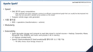
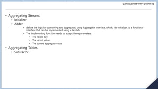
- 36. Spark및Kafka를이용한빅데이터실시간처리기술 Spark & RDD? • RDD • Spark 에서의 기본형 • 특징 • Dependencies • Partitions (with some locality information) • Compute function: Partition => Iterator[T] • 단, original model에서의 문제 • (i) compute function is opaque to Spark. Spark only sees it as a lambda expression. • (ii) Iterator[T] data type is also opaque for Python RDDs. • (iii) Spark has no way to optimize the expression • (iv) Spark has no knowledge of specific data type in T.
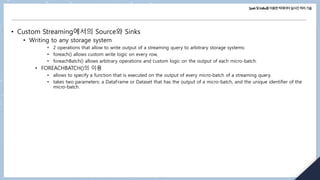
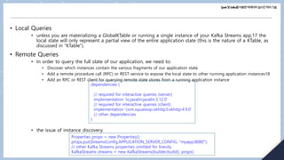
- 37. Spark및Kafka를이용한빅데이터실시간처리기술 Structuring Spark • 장점 • Low-level RDD API vs. high-level DSL # In Python # Create an RDD of tuples (name, age) dataRDD = sc.parallelize([("Brooke", 20), ("Denny", 31), ("Jules", 30), ("TD", 35), ("Brooke", 25)]) # Use map and reduceByKey transformations with lambda # expressions to aggregate and then compute average agesRDD = (dataRDD .map(lambda x: (x[0], (x[1], 1))) .reduceByKey(lambda x, y: (x[0] + y[0], x[1] + y[1])) .map(lambda x: (x[0], x[1][0]/x[1][1]))) # In Python from pyspark.sql import SparkSession from pyspark.sql.functions import avg # Create a DataFrame using SparkSession spark = (SparkSession .builder .appName("AuthorsAges") .getOrCreate()) # Create a DataFrame data_df = spark.createDataFrame([("Brooke", 20), ("Denny", 31), ("Jules", 30), ("TD", 35), ("Brooke", 25)], ["name", "age"]) # Group the same names together, aggregate, and average avg_df = data_df.groupBy("name").agg(avg("age")) # Show the results of the final execution avg_df.show() +------+--------+ | name|avg(age)| +------+--------+ |Brooke| 22.5| | Jules| 30.0| | TD| 35.0| | Denny| 31.0| +------+--------+
- 38. Spark및Kafka를이용한빅데이터실시간처리기술 // In Scala import org.apache.spark.sql.functions.avg import org.apache.spark.sql.SparkSession // Create a DataFrame using SparkSession val spark = SparkSession .builder .appName("AuthorsAges") .getOrCreate() // Create a DataFrame of names and ages val dataDF = spark.createDataFrame(Seq(("Brooke", 20), ("Brooke", 25), ("Denny", 31), ("Jules", 30), ("TD", 35))).toDF("name", "age") // Group the same names together, aggregate their ages, and compute an average val avgDF = dataDF.groupBy("name").agg(avg("age")) // Show the results of the final execution avgDF.show() +------+--------+ | name|avg(age)| +------+--------+ |Brooke| 22.5| | Jules| 30.0| | TD| 35.0| | Denny| 31.0| +------+--------+
- 39. Spark및Kafka를이용한빅데이터실시간처리기술 DataFrame API • Spark의 Basic Data Types • Spark의 Structured and Complex Data Types • Schema • schema-on-read 의 장점 • DataFrame 생성 $SPARK_HOME/bin/spark-shell scala> import org.apache.spark.sql.types._ import org.apache.spark.sql.types._ scala> val nameTypes = StringType nameTypes: org.apache.spark.sql.types.StringType.type = StringType scala> val firstName = nameTypes firstName: org.apache.spark.sql.types.StringType.type = StringType scala> val lastName = nameTypes lastName: org.apache.spark.sql.types.StringType.type = StringType
- 40. Spark및Kafka를이용한빅데이터실시간처리기술 Spark에서의 Basic Scala data types Data type Value assigned in Scala API to instantiate ByteType Byte DataTypes.ByteType ShortType Short DataTypes.ShortType IntegerType Int DataTypes.IntegerType LongType Long DataTypes.LongType FloatType Float DataTypes.FloatType DoubleType Double DataTypes.DoubleType StringType String DataTypes.StringType BooleanType Boolean DataTypes.BooleanType DecimalType java.math.BigDecimal DecimalType
- 41. Spark및Kafka를이용한빅데이터실시간처리기술 Spark에서의 Basic Python data types Data type Value assigned in Python API to instantiate ByteType int DataTypes.ByteType ShortType int DataTypes.ShortType IntegerType int DataTypes.IntegerType LongType int DataTypes.LongType FloatType float DataTypes.FloatType DoubleType Float DataTypes.DoubleType StringType str DataTypes.StringType BooleanType bool DataTypes.BooleanType DecimalType decimal.Decimal DecimalType
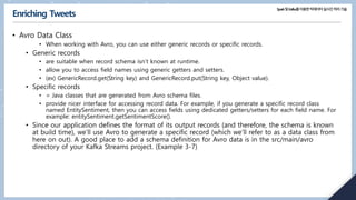
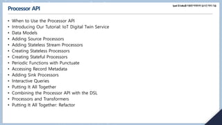
- 42. Spark및Kafka를이용한빅데이터실시간처리기술 • Spark’s Structured and Complex Data Types Spark에서의 Scala structured data types Data type Value assigned in Scala API to instantiate BinaryType Array[Byte] DataTypes.BinaryType TimestampType java.sql.Timestamp DataTypes.TimestampType DateType java.sql.Date DataTypes.DateType ArrayType scala.collection.Seq DataTypes.createArrayType(ElementTy pe) MapType scala.collection.Map DataTypes.createMapType(keyType, valueType) StructType org.apache.spark.sql.Row StructType(ArrayType[fieldTypes]) StructField A value type corresponding to the type of this field StructField(name, dataType, [nullable])
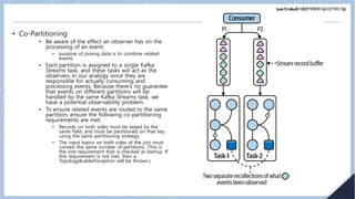
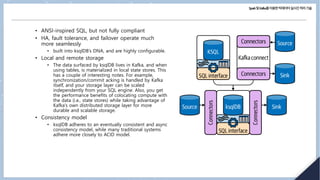
- 43. Spark및Kafka를이용한빅데이터실시간처리기술 Spark에서의 Python structured data types Data type Value assigned in Python API to instantiate BinaryType Bytearray BinaryType() TimestampType datetime.datetime TimestampType() DateType datetime.date DateType() ArrayType List, tuple, or array ArrayType(dataType, [nullable]) MapType Dict MapType(keyType, valueType, [nullable]) StructType List or tuple StructType([fields]) StructField A value type corresponding to the type of this field StructField(name, dataType, [nullable])
- 44. Spark및Kafka를이용한빅데이터실시간처리기술 • Schema 지정의 2가지 방법 • (i) 프로그램에 의한 DataFrame 용의 schema 생성: • (ii) DDL의 이용(simpler): // In Scala import org.apache.spark.sql.types._ val schema = StructType(Array(StructField("author", StringType, false), StructField("title", StringType, false), StructField("pages", IntegerType, false))) # In Python from pyspark.sql.types import * schema = StructType([StructField("author", StringType(), False), StructField("title", StringType(), False), StructField("pages", IntegerType(), False)]) // In Scala val schema = "author STRING, title STRING, pages INT" # In Python schema = "author STRING, title STRING, pages INT" # In Python from pyspark.sql import SparkSession
- 45. // In Scala val schema = "author STRING, title STRING, pages INT" # In Python schema = "author STRING, title STRING, pages INT" # In Python from pyspark.sql import SparkSession # Define schema for our data using DDL schema = "`Id` INT, `First` STRING, `Last` STRING, `Url` STRING, `Published` STRING, `Hits` INT, `Campaigns` ARRAY<STRING>" # Create our static data data = [[1, "Jules", "Damji", "https://tinyurl.1", "1/4/2016", 4535, ["twitter", "LinkedIn"]], [2, "Brooke","Wenig", "https://tinyurl.2", "5/5/2018", 8908, ["twitter", "LinkedIn"]], [3, "Denny", "Lee", "https://tinyurl.3", "6/7/2019", 7659, ["web", "twitter", "FB", "LinkedIn"]], [4, "Tathagata", "Das", "https://tinyurl.4", "5/12/2018", 10568, ["twitter", "FB"]], [5, "Matei","Zaharia", "https://tinyurl.5", "5/14/2014", 40578, ["web", "twitter", "FB", "LinkedIn"]], [6, "Reynold", "Xin", "https://tinyurl.6", "3/2/2015", 25568, ["twitter", "LinkedIn"]] ] if __name__ == "__main__": spark = (SparkSession .builder .appName("Example-3_6") .getOrCreate()) # Create a DataFrame using the schema defined above blogs_df = spark.createDataFrame(data, schema) # Show the DataFrame; it should reflect our table above blogs_df.show() # Print the schema used by Spark to process the DataFrame print(blogs_df.printSchema())
- 46. Spark및Kafka를이용한빅데이터실시간처리기술 • to read data from a JSON file // In Scala package main.scala.chapter3 import org.apache.spark.sql.SparkSession import org.apache.spark.sql.types._ object Example3_7 { def main(args: Array[String]) { val spark = SparkSession .builder .appName("Example-3_7") .getOrCreate() if (args.length <= 0) { println("usage Example3_7 <file path to blogs.json>") System.exit(1) } val jsonFile = args(0) // Get the path to the JSON file // Define our schema programmatically val schema = StructType(Array(StructField("Id", IntegerType, false), StructField("First", StringType, false), StructField("Last", StringType, false), StructField("Url", StringType, false), StructField("Published", StringType, false),
- 47. Spark및Kafka를이용한빅데이터실시간처리기술 • Column과 Expression 이용 // In Scala scala> import org.apache.spark.sql.functions._ scala> blogsDF.columns res2: Array[String] = Array(Campaigns, First, Hits, Id, Last, Published, Url) // Access a particular column with col and it returns a Column type scala> blogsDF.col("Id") res3: org.apache.spark.sql.Column = id // Use an expression to compute a value scala> blogsDF.select(expr("Hits * 2")).show(2) // or use col to compute value scala> blogsDF.select(col("Hits") * 2).show(2) +----------+ |(Hits * 2)| +----------+ | 9070| | 17816| +----------+
- 48. Spark및Kafka를이용한빅데이터실시간처리기술 // Use an expression to compute big hitters for blogs // This adds a new column, Big Hitters, based on the conditional expression blogsDF.withColumn("Big Hitters", (expr("Hits > 10000"))).show() +---+---------+-------+---+---------+-----+-----------------+-----------+ | Id| First| Last|Url|Published| Hits| Campaigns|Big Hitters| +---+---------+-------+---+---------+-----+-----------------+-----------+ | 1| Jules| Damji|...| 1/4/2016| 4535| [twitter, LinkedIn]| false| | 2| Brooke| Wenig|...| 5/5/2018| 8908| [twitter, LinkedIn]| false| | 3| Denny| Lee|...| 6/7/2019| 7659|[web, twitter, FB...| false| | 4|Tathagata| Das|...|5/12/2018|10568| [twitter, FB]| true| | 5| Matei|Zaharia|...|5/14/2014|40578|[web, twitter, FB...| true| | 6| Reynold| Xin|...| 3/2/2015|25568| [twitter, LinkedIn]| true| +---+---------+-------+---+---------+-----+-----------------+-----------+
- 49. Spark및Kafka를이용한빅데이터실시간처리기술 // Concatenate three columns, create a new column, and show the // newly created concatenated column blogsDF .withColumn("AuthorsId", (concat(expr("First"), expr("Last"), expr("Id")))) .select(col("AuthorsId")) .show(4) +-------------+ | AuthorsId| +-------------+ | JulesDamji1| | BrookeWenig2| | DennyLee3| |TathagataDas4| +-------------+ // These statements return the same value, showing that // expr is the same as a col method call blogsDF.select(expr("Hits")).show(2) blogsDF.select(col("Hits")).show(2) blogsDF.select("Hits").show(2) +-----+ | Hits| +-----+ | 4535| | 8908| +-----+
- 50. Spark및Kafka를이용한빅데이터실시간처리기술 // Sort by column "Id" in descending order blogsDF.sort(col("Id").desc).show() blogsDF.sort($"Id".desc).show() +-----------------+---------+-----+---+-------+---------+--------------+ | Campaigns| First| Hits| Id| Last|Published| Url| +-----------------+---------+-----+---+-------+---------+--------------+ | [twitter, LinkedIn]| Reynold|25568| 6| Xin| 3/2/2015|https://tinyurl.6| |[web, twitter, FB...| Matei|40578| 5|Zaharia|5/14/2014|https://tinyurl.5| | [twitter, FB]|Tathagata|10568| 4| Das|5/12/2018|https://tinyurl.4| |[web, twitter, FB...| Denny| 7659| 3| Lee| 6/7/2019|https://tinyurl.3| | [twitter, LinkedIn]| Brooke| 8908| 2| Wenig| 5/5/2018|https://tinyurl.2| | [twitter, LinkedIn]| Jules| 4535| 1| Damji| 1/4/2016|https://tinyurl.1| +-----------------+---------+-----+---+-------+---------+--------------+
- 51. Spark및Kafka를이용한빅데이터실시간처리기술 • Rows // In Scala import org.apache.spark.sql.Row // Create a Row val blogRow = Row(6, "Reynold", "Xin", "https://tinyurl.6", 255568, "3/2/2015", Array("twitter", "LinkedIn")) // Access using index for individual items blogRow(1) res62: Any = Reynold # In Python from pyspark.sql import Row blog_row = Row(6, "Reynold", "Xin", "https://tinyurl.6", 255568, "3/2/2015", ["twitter", "LinkedIn"]) # access using index for individual items blog_row[1] 'Reynold’ # Row objects can be used to create DFs if you need quick interactivity and exploration: # In Python rows = [Row("Matei Zaharia", "CA"), Row("Reynold Xin", "CA")] authors_df = spark.createDataFrame(rows, ["Authors", "State"]) authors_df.show() // In Scala val rows = Seq(("Matei Zaharia", "CA"), ("Reynold Xin", "CA")) val authorsDF = rows.toDF("Author", "State") authorsDF.show() +-------------+-----+ | Author|State| +-------------+-----+ |Matei Zaharia| CA| | Reynold Xin| CA| +-------------+-----+
- 52. Spark및Kafka를이용한빅데이터실시간처리기술 • 일반적인 DataFrame Operations • DataFrameReader와 DataFrameWriter • SAVING A DATAFRAME AS A PARQUET FILE OR SQL TABLE • ((code)) • Transformation과 actions • PROJECTION과 FILTER • projection • = returns only the rows matching a certain condition using filters. • projections with select() method, while filters using filter() or where(). • Column의 rename, add, drop • Aggregation • 기타의 일반적인 DataFrame operations • ((code))
- 53. Spark및Kafka를이용한빅데이터실시간처리기술 Dataset API • Spark 2.0의 unified DataFrame과 Dataset APIs as Structured APIs • DataFrame = an alias for a collection of generic objects, Dataset[Row], where a Row is a generic untyped JVM object that may hold different types of fields. • Dataset = a collection of strongly typed JVM objects in Scala or a class in Java. • = a strongly typed collection of domain-specific objects that can be transformed in parallel using functional or relational operations. • Each Dataset [in Scala] also has an untyped view called a DataFrame, which is a Dataset of Row.
- 54. Spark및Kafka를이용한빅데이터실시간처리기술 • Typed Objects, Untyped Objects, and Generic Rows • Spark에서의 Typed 및 untyped objects • Internally, Spark manipulates Row objects, converting them to equivalent types. • Dataset의 생성 • Dataset Operations Language Typed 및 untyped main abstraction Typed or untyped Scala Dataset[T] 와 DataFrame (alias for Dataset[Row]) Both typed and untyped Java Dataset<T> Typed Python DataFrame Generic Row untyped R DataFrame Generic Row untyped
- 55. Spark및Kafka를이용한빅데이터실시간처리기술 DataFrames vs. Datasets • 일반사항 • 예 • … • When to Use RDDs • Are using a third-party package that’s written using RDDs • Can forgo the code optimization, efficient space utilization, and performance benefits available with DataFrames and Datasets • Want to precisely instruct Spark how to do a query
- 56. Spark및Kafka를이용한빅데이터실시간처리기술 Spark SQL (Preview) • (Spark SQL과 엔진)
- 57. Spark및Kafka를이용한빅데이터실시간처리기술 • Catalyst Optimizer • Phase 1: Analysis • Phase 2: Logical optimization • Phase 3: Physical planning • Phase 4: Code generation • ((code: M&Ms example))
- 58. Spark및Kafka를이용한빅데이터실시간처리기술 Spark SQL과 DataFrames • Spark SQL의 이용 • SQL Table과 View • Managed vs. UnmanagedTables • SQL Database와 Table의 생성 • View 생성 • Viewing the Metadata • Caching SQL Tables • Reading Tables into DataFrames • DataFrame과 SQL Tables의 데이터 소스 • DataFrameReader와 DataFrameWriter • Parquet • JSON, CSV • Avro • ORC • Image와 Binary Files
- 60. Spark및Kafka를이용한빅데이터실시간처리기술 Spark SQL의 이용 • Query 예 // In Scala import org.apache.spark.sql.SparkSession val spark = SparkSession .builder .appName("SparkSQLExampleApp") .getOrCreate() // Path to data set val csvFile="/databricks-datasets/learning-spark-v2/flights/departuredelays.csv" // Read and create a temporary view // Infer schema (note that for larger files you may want to specify the schema) val df = spark.read.format("csv") .option("inferSchema", "true") .option("header", "true") .load(csvFile) // Create a temporary view df.createOrReplaceTempView("us_delay_flights_tbl")
- 61. Spark및Kafka를이용한빅데이터실시간처리기술 • To specify a schema, use a DDL-formatted string. # In Python from pyspark.sql import SparkSession # Create a SparkSession spark = (SparkSession .builder .appName("SparkSQLExampleApp") .getOrCreate()) # Path to data set csv_file = "/databricks-datasets/learning-spark-v2/flights/departuredelays.csv" # Read and create a temporary view # Infer schema (note that for larger files you # may want to specify the schema) df = (spark.read.format("csv") .option("inferSchema", "true") .option("header", "true") .load(csv_file)) df.createOrReplaceTempView("us_delay_flights_tbl") // In Scala val schema = "date STRING, delay INT, distance INT, origin STRING, destination STRING“ # In Python schema = "`date` STRING, `delay` INT, `distance` INT, `origin` STRING, `destination` STRING"
- 62. Spark및Kafka를이용한빅데이터실시간처리기술 SQL Table과 View • Managed vs. Unmanaged Tables • managed table ; Spark manages both metadata and data. (a local filesystem, HDFS, or an object store). • unmanaged table, Spark only manages metadata, while you manage data yourself in an external data source (ex: Cassandra). • SQL Database와 Table 생성 • managed table의 생성 // In Scala/Python spark.sql("CREATE DATABASE learn_spark_db") spark.sql("USE learn_spark_db") // In Scala/Python spark.sql("CREATE TABLE managed_us_delay_flights_tbl (date STRING, delay INT, distance INT, origin STRING, destination STRING)") # You can do the same thing using the DataFrame API like this: # In Python # Path to our US flight delays CSV file csv_file = "/databricks-datasets/learning-spark-v2/flights/departuredelays.csv" # Schema as defined in the preceding example schema="date STRING, delay INT, distance INT, origin STRING, destination STRING" flights_df = spark.read.csv(csv_file, schema=schema) flights_df.write.saveAsTable("managed_us_delay_flights_tbl")
- 63. Spark및Kafka를이용한빅데이터실시간처리기술 • unmanaged table의 생성 • View의 생성 • Temporary views vs. global temporary views • A temporary view is tied to a single SparkSession within a Spark application. • A global temporary view is visible across multiple SparkSessions within a Spark application. • application 내에서 여러 개의 SparkSession을 생성할 수 있음 • 예: in cases where you want to access (and combine) data from two different SparkSessions that don’t share the same Hive metastore configurations. # To create an unmanaged table from a data source such as a CSV file, in SQL use: spark.sql("""CREATE TABLE us_delay_flights_tbl(date STRING, delay INT, distance INT, origin STRING, destination STRING) USING csv OPTIONS (PATH '/databricks-datasets/learning-spark-v2/flights/departuredelays.csv')""") # And within the DataFrame API use: (flights_df .write .option("path", "/tmp/data/us_flights_delay") .saveAsTable("us_delay_flights_tbl"))
- 64. Spark및Kafka를이용한빅데이터실시간처리기술 • Viewing Metadata • Caching SQL Tables • Table을 DataFrame에 읽어 들이기 // In Scala/Python spark.catalog.listDatabases() spark.catalog.listTables() spark.catalog.listColumns("us_delay_flights_tbl") -- In SQL CACHE [LAZY] TABLE <table-name> UNCACHE TABLE <table-name> // In Scala val usFlightsDF = spark.sql("SELECT * FROM us_delay_flights_tbl") val usFlightsDF2 = spark.table("us_delay_flights_tbl") # In Python us_flights_df = spark.sql("SELECT * FROM us_delay_flights_tbl") us_flights_df2 = spark.table("us_delay_flights_tbl")
- 65. Spark및Kafka를이용한빅데이터실시간처리기술 DataFrame과 SQL Tables의 데이터 소스 • DataFrameReader • DataFrameReader methods, arguments, and options Method Arguments Description format() "parquet", "csv", "txt", "json", "jdbc", "orc", "avro", etc. default is Parquet or whatever is set in spark.sql.sources.default. option() ("mode", {PERMISSIVE | FAILFAST | DROPMALFORMED } ) ("inferSchema", {true | false}) ("path", "path_file_data_source") A series of key/value pairs and options. Default: PERMISSIVE. "inferSchema" and "mode" options are specific to JSON and CSV file formats. schema() DDL String or StructType 예: 'A INT, B STRING’ or StructType(...) JSON or CSV format의 경우 option() method에서 infer schema 지정 가능. load() "/path/to/data/source" path to data source.
- 66. Spark및Kafka를이용한빅데이터실시간처리기술 • DataFrameWriter • DataFrameWriter methods, arguments, and options Method Arguments Description format() "parquet", "csv", "txt", "json", "jdbc", "orc", "avro", etc. default is Parquet or whatever set in spark.sql.sources.default. option() ("mode", {append | overwrite | ignore | error or errorifexists} ) ("mode", {SaveMode.Overwrite | SaveMode.Append, SaveMode.Ignore, SaveMode.ErrorIfExists}) ("path", "path_to_write_to") A series of key/value pairs and options. This is an overloaded method. The default mode options are error or errorifexists and SaveMode.ErrorIfExists; they throw an exception at runtime if the data already exists. bucketBy() (numBuckets, col, col..., coln) number of buckets and names of columns to bucket by. Uses Hive’s bucketing scheme on a filesystem. save() "/path/to/data/source" The path to save to. saveAsTable() "table_name" The table to save to.
- 67. Spark및Kafka를이용한빅데이터실시간처리기술 // In Scala // Use Parquet val file = """/databricks-datasets/learning-spark-v2/flights/summary- data/parquet/2010-summary.parquet""" val df = spark.read.format("parquet").load(file) // Use Parquet; you can omit format("parquet") if you wish as it's the default val df2 = spark.read.load(file) // Use CSV val df3 = spark.read.format("csv") .option("inferSchema", "true") .option("header", "true") .option("mode", "PERMISSIVE") .load("/databricks-datasets/learning-spark-v2/flights/summary-data/csv/*") // Use JSON val df4 = spark.read.format("json") .load("/databricks-datasets/learning-spark-v2/flights/summary-data/json/*")
- 68. Spark및Kafka를이용한빅데이터실시간처리기술 • Parquet • Parquet 파일을 DataFrame에 읽어 들이기 • Parquet 파일을 Spark SQL table 에 읽어 들이기 • Writing DataFrames to Parquet files • Writing DataFrames to Spark SQL tables • ((code))
- 69. Spark및Kafka를이용한빅데이터실시간처리기술 • JSON • JSON 파일을 DataFrame에 읽어 들이기 • JSON 파일을 Spark SQL table 에 읽어 들이기 • Writing DataFrames to JSON files • JSON data source options • JSON options for DataFrameReader and DataFrameWriter Property 이름 Values 의미 Scope compression none, uncompressed, bzip2, deflate, gzip, lz4, or snappy read will only detect the compression or codec from the file extension. Write dateFormat yyyy-MM-dd or DateTimeFormatter Use this format or any format from Java’s DateTimeFormatter. Read/write multiLine true, false Default is false (single-line mode). Read allowUnquotedFieldName s true, false Allow unquoted JSON field names. Default is false. Read
- 70. Spark및Kafka를이용한빅데이터실시간처리기술 • CSV • Reading a CSV file into a DataFrame • Reading a CSV file into a Spark SQL table • Writing DataFrames to CSV files • CSV data source options • Avro • Reading an Avro file into a DataFrame • Reading an Avro file into a Spark SQL table • Writing DataFrames to Avro files • Avro data source options
- 71. Spark및Kafka를이용한빅데이터실시간처리기술 • ORC • Reading an ORC file into a DataFrame • Reading an ORC file into a Spark SQL table • Writing DataFrames to ORC files • Images • Reading an image file into a DataFrame • Binary Files • eading a binary file into a DataFrame
- 72. Spark및Kafka를이용한빅데이터실시간처리기술 Spark SQL (1) – Spark SQL & DataFrame
- 73. Spark및Kafka를이용한빅데이터실시간처리기술 Spark SQL과 DataFrames • Spark SQL과 Apache Hive • User-Defined Functions • Spark SQL Shell, Beeline를 이용한 Query • External Data Sources • JDBC 및 SQL Databases • 기타의 External Sources • DataFrame과 Spark SQL에서의 Higher-Order Functions • Option 1: Explode와 Collect • Option 2: User-Defined Function • Complex Data Type을 위한 내장 함수 • Higher-Order Functions • 일반적인 DataFrames과 Spark SQL의 Operations • Unions, Joins, Windowing, Modifications
- 74. Spark및Kafka를이용한빅데이터실시간처리기술 Spark SQL과 Apache Hive • User-Defined Functions • Spark SQL UDFs // In Scala // Create cubed function val cubed = (s: Long) => { s * s * s } // Register UDF spark.udf.register("cubed", cubed) // Create temporary view spark.range(1, 9).createOrReplaceTempView("udf_test") # In Python from pyspark.sql.types import LongType # Create cubed function def cubed(s): return s * s * s # Register UDF spark.udf.register("cubed", cubed, LongType()) # Generate temporary view spark.range(1, 9).createOrReplaceTempView("udf_test")
- 75. Spark및Kafka를이용한빅데이터실시간처리기술 // In Scala/Python // Query the cubed UDF spark.sql("SELECT id, cubed(id) AS id_cubed FROM udf_test").show() +---+--------+ | id|id_cubed| +---+--------+ | 1| 1| | 2| 8| | 3| 27| | 4| 64| | 5| 125| | 6| 216| | 7| 343| | 8| 512| +---+--------+
- 76. Spark및Kafka를이용한빅데이터실시간처리기술 • Pandas UDFs를 이용한 PySpark UDFs 배포에서의 속도 개선 • Issues: PySpark UDFs are slower than Scala UDFs. • Solution: Pandas UDFs (= vectorized UDFs) in Spark 2.3. • 특히 Spark 3.0 + > Python 3.6에서 Pandas UDF는 다음 2개로 분리 • Pandas UDFs • Pandas UDFs infer the Pandas UDF type from Python type hints in Pandas UDFs (예: pandas.Series, pandas.DataFrame, Tuple, and Iterator) (Spark 3.0) • 기존: 각 Pandas UDF type을 manually define and specify. • 지원되는 Python type hints in Pandas UDFs: Series to Series, Iterator of Series to Iterator of Series, Iterator of Multiple Series to Iterator of Series, and Series to Scalar (a single value). • Pandas Function APIs • allow to directly apply a local Python function to a PySpark DataFrame where both the input and output are Pandas instances. For Spark 3.0, the supported Pandas Function APIs are grouped map, map, co-grouped map.
- 77. Spark및Kafka를이용한빅데이터실시간처리기술 Spark SQL Shell, Beeline를 이용한 Query • Spark SQL Shell의 이용 • (…) • While communicating with Hive metastore service in local mode, it does not talk to Thrift JDBC/ODBC server (a.k.a. Spark Thrift Server or STS). • STS allows JDBC/ODBC clients to execute SQL queries over JDBC and ODBC protocols on Apache Spark. • To start Spark SQL CLI: ./bin/spark-sql • Create a table spark-sql> CREATE TABLE people (name STRING, age int); • Insert data into the table INSERT INTO people SELECT name, age FROM ... spark-sql> INSERT INTO people VALUES ("Michael", NULL); Time taken: 1.696 seconds • Running a Spark SQL query spark-sql> SHOW TABLES; spark-sql> SELECT * FROM people WHERE age < 20;
- 78. Spark및Kafka를이용한빅데이터실시간처리기술 • Beeline의 이용 • (…) • Beeline is a JDBC client based on SQLLine CLI. • You can use this to execute Spark SQL queries against the Spark Thrift server. • Start the Thrift server ./sbin/start-thriftserver.sh ./sbin/start-all.sh • Connect to the Thrift server via Beeline ./bin/beeline !connect jdbc:hive2://localhost:10000 • Execute a Spark SQL query with Beeline 0: jdbc:hive2://localhost:10000> SHOW tables; • Stop the Thrift server ./sbin/stop-thriftserver.sh
- 79. Spark및Kafka를이용한빅데이터실시간처리기술 External Data Sources • JDBC와 SQL Databases • specify JDBC driver for JDBC data source and make on the Spark classpath. ./bin/spark-shell --driver-class-path $database.jar --jars $database.jar Property name Description user, password These are normally provided as connection properties for logging into the data sources. url JDBC connection URL, e.g., jdbc:postgresql://localhost/test?user=fred&password=secret. dbtable JDBC table to read from or write to. You can’t specify the dbtable and query options at the same time. query Query to be used to read data from Apache Spark, e.g., SELECT column1, column2, ..., columnN FROM [table|subquery]. You can’t specify the query and dbtable options at the same time. driver Class name of the JDBC driver to use to connect to the specified URL.
- 80. Spark및Kafka를이용한빅데이터실시간처리기술 • Partitioning의 중요성 • Spark SQL와 외부의 JDBC source와 대량 데이터 전달 시 partition the data source! Property name Description numPartitions The maximum number of partitions that can be used for parallelism in table reading and writing. This also determines the maximum number of concurrent JDBC connections. partitionColumn When reading an external source, partitionColumn is the column that is used to determine the partitions; note, partitionColumn must be a numeric, date, or timestamp column. lowerBound Sets the minimum value of partitionColumn for the partition stride. upperBound Sets the maximum value of partitionColumn for the partition stride. numPartitions: 10 lowerBound: 1000 upperBound: 10000 SELECT * FROM table WHERE partitionColumn BETWEEN 1000 and 2000 SELECT * FROM table WHERE partitionColumn BETWEEN 2000 and 3000 ... SELECT * FROM table WHERE partitionColumn BETWEEN 9000 and 10000
- 81. Spark및Kafka를이용한빅데이터실시간처리기술 기타의 External Sources • PostgreSQL • MySQL • Azure Cosmos DB • MS SQL Server
- 82. Spark및Kafka를이용한빅데이터실시간처리기술 DataFrame과 Spark SQL에서의 Higher-Order Functions • 2 typical solutions for manipulating complex data types • Nested structure를 개별 row로 explode → apply function → re-create nested structure • (ii) Build a user-defined function such as get_json_object(), from_json(), to_json(), explode(), and selectExpr(). • Option 1: Explode and Collect • Option 2: User-Defined Function • then use this UDF in Spark SQL: spark.sql("SELECT id, plusOneInt(values) AS values FROM table").show() • serialization and deserialization process itself may be expensive. However collect_list() may cause executors to experience out-of-memory issues for large data sets, whereas using UDFs would alleviate these issues. -- In SQL SELECT id, collect_list(value + 1) AS values FROM (SELECT id, EXPLODE(values) AS value FROM table) x GROUP BY id // In Scala def addOne(values: Seq[Int]): Seq[Int] = { values.map(value => value + 1) } val plusOneInt = spark.udf.register("plusOneInt", addOne(_: Seq[Int]): Seq[Int])
- 83. Spark및Kafka를이용한빅데이터실시간처리기술 Complex Data Type을 위한 내장 함수 • Complex Data Type에 대한 내장 함수 • Array type functions Function/Description Query Output array_distinct(array<T>): array<T> SELECT array_distinct(array(1, 2, 3, null, 3)); [1,2,3,null] array_intersect(array<T>, array<T>): array<T> SELECT array_intersect(array(1, 2, 3), array(1, 3, 5)); [1,3] array_union(array<T>, array<T>): array<T> SELECT array_union(array(1, 2, 3), array(1, 3, 5)); [1,2,3,5] array_except(array<T>, array<T>): array<T> SELECT array_except(array(1, 2, 3), array(1, 3, 5)); [2] array_join(array<String>, String[, String]): String SELECT array_join(array('hello', 'world'), ' '); hello world
- 84. Spark및Kafka를이용한빅데이터실시간처리기술 • Complex Data Type을 위한 내장 함수 • Map functions Function/Description Query Output map_form_arrays(array<K>, array<V>): map<K, V> SELECT map_from_arrays(array(1.0, 3.0), array('2', '4')); {"1.0":"2", "3.0":"4"} map_from_entries(array<struct<K, V>>): map<K, V> SELECT map_from_entries(array(struct(1, 'a'), struct(2, 'b'))); {"1":"a", "2":"b"} map_concat(map<K, V>, ...): map<K, V> SELECT map_concat(map(1, 'a', 2, 'b'), map(2, 'c', 3, 'd')); {"1":"a", "2":"c","3":"d"} element_at(map<K, V>, K): V SELECT element_at(map(1, 'a', 2, 'b'), 2); B cardinality(array<T>): Int SELECT cardinality(map(1, 'a', 2, 'b')); 2
- 85. Spark및Kafka를이용한빅데이터실시간처리기술 • Higher-Order Functions • (…) • 내장함수 외에도: higher-order functions • 예: -- In SQL transform(values, value -> lambda expression) # In Python from pyspark.sql.types import * schema = StructType([StructField("celsius", ArrayType(IntegerType()))]) t_list = [[35, 36, 32, 30, 40, 42, 38]], [[31, 32, 34, 55, 56]] t_c = spark.createDataFrame(t_list, schema) t_c.createOrReplaceTempView("tC") # Show the DataFrame t_c.show() // In Scala // Create DataFrame with two rows of two arrays (tempc1, tempc2) val t1 = Array(35, 36, 32, 30, 40, 42, 38) val t2 = Array(31, 32, 34, 55, 56) val tC = Seq(t1, t2).toDF("celsius") tC.createOrReplaceTempView("tC") // Show the DataFrame tC.show() +--------------------+ | celsius| +--------------------+ |[35, 36, 32, 30, ...| |[31, 32, 34, 55, 56]| +--------------------+
- 86. Spark및Kafka를이용한빅데이터실시간처리기술 • transform() • transform(array<T>, function<T, U>): array<U> • filter() filter(array<T>, function<T, Boolean>): array<T> // In Scala/Python // Calculate Fahrenheit from Celsius for an array of temperatures spark.sql(""" SELECT celsius, transform(celsius, t -> ((t * 9) div 5) + 32) as fahrenheit FROM tC """).show() +--------------------+--------------------+ | celsius| fahrenheit| +--------------------+--------------------+ |[35, 36, 32, 30, ...|[95, 96, 89, 86, ...| |[31, 32, 34, 55, 56]|[87, 89, 93, 131,...| +--------------------+--------------------+ // In Scala/Python // Filter temperatures > 38C for array of temperatures spark.sql(""" SELECT celsius, filter(celsius, t -> t > 38) as high FROM tC """).show() +--------------------+--------+ | celsius| high| +--------------------+--------+ |[35, 36, 32, 30, ...|[40, 42]| |[31, 32, 34, 55, 56]|[55, 56]| +--------------------+--------+
- 87. Spark및Kafka를이용한빅데이터실시간처리기술 • exists() exists(array<T>, function<T, V, Boolean>): Boolean • reduce() reduce(array<T>, B, function<B, T, B>, function<B, R>) // In Scala/Python // Is there a temperature of 38C in the array of temperatures spark.sql(""" SELECT celsius, exists(celsius, t -> t = 38) as threshold FROM tC """).show() +--------------------+---------+ | celsius|threshold| +--------------------+---------+ |[35, 36, 32, 30, ...| true| |[31, 32, 34, 55, 56]| false| +--------------------+---------+ // In Scala/Python // Calculate average temperature and convert to F spark.sql(""" SELECT celsius, reduce( celsius, 0, (t, acc) -> t + acc, acc -> (acc div size(celsius) * 9 div 5) + 32 ) as avgFahrenheit FROM tC """).show() +--------------------+-------------+ | celsius|avgFahrenheit| +--------------------+-------------+ |[35, 36, 32, 30, ...| 96| |[31, 32, 34, 55, 56]| 105| +--------------------+-------------+
- 88. Spark및Kafka를이용한빅데이터실시간처리기술 일반적인 DataFrames과 Spark SQL의 Operations • (…) • Aggregate 함수 • Collection 함수 • Datetime 함수 • Math 함수 • Miscellaneous 함수 • Non-aggregate 함수 • Sorting 함수 • String 함수 • UDF 함수 • Window 함수 • For full list, see Spark SQL documentation. • 코드 실습을 위한 데이터 생성 ((code))
- 89. Spark및Kafka를이용한빅데이터실시간처리기술 // In Scala import org.apache.spark.sql.functions._ // Set file paths val delaysPath = "/databricks-datasets/learning-spark-v2/flights/departuredelays.csv" val airportsPath = "/databricks-datasets/learning-spark-v2/flights/airport-codes-na.txt" // Obtain airports data set val airports = spark.read .option("header", "true") .option("inferschema", "true") .option("delimiter", "t") .csv(airportsPath) airports.createOrReplaceTempView("airports_na") // Obtain departure Delays data set val delays = spark.read .option("header","true") .csv(delaysPath) .withColumn("delay", expr("CAST(delay as INT) as delay")) .withColumn("distance", expr("CAST(distance as INT) as distance")) delays.createOrReplaceTempView("departureDelays") // Create temporary small table val foo = delays.filter( expr("""origin == 'SEA' AND destination == 'SFO' AND date like '01010%' AND delay > 0""")) foo.createOrReplaceTempView("foo")
- 90. Spark및Kafka를이용한빅데이터실시간처리기술 # In Python # Set file paths from pyspark.sql.functions import expr tripdelaysFilePath = "/databricks-datasets/learning-spark-v2/flights/departuredelays.csv" airportsnaFilePath = "/databricks-datasets/learning-spark-v2/flights/airport-codes-na.txt" # Obtain airports data set airportsna = (spark.read .format("csv") .options(header="true", inferSchema="true", sep="t") .load(airportsnaFilePath)) airportsna.createOrReplaceTempView("airports_na") # Obtain departure delays data set departureDelays = (spark.read .format("csv") .options(header="true") .load(tripdelaysFilePath)) departureDelays = (departureDelays .withColumn("delay", expr("CAST(delay as INT) as delay")) .withColumn("distance", expr("CAST(distance as INT) as distance"))) departureDelays.createOrReplaceTempView("departureDelays") # Create temporary small table foo = (departureDelays .filter(expr("""origin == 'SEA' and destination == 'SFO' and date like '01010%' and delay > 0"""))) foo.createOrReplaceTempView("foo")
- 91. Spark및Kafka를이용한빅데이터실시간처리기술 // Scala/Python spark.sql("SELECT * FROM airports_na LIMIT 10").show() +-----------+-----+-------+----+ | City|State|Country|IATA| +-----------+-----+-------+----+ | Abbotsford| BC| Canada| YXX| | Aberdeen| SD| USA| ABR| … | Alexandria| LA| USA| AEX| | Allentown| PA| USA| ABE| +-----------+-----+-------+----+ spark.sql("SELECT * FROM departureDelays LIMIT 10").show() +--------+-----+--------+------+-----------+ | date|delay|distance|origin|destination| +--------+-----+--------+------+-----------+ |01011245| 6| 602| ABE| ATL| |01020600| -8| 369| ABE| DTW| … |01051245| 88| 602| ABE| ATL| |01050605| 9| 602| ABE| ATL| +--------+-----+--------+------+-----------+ spark.sql("SELECT * FROM foo").show() +--------+-----+--------+------+-----------+ | date|delay|distance|origin|destination| +--------+-----+--------+------+-----------+ |01010710| 31| 590| SEA| SFO| |01010955| 104| 590| SEA| SFO| |01010730| 5| 590| SEA| SFO| +--------+-----+--------+------+-----------+
- 92. Spark및Kafka를이용한빅데이터실시간처리기술 Unions, Joins, Windowing, Modifications • Unions // Scala // Union two tables val bar = delays.union(foo) bar.createOrReplaceTempView("bar") bar.filter(expr("""origin == 'SEA' AND destination == 'SFO' AND date LIKE '01010%' AND delay > 0""")).show() # In Python # Union two tables bar = departureDelays.union(foo) bar.createOrReplaceTempView("bar") # Show the union (filtering for SEA and SFO in a specific time range) bar.filter(expr("""origin == 'SEA' AND destination == 'SFO' AND date LIKE '01010%' AND delay > 0""")).show() -- In SQL spark.sql(""" SELECT * FROM bar WHERE origin = 'SEA' AND destination = 'SFO' AND date LIKE '01010%' AND delay > 0 """).show() +--------+-----+--------+------+-----------+ | date|delay|distance|origin|destination| +--------+-----+--------+------+-----------+ |01010710| 31| 590| SEA| SFO| |01010955| 104| 590| SEA| SFO| |01010730| 5| 590| SEA| SFO| |01010710| 31| 590| SEA| SFO| |01010955| 104| 590| SEA| SFO| |01010730| 5| 590| SEA| SFO| +--------+-----+--------+------+-----------+
- 93. Spark및Kafka를이용한빅데이터실시간처리기술 • Joins • Join types: inner (default), cross, outer, full, full_outer, left, left_outer, right, right_outer, left_semi, and left_anti. • More in the documentation. // In Scala foo.join( airports.as('air), $"air.IATA" === $"origin" ).select("City", "State", "date", "delay", "distance", "destination").show() # In Python # Join departure delays data (foo) with airport info foo.join( airports, airports.IATA == foo.origin ).select("City", "State", "date", "delay", "distance", "destination").show() -- In SQL spark.sql(""" SELECT a.City, a.State, f.date, f.delay, f.distance, f.destination FROM foo f JOIN airports_na a ON a.IATA = f.origin """).show() +-------+-----+--------+-----+--------+-----------+ | City|State| date|delay|distance|destination| +-------+-----+--------+-----+--------+-----------+ |Seattle| WA|01010710| 31| 590| SFO| |Seattle| WA|01010955| 104| 590| SFO| |Seattle| WA|01010730| 5| 590| SFO| +-------+-----+--------+-----+--------+-----------+
- 94. Spark및Kafka를이용한빅데이터실시간처리기술 • Windowing • uses values from the rows in a window (a range of input rows) to return a set of values, typically in the form of another row. • --> operate on a group of rows while still returning a single value for every input row. In this section, we will show how to use the dense_rank() window function; there are many other functions SQL DataFrame API Ranking functions rank() rank() dense_rank() denseRank() percent_rank() percentRank() ntile() ntile() row_number() rowNumber() Analytic functions cume_dist() cumeDist() first_value() firstValue() last_value() lastValue() lag() lag() lead() lead()
- 95. Spark및Kafka를이용한빅데이터실시간처리기술 -- In SQL DROP TABLE IF EXISTS departureDelaysWindow; CREATE TABLE departureDelaysWindow AS SELECT origin, destination, SUM(delay) AS TotalDelays FROM departureDelays WHERE origin IN ('SEA', 'SFO', 'JFK') AND destination IN ('SEA', 'SFO', 'JFK', 'DEN', 'ORD', 'LAX', 'ATL') GROUP BY origin, destination; SELECT * FROM departureDelaysWindow +------+-----------+-----------+ |origin|destination|TotalDelays| +------+-----------+-----------+ | JFK| ORD| 5608| | SEA| LAX| 9359| | JFK| SFO| 35619| | SFO| ORD| 27412| … | JFK| SEA| 7856| | JFK| LAX| 35755| | SFO| JFK| 24100| | SFO| LAX| 40798| | SEA| JFK| 4667| +------+-----------+-----------+
- 96. Spark및Kafka를이용한빅데이터실시간처리기술 • to find the three destinations that experienced the most delays • a better approach -- In SQL SELECT origin, destination, SUM(TotalDelays) AS TotalDelays FROM departureDelaysWindow WHERE origin = '[ORIGIN]' GROUP BY origin, destination ORDER BY SUM(TotalDelays) DESC LIMIT 3 -- In SQL spark.sql(""" SELECT origin, destination, TotalDelays, rank FROM ( SELECT origin, destination, TotalDelays, dense_rank() OVER (PARTITION BY origin ORDER BY TotalDelays DESC) as rank FROM departureDelaysWindow ) t WHERE rank <= 3 """).show() +------+-----------+-----------+----+ |origin|destination|TotalDelays|rank| +------+-----------+-----------+----+ | SEA| SFO| 22293| 1| | SEA| DEN| 13645| 2| | SEA| ORD| 10041| 3| | SFO| LAX| 40798| 1| | SFO| ORD| 27412| 2| | SFO| JFK| 24100| 3| | JFK| LAX| 35755| 1| | JFK| SFO| 35619| 2| | JFK| ATL| 12141| 3| +------+-----------+-----------+----+
- 97. Spark및Kafka를이용한빅데이터실시간처리기술 • Modifications • Adding new columns // In Scala/Python foo.show() --------+-----+--------+------+-----------+ | date|delay|distance|origin|destination| +--------+-----+--------+------+-----------+ |01010710| 31| 590| SEA| SFO| |01010955| 104| 590| SEA| SFO| |01010730| 5| 590| SEA| SFO| +--------+-----+--------+------+-----------+ // In Scala import org.apache.spark.sql.functions.expr val foo2 = foo.withColumn( "status", expr("CASE WHEN delay <= 10 THEN 'On-time' ELSE 'Delayed' END") ) # In Python from pyspark.sql.functions import expr foo2 = (foo.withColumn( "status", expr("CASE WHEN delay <= 10 THEN 'On-time' ELSE 'Delayed' END") )) // In Scala/Python foo2.show() +--------+-----+--------+------+-----------+-------+ | date|delay|distance|origin|destination| status| +--------+-----+--------+------+-----------+-------+ |01010710| 31| 590| SEA| SFO|Delayed| |01010955| 104| 590| SEA| SFO|Delayed| |01010730| 5| 590| SEA| SFO|On-time| +--------+-----+--------+------+-----------+-------+
- 98. Spark및Kafka를이용한빅데이터실시간처리기술 • Dropping columns • Renaming columns // In Scala val foo3 = foo2.drop("delay") foo3.show() # In Python foo3 = foo2.drop("delay") foo3.show() +--------+--------+------+-----------+-------+ | date|distance|origin|destination| status| +--------+--------+------+-----------+-------+ |01010710| 590| SEA| SFO|Delayed| |01010955| 590| SEA| SFO|Delayed| |01010730| 590| SEA| SFO|On-time| +--------+--------+------+-----------+-------+ // In Scala val foo4 = foo3.withColumnRenamed("status", "flight_status") foo4.show() # In Python foo4 = foo3.withColumnRenamed("status", "flight_status") foo4.show() +--------+--------+------+-----------+-------------+ | date|distance|origin|destination|flight_status| +--------+--------+------+-----------+-------------+ |01010710| 590| SEA| SFO| Delayed| |01010955| 590| SEA| SFO| Delayed| |01010730| 590| SEA| SFO| On-time| +--------+--------+------+-----------+-------------+
- 99. Spark및Kafka를이용한빅데이터실시간처리기술 • Pivoting -- In SQL SELECT destination, CAST(SUBSTRING(date, 0, 2) AS int) AS month, delay FROM departureDelays WHERE origin = 'SEA' +-----------+-----+-----+ |destination|month|delay| +-----------+-----+-----+ | ORD| 1| 92| | JFK| 1| -7| … | DFW| 1| -2| | ORD| 1| -3| +-----------+-----+-----+ only showing top 10 rows
- 100. Spark및Kafka를이용한빅데이터실시간처리기술 • to place names in the month column (instead of 1 and 2 you can show Jan and Feb, respectively) as well as perform aggregate calculations (in this case average and max) on the delays by destination and month: -- In SQL SELECT * FROM ( SELECT destination, CAST(SUBSTRING(date, 0, 2) AS int) AS month, delay FROM departureDelays WHERE origin = 'SEA' ) PIVOT ( CAST(AVG(delay) AS DECIMAL(4, 2)) AS AvgDelay, MAX(delay) AS MaxDelay FOR month IN (1 JAN, 2 FEB) ) ORDER BY destination +-----------+------------+------------+------------+------------+ |destination|JAN_AvgDelay|JAN_MaxDelay|FEB_AvgDelay|FEB_MaxDelay| +-----------+------------+------------+------------+------------+ | ABQ| 19.86| 316| 11.42| 69| | ANC| 4.44| 149| 7.90| 141| … | GEG| 2.28| 63| 2.87| 60| | HDN| -0.44| 27| -6.50| 0| +-----------+------------+------------+------------+------------+ only showing top 20 rows
- 101. Spark및Kafka를이용한빅데이터실시간처리기술 Spark SQL (2) – Spark SQL & Dataset
- 102. Spark및Kafka를이용한빅데이터실시간처리기술 Spark SQL과 Datasets • Single API for Java and Scala • Scala Case Class와 JavaBeans for Datasets • Dataset을 이용한 작업 • 샘플데이터 생성 • Transforming Sample Data • Higher-order functions and functional programming • DataFrame을 Dataset으로 변환 • Dataset과 DataFrame 관련한 메모리 관리 • Dataset Encoders • Spark의 내부 포맷 vs. Java Object Format • Serialization과 Deserialization (SerDe) • Dataset 사용 시의 고려사항 • Strategies to Mitigate Costs
- 103. Spark및Kafka를이용한빅데이터실시간처리기술 Single API for Java and Scala • Scala Case Class와 JavaBeans for Datasets • Spark의 내부 data types: StringType, BinaryType, IntegerType, BooleanType, and MapType. • Spark uses to map seamlessly to the language-specific data types in Scala and Java during Spark operations. This mapping is done via encoders. • Dataset[T]의 생성 (단, T는 typed object in Scala) • Scala case class를 통해 각 filed를 지정 (a blueprint or schema) {id: 1, first: "Jules", last: "Damji", url: "https://tinyurl.1", date: "1/4/2016", hits: 4535, campaigns: {"twitter", "LinkedIn"}}, ... {id: 87, first: "Brooke", last: "Wenig", url: "https://tinyurl.2", date: "5/5/2018", hits: 8908, campaigns: {"twitter", "LinkedIn"}} // In Scala case class Bloggers(id:Int, first:String, last:String, url:String, date:String, hits: Int, campaigns:Array[String]) We can now read the file from the data source: val bloggers = "../data/bloggers.json" val bloggersDS = spark .read .format("json") .option("path", bloggers) .load() .as[Bloggers]
- 104. Spark및Kafka를이용한빅데이터실시간처리기술 • To create a distributed Dataset[Bloggers], define a Scala case class that defines each individual field that comprises a Scala object. This case class serves as a blueprint or schema for the typed object Bloggers: • Each row in the resulting distributed data collection is of type Bloggers. // In Scala case class Bloggers(id:Int, first:String, last:String, url:String, date:String, hits: Int, campaigns:Array[String]) We can now read the file from the data source: val bloggers = "../data/bloggers.json" val bloggersDS = spark .read .format("json") .option("path", bloggers) .load() .as[Bloggers]
- 105. Spark및Kafka를이용한빅데이터실시간처리기술 • Similarly, a JavaBean class of type Bloggers in Java and then use encoders to create a Dataset<Bloggers>: // In Java import org.apache.spark.sql.Encoders; import java.io.Serializable; public class Bloggers implements Serializable { private int id; private String first; private String last; private String url; private String date; private int hits; private Array[String] campaigns; // JavaBean getters and setters int getID() { return id; } void setID(int i) { id = i; } String getFirst() { return first; } void setFirst(String f) { first = f; } String getLast() { return last; } void setLast(String l) { last = l; } String getURL() { return url; } void setURL (String u) { url = u; } String getDate() { return date; } Void setDate(String d) { date = d; } int getHits() { return hits; } void setHits(int h) { hits = h; } Array[String] getCampaigns() { return campaigns; } void setCampaigns(Array[String] c) { campaigns = c; } } // Create Encoder Encoder<Bloggers> BloggerEncoder = Encoders.bean(Bloggers.class); String bloggers = "../bloggers.json" Dataset<Bloggers>bloggersDS = spark .read .format("json") .option("path", bloggers) .load() .as(BloggerEncoder);
- 106. Spark및Kafka를이용한빅데이터실시간처리기술 Dataset을 이용한 작업 • Creating Sample Data • ((code in scala)) • ((code in Java)) • Transforming Sample Data • (transformations) map(), reduce(), filter(), select(), aggregate() • (higher-order functions) can take lambdas, closures, or functions as arguments. → functional programming. // Create a Dataset of Usage typed data val dsUsage = spark.createDataset(data) dsUsage.show(10) +---+----------+-----+ |uid| uname|usage| +---+----------+-----+ | 0|user-Gpi2C| 525| | 1|user-DgXDi| 502| | 2|user-M66yO| 170| | 3|user-xTOn6| 913| | 4|user-3xGSz| 246| | 5|user-2aWRN| 727| | 6|user-EzZY1| 65| | 7|user-ZlZMZ| 935| | 8|user-VjxeG| 756| | 9|user-iqf1P| 3| +---+----------+-----+ only showing top 10 rows
- 107. Spark및Kafka를이용한빅데이터실시간처리기술 • Higher-order function과 functional programming • ex: filter() // In Scala import org.apache.spark.sql.functions._ dsUsage .filter(d => d.usage > 900) .orderBy(desc("usage")) .show(5, false) # Another way def filterWithUsage(u: Usage) = u.usage > 900 dsUsage.filter(filterWithUsage(_)).orderBy(desc("usage")).show(5) +---+----------+-----+ |uid| uname|usage| +---+----------+-----+ |561|user-5n2xY| 999| |113|user-nnAXr| 999| |605|user-NL6c4| 999| |634|user-L0wci| 999| |805|user-LX27o| 996| +---+----------+-----+ only showing top 5 rows
- 108. Spark및Kafka를이용한빅데이터실시간처리기술 // In Java // Define a Java filter function FilterFunction<Usage> f = new FilterFunction<Usage>() { public boolean call(Usage u) { return (u.usage > 900); } }; // Use filter with our function and order the results in descending order dsUsage.filter(f).orderBy(col("usage").desc()).show(5); +---+----------+-----+ |uid|uname |usage| +---+----------+-----+ |67 |user-qCGvZ|997 | |878|user-J2HUU|994 | |668|user-pz2Lk|992 | |750|user-0zWqR|991 | |242|user-g0kF6|989 | +---+----------+-----+ only showing top 5 rows
- 109. Spark및Kafka를이용한빅데이터실시간처리기술 • Lambdas can return computed values too. // In Scala // Use an if-then-else lambda expression and compute a value dsUsage.map(u => {if (u.usage > 750) u.usage * .15 else u.usage * .50 }) .show(5, false) // Define a function to compute the usage def computeCostUsage(usage: Int): Double = { if (usage > 750) usage * 0.15 else usage * 0.50 } // Use the function as an argument to map() dsUsage.map(u => {computeCostUsage(u.usage)}).show(5, false) +------+ |value | +------+ |262.5 | |251.0 | |85.0 | |136.95| |123.0 | +------+ only showing top 5 rows
- 110. Spark및Kafka를이용한빅데이터실시간처리기술 • To use map() in Java, define a MapFunction<T>. • This can either be an anonymous class or a defined class that extends MapFunction<T>. // In Java // Define an inline MapFunction dsUsage.map((MapFunction<Usage, Double>) u -> { if (u.usage > 750) return u.usage * 0.15; else return u.usage * 0.50; }, Encoders.DOUBLE()).show(5); // We need to explicitly specify the Encoder +------+ |value | +------+ |65.0 | |114.45| |124.0 | |132.6 | |145.5 | +------+ only showing top 5 rows
- 111. Spark및Kafka를이용한빅데이터실시간처리기술 • which users the computed values are associated with? // In Scala // Create a new case class with an additional field, cost case class UsageCost(uid: Int, uname:String, usage: Int, cost: Double) // Compute the usage cost with Usage as a parameter // Return a new object, UsageCost def computeUserCostUsage(u: Usage): UsageCost = { val v = if (u.usage > 750) u.usage * 0.15 else u.usage * 0.50 UsageCost(u.uid, u.uname, u.usage, v) } // Use map() on our original Dataset dsUsage.map(u => {computeUserCostUsage(u)}).show(5) +---+----------+-----+------+ |uid| uname|usage| cost| +---+----------+-----+------+ | 0|user-Gpi2C| 525| 262.5| | 1|user-DgXDi| 502| 251.0| | 2|user-M66yO| 170| 85.0| | 3|user-xTOn6| 913|136.95| | 4|user-3xGSz| 246| 123.0| +---+----------+-----+------+ only showing top 5 rows
- 112. Spark및Kafka를이용한빅데이터실시간처리기술 // In Java // Get the Encoder for the JavaBean class Encoder<UsageCost> usageCostEncoder = Encoders.bean(UsageCost.class); // Apply map() function to our data dsUsage.map( (MapFunction<Usage, UsageCost>) u -> { double v = 0.0; if (u.usage > 750) v = u.usage * 0.15; else v = u.usage * 0.50; return new UsageCost(u.uid, u.uname,u.usage, v); }, usageCostEncoder).show(5); +------+---+----------+-----+ | cost|uid| uname|usage| +------+---+----------+-----+ | 65.0| 0|user-xSyzf| 130| |114.45| 1|user-iOI72| 763| | 124.0| 2|user-QHRUk| 248| | 132.6| 3|user-8GTjo| 884| | 145.5| 4|user-U4cU1| 970| +------+---+----------+-----+ only showing top 5 rows
- 113. Spark및Kafka를이용한빅데이터실시간처리기술 • HOF과 datasets 이용 시 유의점: • Spark provides the equivalent of map() and filter() without HOFs, so you are not forced to use FP with Datasets or DataFrames. Instead, you can simply use conditional DSL operators or SQL expressions. • (ex) dsUsage.filter("usage > 900") or dsUsage($"usage" > 900). • For Datasets we use encoders, a mechanism to efficiently convert data between JVM and Spark’s internal binary format for its data types. • (Note) HOFs and FP are not unique to Datasets; you can use them with DataFrames too. • DataFrame is a Dataset[Row], where Row is a generic untyped JVM object that can hold different types of fields. The method signature takes expressions or functions that operate on Row. • Converting DataFrames to Datasets • For strong type checking of queries and constructs, you can convert DataFrames to Datasets. To convert an existing DataFrame df to a Dataset of type SomeCaseClass, simply use df.as[SomeCaseClass] : // In Scala val bloggersDS = spark .read .format("json") .option("path", "/data/bloggers/bloggers.json") .load() .as[Bloggers]
- 114. Spark및Kafka를이용한빅데이터실시간처리기술 Dataset과 DataFrame 관련한 메모리 관리 • 메모리 관리와 관련한 Spark의 진화 • Spark 1.0 used RDD-based Java objects for memory storage, serialization, and deserialization, which was expensive in terms of resources and slow. Also, storage was allocated on the Java heap --> JVM’s GC for large data. • Spark 1.x introduced Project Tungsten. • a new internal row-based format to lay out Datasets and DataFrames in off-heap memory, using offsets and pointers. Spark uses an efficient mechanism called encoders to serialize and deserialize between the JVM and its internal Tungsten format. • Allocating memory off-heap means that Spark is less encumbered by GC. • Spark 2.x introduced 2nd-generation Tungsten engine, featuring whole-stage code generation and vectorized column-based memory layout. • + modern CPU and cache architectures for fast parallel data access with “single instruction, multiple data” (SIMD).
- 115. Spark및Kafka를이용한빅데이터실시간처리기술 Dataset Encoders • Encoders • convert data in off-heap memory from Spark’s internal Tungsten format to JVM Java objects. • 즉, serialize and deserialize Dataset objects from Spark’s internal format to JVM objects, including primitive data types. • 예: Encoder[T] converts from internal Tungsten format to Dataset[T]. • primitive type에 대한 encoder를 자동생성 using Scala case classes & JavaBeans. • Java & Kryo serialization/deserialization보다, significantly faster. Encoder<UsageCost> usageCostEncoder = Encoders.bean(UsageCost.class); • However, for Scala, Spark automatically generates the bytecode for these efficient converters. • Spark의 내부 Format vs. Java Object Format • Java objects have large overheads—header info, hashcode, Unicode info, etc. • Instead of creating JVM-based objects for Datasets or DataFrames, Spark allocates off-heap Java memory to lay out their data and employs encoders to convert the data from in-memory representation to JVM object.
- 116. Spark및Kafka를이용한빅데이터실시간처리기술 • Serialization and Deserialization (SerDe) • JVM’s built-in Java serializer/deserializer slow. → Dataset encoders • Spark’s Tungsten binary format stores objects off the Java heap memory (compact) • Encoders can quickly serialize by traversing across the memory using simple pointer arithmetic. • 수신측: encoders quickly deserializes the binary representation into Spark’s internal representation, not hindered by JVM’s GC.
- 117. Spark및Kafka를이용한빅데이터실시간처리기술 Costs of Using Datasets • Cost 감축 방안 • 전략 1 • Use DSL expressions in queries and avoid excessive use of lambdas as anonymous functions as arguments to higher-order functions, in order to mitigate excessive serialization and deserialization • 전략 2 • Chain queries together so that deserialization is minimized. • Chaining queries together is a common practice in Spark. • 예: Dataset of type Person, defined as a Scala case class: // In Scala Person(id: Integer, firstName: String, middleName: String, lastName: String, gender: String, birthdate: String, ssn: String, salary: String) • FP를 이용한 queries • Inefficient query; repeated serialization and deserialization: • 반면, 다음 query는 (lambdas 없이) DSL 만 이용 —no serialization/deserialization for entire composed and chained query: personDS .filter(year($"birthDate") > earliestYear) // Everyone above 40 .filter($"salary" > 80000) // Everyone earning more than 80K .filter($"lastName".startsWith("J")) // Last name starts with J .filter($"firstName".startsWith("D")) // First name starts with D .count()
- 119. Spark및Kafka를이용한빅데이터실시간처리기술 Spark의 최적화와 Tuning • Spark의 최적화와 Tuning • Apache Spark Configuration의 이용 • Large Workload를 위한 확장 (scaling) • Static vs. dynamic resource allocation • Configuring Spark executors’ memory and the shuffle service • Spark parallelism의 극대화 • Caching 및 Data Persistence • DataFrame.cache() • DataFrame.persist() • When to & When Not to Cache and Persist • 다양한 Spark Joins • Broadcast Hash Join • Shuffle Sort Merge Join • Inspecting the Spark UI
- 120. Spark및Kafka를이용한빅데이터실시간처리기술 • Spark Configuration을 읽거나 설정하는 방법 • (i) through a set of configuration files • Conf/spark-defaults.conf.template, conf/log4j.properties.template, and conf/spark-env.sh.template. (default 변경 후 saving without .template suffix) • (Note) changes in conf/spark-defaults.conf file apply to Spark cluster and all Spark applications submitted to the cluster. • (ii) specify in Spark application or on the command line when submitting • Spark-submit –conf spark.sql.shuffle.partitions=5 –conf "spark.executor.memory=2g" –class main.scala.chapter7.SparkConfig_7_1 jars/main-scala-chapter7_2.12-1.0.jar • 예: in the Spark application itself ((code)) • (iii) through a programmatic interface via Spark shell. • 예: show Spark configs on a local host where Spark is launched in local mode: ((code)) • You can also view only the Spark SQL–specific Spark configs: • Through Spark UI’s Environment tab. (Figure 7-1). • To set or modify an existing configuration programmatically, first check if the property is modifiable. spark.conf.isModifiable("<config_name>")
- 121. Spark및Kafka를이용한빅데이터실시간처리기술 • Large Workload를 위한 확장 (scaling) • Static versus dynamic resource allocation • To enable and configure dynamic allocation, use settings - default spark.dynamicAllocation.enabled is set to false. • Configuring Spark executors’ memory and the shuffle service spark.dynamicAllocation.enabled true spark.dynamicAllocation.minExecutors 2 spark.dynamicAllocation.schedulerBacklogTimeout 1m spark.dynamicAllocation.maxExecutors 20 spark.dynamicAllocation.executorIdleTimeout 2min
- 122. Spark및Kafka를이용한빅데이터실시간처리기술 Configuration Default value, recommendation, and description spark.driver.memory Default = 1g (1 GB). = amount of memory allocated to Spark driver to receive data from executors. spark.shuffle.file.buffer Default = 32 KB. Recommended = 1 MB. spark.file.transferTo Default = true. Setting it to false will force Spark to use the file buffer to transfer files before finally writing to disk; this will decrease the I/O activity. spark.shuffle.unsafe.file.output.buffer Default = 32 KB. the amount of buffering possible when merging files during shuffle operations. spark.io.compression.lz4.blockSize Default is 32 KB. Increase to 512 KB. You can decrease the size of the shuffle file by increasing the compressed size of the block. spark.shuffle.service.index.cache.size Default = 100m. Cache entries are limited to the specified memory footprint in byte. spark.shuffle.registration.timeout Default = 5000 ms. Increase to 120000 ms. spark.shuffle.registration.maxAttempts Default = 3. Increase to 5 if needed.
- 123. Spark및Kafka를이용한빅데이터실시간처리기술 • Spark parallelism의 극대화 • Partitions is a way to arrange data into a subset of configurable and readable chunks or blocks of contiguous data on disk. • These subsets of data can be read or processed independently and in parallel, if necessary, by more than a single thread in a process. • partitions as atomic units of parallelism: a single thread running on a single core can work on a single partition. • Size of a partition: spark.sql.files.maxPartitionBytes. (default; 128 MB).
- 124. Spark및Kafka를이용한빅데이터실시간처리기술 • Partitions are also created when you explicitly use certain methods of the DataFrame API. • shuffle partitions are created during shuffle stage. (default number of shuffle partitions = 200 in spark.sql.shuffle.partitions). Adjustable. • Created during groupBy() or join(), (= wide transformations), shuffle partitions consume both network and disk I/O resources --> shuffle will spill results to executors’ local disks at the location in spark.local.directory. SSD disks for this operation will boost the performance. // In Scala val ds = spark.read.textFile("../README.md").repartition(16) ds: org.apache.spark.sql.Dataset[String] = [value: string] ds.rdd.getNumPartitions res5: Int = 16 val numDF = spark.range(1000L * 1000 * 1000).repartition(16) numDF.rdd.getNumPartitions numDF: org.apache.spark.sql.Dataset[Long] = [id: bigint] res12: Int = 16
- 125. Spark및Kafka를이용한빅데이터실시간처리기술 Caching 및 Data Persistence • DataFrame.cache() • cache() will store as many of the partitions read in memory across Spark executors as memory allows. • While a DataFrame may be fractionally cached, partitions cannot be fractionally cached • (e.g., if you have 8 partitions but only 4.5 partitions can fit in memory, only 4 will be cached). • 단, if not all your partitions are cached, when you want to access the data again, the partitions that are not cached will have to be recomputed, slowing down your Spark job. // In Scala // Create a DataFrame with 10M records val df = spark.range(1 * 10000000).toDF("id").withColumn("square", $"id" * $"id") df.cache() // Cache the data df.count() // Materialize the cache res3: Long = 10000000 Command took 5.11 seconds df.count() // Now get it from the cache res4: Long = 10000000 Command took 0.44 seconds
- 126. Spark및Kafka를이용한빅데이터실시간처리기술 • DataFrame.persist() • persist(StorageLevel.LEVEL) is nuanced, providing control over how your data is cached via StorageLevel. • Data on disk is always serialized using either Java or Kryo serialization. StorageLevel Description MEMORY_ONLY Data is stored directly as objects and stored only in memory. MEMORY_ONLY_SER Data is serialized as compact byte array representation and stored only in memory. To use it, it has to be deserialized at a cost. MEMORY_AND_DISK Data is stored directly as objects in memory, but if there’s insufficient memory the rest is serialized and stored on disk. DISK_ONLY Data is serialized and stored on disk. OFF_HEAP Data is stored off-heap. Off-heap memory is used in Spark for storage and query execution. MEMORY_AND_DISK_SER Like MEMORY_AND_DISK, but data is serialized when stored in memory. (Data is always serialized when stored on disk.)
- 127. Spark및Kafka를이용한빅데이터실시간처리기술 • not only can you cache DataFrames, but can also cache the tables or views derived from DataFrames. This gives them more readable names in the Spark UI. // In Scala import org.apache.spark.storage.StorageLevel // Create a DataFrame with 10M records val df = spark.range(1 * 10000000).toDF("id").withColumn("square", $"id" * $"id") df.persist(StorageLevel.DISK_ONLY) // Serialize the data and cache it on disk df.count() // Materialize the cache res2: Long = 10000000 Command took 2.08 seconds df.count() // Now get it from the cache res3: Long = 10000000 Command took 0.38 seconds // In Scala df.createOrReplaceTempView("dfTable") spark.sql("CACHE TABLE dfTable") spark.sql("SELECT count(*) FROM dfTable").show() +--------+ |count(1)| +--------+ |10000000| +--------+ Command took 0.56 seconds
- 128. Spark및Kafka를이용한빅데이터실시간처리기술 • When to Cache and Persist • Where you want to access a large data set repeatedly for queries or transformations. Examples include: • DataFrames commonly used during iterative ML training • DataFrames accessed commonly for doing frequent transformations during ETL or building data pipelines • When Not to Cache and Persist • DataFrames that are too big to fit in memory • An inexpensive transformation on a DataFrame not requiring frequent use, regardless of size • As a general rule use memory caching judiciously, as it can incur resource costs in serializing and deserializing, depending on the StorageLevel used.
- 129. Spark및Kafka를이용한빅데이터실시간처리기술 다양한 Spark Joins • 개요 • <-- Spark computes what data to produce, what keys and associated data to write to the disk, and how to transfer those keys and data to nodes as part of operations like groupBy(), join(), agg(), sortBy(), and reduceByKey(). == shuffle • Broadcast Hash Join • = map-side-only join, This strategy avoids the large exchange. • ; when two data sets, one small (fitting in driver’s and executor’s memory) and another large enough to be spared from movement, to be joined over certain conditions or columns. • smaller data set is broadcasted by the driver to all Spark executors, and subsequently joined with the larger data set on each executor.
- 130. Spark및Kafka를이용한빅데이터실시간처리기술 • By default Spark will use a broadcast join if the smaller data set is less than 10 MB. This configuration is set in spark.sql.autoBroadcastJoinThreshold.. // In Scala import org.apache.spark.sql.functions.broadcast val joinedDF = playersDF.join(broadcast(clubsDF), "key1 === key2") • BHJ is easiest and fastest join <-- does not involve shuffle; all data is available locally to executor after a broadcast. • At any time after the operation, you can see in the physical plan what join operation was performed by executing: joinedDF.explain(mode) • In Spark 3.0, you can use joinedDF.explain('mode') to display a readable and digestible output. • When to use a broadcast hash join • When each key within the smaller and larger data sets is hashed to the same partition by Spark • When one data set is much smaller than the other (and within the default config of 10 MB, or more if you have sufficient memory) • When you only want to perform an equi-join, to combine two data sets based on matching unsorted keys • When you are not worried by excessive network bandwidth usage or OOM errors, because the smaller data set will be broadcast to all Spark executors • Specifying a value of -1 in spark.sql.autoBroadcastJoinThreshold will cause Spark to always resort to a shuffle sort merge join, which we discuss in the next section.
- 131. Spark및Kafka를이용한빅데이터실시간처리기술 • Shuffle Sort Merge Join • merging two large data sets over a common key that is sortable, unique, and can be assigned to or stored in the same partition—two data sets with a common hashable key that end up being on same partition. • 즉, all rows within each data set with the same key are hashed on the same partition on the same executor. Obviously, this means data has to be colocated or exchanged between executors. • 2 phases (a sort phase followed by a merge phase): • sort phase sorts each data set by its desired join key; • merge phase iterates over each key in the row from each data set and merges the rows if two keys match. • Default = SortMergeJoin is enabled via spark.sql.join.preferSortMergeJoin. • idea is to take two large DataFrames, with one million records, and join them on two common keys, uid == users_id.
- 132. Spark및Kafka를이용한빅데이터실시간처리기술 // In Scala import scala.util.Random // Show preference over other joins for large data sets // Disable broadcast join // Generate data ... spark.conf.set("spark.sql.autoBroadcastJoinThreshold", "-1") // Generate some sample data for two data sets var states = scala.collection.mutable.Map[Int, String]() var items = scala.collection.mutable.Map[Int, String]() val rnd = new scala.util.Random(42) // Initialize states and items purchased states += (0 -> "AZ", 1 -> "CO", 2-> "CA", 3-> "TX", 4 -> "NY", 5-> "MI") items += (0 -> "SKU-0", 1 -> "SKU-1", 2-> "SKU-2", 3-> "SKU-3", 4 -> "SKU-4", 5-> "SKU-5") // Create DataFrames val usersDF = (0 to 1000000).map(id => (id, s"user_${id}", s"user_${id}@databricks.com", states(rnd.nextInt(5)))) .toDF("uid", "login", "email", "user_state") val ordersDF = (0 to 1000000) .map(r => (r, r, rnd.nextInt(10000), 10 * r* 0.2d, states(rnd.nextInt(5)), items(rnd.nextInt(5)))) .toDF("transaction_id", "quantity", "users_id", "amount", "state", "items") // Do the join …
- 133. Spark및Kafka를이용한빅데이터실시간처리기술 // Do the join val usersOrdersDF = ordersDF.join(usersDF, $"users_id" === $"uid") // Show the joined results usersOrdersDF.show(false) +--------------+--------+--------+--------+-----+-----+---+---+---------+ |transaction_id|quantity|users_id|amount |state|items|uid|...|user_state| +--------------+--------+--------+--------+-----+-----+---+---+---------+ |3916 |3916 |148 |7832.0 |CA |SKU-1|148|...|CO | |36384 |36384 |148 |72768.0 |NY |SKU-2|148|...|CO | |41839 |41839 |148 |83678.0 |CA |SKU-3|148|...|CO | |48212 |48212 |148 |96424.0 |CA |SKU-4|148|...|CO | |48484 |48484 |148 |96968.0 |TX |SKU-3|148|...|CO | |50514 |50514 |148 |101028.0|CO |SKU-0|148|...|CO | … |253407 |253407 |148 |506814.0|NY |SKU-4|148|...|CO | |267180 |267180 |148 |534360.0|AZ |SKU-0|148|...|CO | |283187 |283187 |148 |566374.0|AZ |SKU-3|148|...|CO | |289245 |289245 |148 |578490.0|AZ |SKU-0|148|...|CO | |314077 |314077 |148 |628154.0|CO |SKU-3|148|...|CO | |322170 |322170 |148 |644340.0|TX |SKU-3|148|...|CO | |344627 |344627 |148 |689254.0|NY |SKU-3|148|...|CO | |345611 |345611 |148 |691222.0|TX |SKU-3|148|...|CO | +--------------+--------+--------+--------+-----+-----+---+---+---------+ only showing top 20 rows # usersOrdersDF.explain()
- 134. Spark및Kafka를이용한빅데이터실시간처리기술 • Spark UI shows 3 stages for the entire job: Exchange and Sort operations happen in final stage, followed by merging of the results,
- 136. Spark및Kafka를이용한빅데이터실시간처리기술 • shuffle sort merge join의 최적화 • eliminate Exchange step from this scheme if we create partitioned buckets for common sorted keys or columns on which we want to perform frequent equi-joins. • 즉, we can create an explicit number of buckets to store specific sorted columns (one key per bucket). Presorting and reorganizing data in this way boosts performance, as it allows us to skip the expensive Exchange operation and go straight to WholeStageCodegen. • When to use a shuffle sort merge join • When each key within two large data sets can be sorted and hashed to the same partition by Spark • When you want to perform only equi-joins to combine two data sets based on matching sorted keys • When you want to prevent Exchange and Sort operations to save large shuffles across the network
- 137. Spark및Kafka를이용한빅데이터실시간처리기술 // In Scala import org.apache.spark.sql.functions._ import org.apache.spark.sql.SaveMode // Save as managed tables by bucketing them in Parquet format usersDF.orderBy(asc("uid")) .write.format("parquet") .bucketBy(8, "uid") .mode(SaveMode.OverWrite) .saveAsTable("UsersTbl") ordersDF.orderBy(asc("users_id")) .write.format("parquet") .bucketBy(8, "users_id") .mode(SaveMode.OverWrite) .saveAsTable("OrdersTbl") // Cache the tables spark.sql("CACHE TABLE UsersTbl") spark.sql("CACHE TABLE OrdersTbl") // Read them back in val usersBucketDF = spark.table("UsersTbl") val ordersBucketDF = spark.table("OrdersTbl") // Do the join and show the results …
- 138. Spark및Kafka를이용한빅데이터실시간처리기술 // Do the join and show the results val joinUsersOrdersBucketDF = ordersBucketDF .join(usersBucketDF, $"users_id" === $"uid") joinUsersOrdersBucketDF.show(false) +--------------+--------+--------+---------+-----+-----+---+---+--------+ |transaction_id|quantity|users_id|amount |state|items|uid|...|user_state| +--------------+--------+--------+---------+-----+-----+---+---+--------+ |144179 |144179 |22 |288358.0 |TX |SKU-4|22 |...|CO | |145352 |145352 |22 |290704.0 |NY |SKU-0|22 |...|CO | … |129823 |129823 |22 |259646.0 |NY |SKU-4|22 |...|CO | |132756 |132756 |22 |265512.0 |AZ |SKU-2|22 |...|CO | +--------------+--------+--------+---------+-----+-----+---+---+--------+ only showing top 20 rows # physical plan shows no Exchange was performed: joinUsersOrdersBucketDF.explain() == Physical Plan == *(3) SortMergeJoin [users_id#165], [uid#62], Inner :- *(1) Sort [users_id#165 ASC NULLS FIRST], false, 0 : +- *(1) Filter isnotnull(users_id#165) : +- Scan In-memory table `OrdersTbl` [transaction_id#163, quantity#164, users_id#165, amount#166, state#167, items#168], [isnotnull(users_id#165)] : +- InMemoryRelation [transaction_id#163, quantity#164, users_id#165, amount#166, state#167, items#168], StorageLevel(disk, memory, deserialized, 1 replicas) : +- *(1) ColumnarToRow : +- FileScan parquet ...
- 141. Spark및Kafka를이용한빅데이터실시간처리기술 Structured Streaming • 일반론 • Structured Streaming Query 기초 • Streaming Data Source와 Sinks • Data Transformations • Incremental Execution과 Streaming State • Stateless Transformations & Stateful Transformations • 성능 Tuning • Stateful Streaming Aggregations • Aggregations Not Based on Time과 Aggregations with Event-Time Windows • Streaming Joins • Stream–Static Joins & Stream–Stream Joins • Arbitrary Stateful Computations • Arbitrary Stateful Operation의 모델링- mapGroupsWithState() • Timeout을 이용한 Inactive Group의 관리와 Generalization with flatMapGroupsWithState()
- 142. Spark및Kafka를이용한빅데이터실시간처리기술 일반론 • Spark Stream 처리 엔진의 진화 • 초기모델 > Micro-Batch > Structured Streaming • 초기 모델: a record-at-a-time processing • But, inefficient at recovering from node failures and straggler nodes; it can either recover from a failure very fast with a lot of extra failover resources, or use minimal extra resources but recover slowly.1
- 143. Spark및Kafka를이용한빅데이터실시간처리기술 • Micro-Batch Stream Processing • divide data from input stream into, say, 1-second micro-batches. • DStream API was built upon batch RDD API. • 장점: • Spark’s agile task scheduling can very quickly and efficiently recover from failures and straggler executors by rescheduling one or more copies of the tasks on any of the other executors. • Deterministic nature of the tasks ensures that the output data is same no matter how many times the task is reexecuted. → enables to provide end-to-end exactly-once processing guarantees. • 한계: at the cost of latency - ms-level latency는 달성이 어려우나 현실적으로는 O.K. :
- 144. Spark및Kafka를이용한빅데이터실시간처리기술 • Spark Streaming (DStreams)으로부터의 교훈 • 개선 포인트를 알게 됨 • Lack of a single API for batch and stream processing • Lack of separation between logical and physical plans • Lack of native support for event-time windows • 이들 문제 해결을 위해 Structured Streaming 개발. • Structured Streaming의 기본 아이디어 • A single, unified programming model and interface • a simple API interface for both batch and streaming workloads. • We can use SQL or batch-like DataFrame queries on your stream as you would on a batch, leaving dealing with the underlying complexities of fault tolerance, optimizations, and tardy data to the engine. • Stream processing 개념의 확장 • broaden its big data applicability; any application that periodically to continuously processes data should be expressible using Structured Streaming.
- 145. Spark및Kafka를이용한빅데이터실시간처리기술 • Structured Streaming의 프로그래밍 모델 • Table 개념의 확장 • Structured Streaming automatically converts batch-like query to a streaming execution plan. == incrementalization: • Spark figures out what state needs to be maintained to update the result each time a record arrives. • developers specify triggering policies to control when to update the results. Each time a trigger fires,
- 147. Spark및Kafka를이용한빅데이터실시간처리기술 • output mode (the last part of the model) • Each time result table is updated, developer want to write the updates to an external system, such as a filesystem (e.g., HDFS, Amazon S3) or a DB (e.g., MySQL, Cassandra). • 3 output modes for incremental write, : • Append mode • Only the new rows appended to the result table since the last trigger will be written to the external storage. This is applicable only in queries where existing rows in the result table cannot change (e.g., a map on an input stream). • Update mode • Only the rows that were updated in the result table since the last trigger will be changed in the external storage. This mode works for output sinks that can be updated in place, such as a MySQL table. • Complete mode • The entire updated result table will be written to external storage. • (i) Just define an input DataFrame (i.e., input table) from a streaming data source, and (ii) apply operations on the DataFrame (batch source에 대한 DataFrame 지정과 마찬가지)
- 148. Spark및Kafka를이용한빅데이터실시간처리기술 Structured Streaming Query 기초 • Streaming Query 정의의 5단계 • Step 1: 입력 소스의 정의 # In Python spark = SparkSession... lines = (spark .readStream.format("socket") .option("host", "localhost") .option("port", 9999) .load()) // In Scala val spark = SparkSession... val lines = spark .readStream.format("socket") .option("host", "localhost") .option("port", 9999) .load()
- 149. Spark및Kafka를이용한빅데이터실시간처리기술 • Step 2: Transform data • most DF operations for a batch DF can also be applied on a streaming DF. • 2 broad classes of data transformations: • Stateless transformations • Operations like select(), filter(), map(), etc. do not require any information from previous rows to process the next row; each row can be processed by itself. The lack of previous “state” in these operations make them stateless. Stateless operations can be applied to both batch and streaming DataFrames. • Stateful transformations • an aggregation operation like count() requires maintaining state to combine data across multiple rows. Any DF operations involving grouping, joining, or aggregating are stateful transformations. # In Python from pyspark.sql.functions import * words = lines.select(split(col("value"), "s").alias("word")) counts = words.groupBy("word").count() // In Scala import org.apache.spark.sql.functions._ val words = lines.select(split(col("value"), "s").as("word")) val counts = words.groupBy("word").count()
- 150. Spark및Kafka를이용한빅데이터실시간처리기술 • Step 3: Output sink와 output mode의 지정 • Output mode of a streaming query specifies what part of the updated output to write out after processing new input data. • Append mode (default) • Complete mode • Update mode • Complete details is in Streaming Programming Guide. • Step 4: Processing detail의 지정 # In Python writer = counts.writeStream.format("console").outputMode("complete") // In Scala val writer = counts.writeStream.format("console").outputMode("complete") # In Python checkpointDir = "..." writer2 = (writer .trigger(processingTime="1 second") .option("checkpointLocation", checkpointDir)) // In Scala import org.apache.spark.sql.streaming._ val checkpointDir = "..." val writer2 = writer .trigger(Trigger.ProcessingTime("1 second")) .option("checkpointLocation", checkpointDir)
- 151. Spark및Kafka를이용한빅데이터실시간처리기술 • 2 types of details using DataStreamWriter : • Triggering details - when to trigger discovery and processing of newly available streaming data. • Default • streaming query executes data in micro-batches where the next micro-batch is triggered as soon as the previous micro-batch has completed. • Processing time with trigger interval • You can explicitly specify ProcessingTime trigger with an interval, and the query will trigger micro-batches at that fixed interval. • Once • streaming query processes all new data available in a single batch and then stops. • useful when you want to control the triggering and processing from an external scheduler that will restart the query using any custom schedule. • Continuous • (an experimental mode as of Spark 3.0) streaming query process data continuously instead of in micro-batches. • Checkpoint location • a directory in any HDFS-compatible filesystem where a streaming query saves its progress information. Upon failure, this metadata is used to restart the failed query exactly where it left off. Therefore, setting this option is necessary for failure recovery with exactly-once guarantees.
- 152. Spark및Kafka를이용한빅데이터실시간처리기술 • Step 5: Start the query • start() is a nonblocking method, so it will return as soon as the query has started in the background. • If you want the main thread to block until streaming query has terminated, use streamingQuery.awaitTermination(). • If the query fails in the background, awaitTermination() will also fail with that same exception. • You can wait up to a timeout duration using awaitTermination(timeoutMillis), and you can explicitly stop the query with streamingQuery.stop(). • 종합 # In Python streamingQuery = writer2.start() // In Scala val streamingQuery = writer2.start()
- 153. Spark및Kafka를이용한빅데이터실시간처리기술 • Active Streaming Query 의 내부 동작 • 1. Spark SQL analyzes and optimizes logical plan to ensure that it can be executed incrementally and efficiently on streaming data. • 2. Spark SQL starts a background thread that continuously loops: • 1. Based on the configured trigger interval, thread checks streaming sources for the availability of new data. • 2. If available, new data is executed by running a micro-batch. From the optimized logical plan, an optimized Spark execution plan is generated that reads the new data from the source, incrementally computes the updated result, and writes the output to the sink according to the configured output mode. • 3. For every micro-batch, the exact range of data processed (e.g., the set of files or the range of Apache Kafka offsets) and any associated state are saved in the configured checkpoint location so that the query can deterministically reprocess the exact range if needed. • 3. loop continues until the query is terminated, which can occur: • 0. A failure has occurred in the query. • 1. The query is explicitly stopped using streamingQuery.stop(). • 2. If the trigger is set to Once, then the query will stop on its own after executing a single micro-batch containing all the available data.
- 155. Spark및Kafka를이용한빅데이터실시간처리기술 • Exactly-Once Guarantees를 이용한 Failure 회복 • To restart a terminated query in a completely new process, • create a new SparkSession, redefine all DataFrames, and start streaming query on the final result using same checkpoint location as the one used. • Checkpoint location must be the same across restarts • 다음 조건 만족 시 Structured Streaming은 end-to-end exactly-once guarantees를 실행: • Replayable streaming sources • Deterministic computations • Idempotent streaming sink
- 156. Spark및Kafka를이용한빅데이터실시간처리기술 • To make minor modifications to a query between restarts. • DataFrame transformations • minor modifications to the transformations between restarts. ((아래 Code)) • Source and sink options • Whether a readStream or writeStream option can be changed between restarts depends on the semantics of source or sink. writeStream.format("console").option("numRows", "100")… • Processing details • Checkpoint location must not be changed between restarts. Other details like trigger interval can be changed. • https://spark.apache.org/docs/latest/structured-streaming-programming-guide.html#recovering-from- failures-with-checkpointing # In Python # isCorruptedUdf = udf to detect corruption in string filteredLines = lines.filter("isCorruptedUdf(value) = false") words = filteredLines.select(split(col("value"), "s").alias("word")) // In Scala // val isCorruptedUdf = udf to detect corruption in string val filteredLines = lines.filter("isCorruptedUdf(value) = false") val words = filteredLines.select(split(col("value"), "s").as("word"))
- 157. Spark및Kafka를이용한빅데이터실시간처리기술 • Monitoring an Active Query • StreamingQuery를 이용하여 현 상태를 query • ((뒷면)) • GET CURRENT STATUS USING STREAMINGQUERY.STATUS() • information on what the background query thread is doing at this moment. • (ex) printing the returned object will produce something like this: // In Scala/Python { "message" : "Waiting for data to arrive", "isDataAvailable" : false, "isTriggerActive" : false }
- 158. Spark및Kafka를이용한빅데이터실시간처리기술 // In Scala/Python { "id" : "ce011fdc-8762-4dcb-84eb-a77333e28109", "runId" : "88e2ff94-ede0-45a8-b687-6316fbef529a", "name" : "MyQuery", "timestamp" : "2016-12-14T18:45:24.873Z", "numInputRows" : 10, "inputRowsPerSecond" : 120.0, "processedRowsPerSecond" : 200.0, "durationMs" : { "triggerExecution" : 3, "getOffset" : 2 }, "stateOperators" : [ ], "sources" : [ { "description" : "KafkaSource[Subscribe[topic-0]]", "startOffset" : { "topic-0" : { "2" : 0, "1" : 1, "0" : 1 } }, "endOffset" : { "topic-0" : { "2" : 0, "1" : 134, "0" : 534 } }, "numInputRows" : 10, "inputRowsPerSecond" : 120.0, "processedRowsPerSecond" : 200.0 } ], "sink" : { "description" : "MemorySink" } }
- 159. Spark및Kafka를이용한빅데이터실시간처리기술 • Publishing metrics using Dropwizard Metrics • Spark supports reporting metrics via Dropwizard Metrics. • This library allows metrics to be published to many popular monitoring frameworks (Ganglia, Graphite, etc.). • Default 상태: not enabled for Structured Streaming queries due to their high volume of reported data. • To enable, explicitly set SparkSession configuration spark.sql.streaming.metricsEnabled to true before starting query. • Only a subset info through StreamingQuery.lastProgress() is published through Dropwizard Metrics. • To continuously publish more progress information to arbitrary locations, you have to write custom listeners. ((code))
- 160. Spark및Kafka를이용한빅데이터실시간처리기술 • Publishing metrics using custom StreamingQueryListeners • 1. custom listener 지정 • StreamingQueryListener interface provides 3 methods to get 3 types of events: start, progress (i.e., a trigger was executed) & termination. • 2. Add listener to SparkSession before starting the query: // In Scala spark.streams.addListener(myListener) // In Scala import org.apache.spark.sql.streaming._ val myListener = new StreamingQueryListener() { override def onQueryStarted(event: QueryStartedEvent): Unit = { println("Query started: " + event.id) } override def onQueryTerminated(event: QueryTerminatedEvent): Unit = { println("Query terminated: " + event.id) } override def onQueryProgress(event: QueryProgressEvent): Unit = { println("Query made progress: " + event.progress) } }
- 161. Spark및Kafka를이용한빅데이터실시간처리기술 Streaming Data Sources and Sinks • Files • Reading from files • All the files must be of same format and are expected to have same schema. • Each file must appear in the directory listing atomically—that is, the whole file must be available at once for reading, and once it is available, the file cannot be updated or modified. ∵Structured Streaming process the file when the engine finds it (using directory listing) and internally mark it as processed. • When there are multiple new files to process but it can only pick some of them in the next micro-batch (e.g., because of rate limits), it will select the files with the earliest timestamps. Within micro-batch, there is no predefined order of reading of the selected files; all of them will be read in parallel. • Streaming file source supports common options, including: the file format–specific options supported by spark.read() and several streaming-specific options (e.g., maxFilesPerTrigger to limit the file processing rate). For more information, see the documentation.
- 162. Spark및Kafka를이용한빅데이터실시간처리기술 # In Python from pyspark.sql.types import * inputDirectoryOfJsonFiles = ... fileSchema = (StructType() .add(StructField("key", IntegerType())) .add(StructField("value", IntegerType()))) inputDF = (spark .readStream .format("json") .schema(fileSchema) .load(inputDirectoryOfJsonFiles)) // In Scala import org.apache.spark.sql.types._ val inputDirectoryOfJsonFiles = ... val fileSchema = new StructType() .add("key", IntegerType) .add("value", IntegerType) val inputDF = spark.readStream .format("json") .schema(fileSchema) .load(inputDirectoryOfJsonFiles)
- 163. Spark및Kafka를이용한빅데이터실시간처리기술 • Writing to files • 유의점 • Structured Streaming achieves end-to-end exactly-once guarantees when writing to files by maintaining a log of data files that have been written to the directory. • This log is maintained in _spark_metadata. Any Spark query on the directory (not its subdirectories) will automatically use the log to read the correct set of data files so that the exactly-once guarantee is maintained (i.e., no duplicate data or partial files are read). Other processing engines may not be aware of this log and hence may not provide guarantee. • If you change the schema of the result DataFrame between restarts, then the output directory will have data in multiple schemas. These schemas have to be reconciled when querying the directory. # In Python outputDir = ... checkpointDir = ... resultDF = ... streamingQuery = (resultDF.writeStream .format("parquet") .option("path", outputDir) .option("checkpointLocation", checkpointDir) .start()) // In Scala val outputDir = ... val checkpointDir = ... val resultDF = ... val streamingQuery = resultDF .writeStream .format("parquet") .option("path", outputDir) .option("checkpointLocation", checkpointDir) .start()
- 164. Spark및Kafka를이용한빅데이터실시간처리기술 • Apache Kafka • Reading from Kafka • ((code)) in next page • returned DataFrame will have schema described in Table 8-1. Column 이름 Column 타입 설명 key binary Key data of the record as bytes. value Binary Value data of the record as bytes. topic String Kafka topic the record was in. This is useful when subscribed to multiple topics. partition Int Partition of the Kafka topic the record was in. offset Long Offset value of the record. timestamp Long Timestamp associated with the record. timestampType int Enumeration for the type of the timestamp associated with the record.
- 165. Spark및Kafka를이용한빅데이터실시간처리기술 • You can • subscribe to multiple topics, a pattern of topics, or even a specific partition of a topic. • choose whether to read only new data in the subscribed-to topics or process all the available data in those topics. • read Kafka data from batch queries—that is, treat Kafka topics like tables. See the Kafka Integration Guide for more details. # In Python inputDF = (spark .readStream .format("kafka") .option("kafka.bootstrap.servers", "host1:port1,host2:port2") .option("subscribe", "events") .load()) // In Scala val inputDF = spark .readStream .format("kafka") .option("kafka.bootstrap.servers", "host1:port1,host2:port2") .option("subscribe", "events") .load()
- 166. Spark및Kafka를이용한빅데이터실시간처리기술 • Writing to Kafka • See the Kafka Integration Guide for more details Column 이름 Column 타입 설명 key (optional) string or binary If present, the bytes will be written as the Kafka record key; otherwise, the key will be empty. value (required) string or binary The bytes will be written as the Kafka record value. topic (required only if "topic" is not specified as option) string If "topic" is not specified as an option, this determines the topic to write the key/value to. This is useful for fanning out the writes to multiple topics. If the "topic" option has been specified, this value is ignored.
- 167. Spark및Kafka를이용한빅데이터실시간처리기술 # In Python counts = ... # DataFrame[word: string, count: long] streamingQuery = (counts .selectExpr( "cast(word as string) as key", "cast(count as string) as value") .writeStream .format("kafka") .option("kafka.bootstrap.servers", "host1:port1,host2:port2") .option("topic", "wordCounts") .outputMode("update") .option("checkpointLocation", checkpointDir) .start()) // In Scala val counts = ... // DataFrame[word: string, count: long] val streamingQuery = counts .selectExpr( "cast(word as string) as key", "cast(count as string) as value") .writeStream .format("kafka") .option("kafka.bootstrap.servers", "host1:port1,host2:port2") .option("topic", "wordCounts") .outputMode("update") .option("checkpointLocation", checkpointDir) .start()
- 168. Spark및Kafka를이용한빅데이터실시간처리기술 • Custom Streaming에서의 Source와 Sinks • Writing to any storage system • 2 operations that allow to write output of a streaming query to arbitrary storage systems: • foreach() allows custom write logic on every row, • foreachBatch() allows arbitrary operations and custom logic on the output of each micro-batch. • FOREACHBATCH()의 이용 • allows to specify a function that is executed on the output of every micro-batch of a streaming query. • takes two parameters: a DataFrame or Dataset that has the output of a micro-batch, and the unique identifier of the micro-batch.
- 169. Spark및Kafka를이용한빅데이터실시간처리기술 # In Python hostAddr = "<ip address>" keyspaceName = "<keyspace>" tableName = "<tableName>" spark.conf.set("spark.cassandra.connection.host", hostAddr) def writeCountsToCassandra(updatedCountsDF, batchId): # Use Cassandra batch data source to write the updated counts (updatedCountsDF .write .format("org.apache.spark.sql.cassandra") .mode("append") .options(table=tableName, keyspace=keyspaceName) .save()) streamingQuery = (counts .writeStream .foreachBatch(writeCountsToCassandra) .outputMode("update") .option("checkpointLocation", checkpointDir) .start())
- 170. Spark및Kafka를이용한빅데이터실시간처리기술 // In Scala import org.apache.spark.sql.DataFrame val hostAddr = "<ip address>" val keyspaceName = "<keyspace>" val tableName = "<tableName>" spark.conf.set("spark.cassandra.connection.host", hostAddr) def writeCountsToCassandra(updatedCountsDF: DataFrame, batchId: Long) { // Use Cassandra batch data source to write the updated counts updatedCountsDF .write .format("org.apache.spark.sql.cassandra") .options(Map("table" -> tableName, "keyspace" -> keyspaceName)) .mode("append") .save() } val streamingQuery = counts .writeStream .foreachBatch(writeCountsToCassandra _) .outputMode("update") .option("checkpointLocation", checkpointDir) .start()
- 171. Spark및Kafka를이용한빅데이터실시간처리기술 • With foreachBatch(), you can do the following: • Reuse existing batch data sources ; use existing batch data sources (i.e., sources that support writing batch DataFrames) to write the output of streaming queries • Write to multiple locations (e.g., OLAP DW and OLTP database), then write the output DataFrame/Dataset multiple times. But, each attempt to write can cause the output to be recomputed. To avoid recomputations, cache batchOutputDataFrame, write it to multiple locations, and then uncache. ((code in next page)) • Apply additional DataFrame operations ; Many DataFrame API operations are not supported3 on streaming DataFrames because Structured Streaming does not support generating incremental plans in those cases. Using foreachBatch(), you can apply some of these operations on each micro-batch output. However, you will have to reason about the end-to-end semantics of doing the operation yourself. • (Note) foreachBatch() only provides at-least-once write guarantees. You can get exactly-once guarantees by using the batchId to deduplicate multiple writes from reexecuted micro-batches.
- 172. Spark및Kafka를이용한빅데이터실시간처리기술 • FOREACH()의 이용 • If foreachBatch() is not an option (예: if a corresponding batch data writer does not exist), express the data-writing logic by dividing it into three methods: open(), process(), and close().) // In Scala import org.apache.spark.sql.ForeachWriter val foreachWriter = new ForeachWriter[String] { // typed with Strings def open(partitionId: Long, epochId: Long): Boolean = { // Open connection to data store // Return true if write should continue } def process(record: String): Unit = { // Write string to data store using opened connection } def close(errorOrNull: Throwable): Unit = { // Close the connection } } resultDSofStrings.writeStream.foreach(foreachWriter).start() // In Scala import org.apache.spark.sql.ForeachWriter val foreachWriter = new ForeachWriter[String] { // typed with Strings def open(partitionId: Long, epochId: Long): Boolean = { // Open connection to data store // Return true if write should continue } def process(record: String): Unit = { // Write string to data store using opened connection } def close(errorOrNull: Throwable): Unit = { // Close the connection } } resultDSofStrings.writeStream.foreach(foreachWriter).start()
- 173. Spark및Kafka를이용한빅데이터실시간처리기술 Data Transformations • 일반론 • Only DataFrame operations that can be executed incrementally are supported in Structured Streaming • Incremental Execution과 Streaming State • Catalyst optimizer in Spark SQL converts all DataFrame operations to an optimized logical plan. Spark SQL planner, which decides how to execute a logical plan, recognizes that this is a streaming logical plan that needs to operate on continuous data streams. • Accordingly, instead of converting the logical plan to a one-time physical execution plan, the planner generates a continuous sequence of execution plans. Each execution plan updates the final result DataFrame incrementally—that is, the plan processes only a chunk of new data from the input streams and possibly some intermediate, partial result computed by the previous execution plan. • Stateless 및 stateful DataFrame operations • Each execution is considered as a micro-batch, and the partial intermediate result that is communicated between the executions is called the streaming “state.” • based on whether executing the operation incrementally requires maintaining a state. In the rest of this section, we are going to explore the distinction between stateless and stateful operations and how their presence in a streaming query requires different runtime configuration and resource management.
- 174. Spark및Kafka를이용한빅데이터실시간처리기술 • Stateless Transformations • All projection operations (e.g., select(), explode(), map(), flatMap()) and selection operations (e.g., filter(), where()) process each input record individually without needing any information from previous rows. This lack of dependence on prior input data makes them stateless operations. • A streaming query having only stateless operations supports the append and update output modes, but not complete mode.
- 175. Spark및Kafka를이용한빅데이터실시간처리기술 • Stateful Transformations • Distributed and fault-tolerant state management • Spark’s scheduler running in the driver breaks down your high-level operations into smaller tasks and puts them in task queues, and as resources become available, the executors pull the tasks from the queues to execute them. • Each micro-batch in a streaming query essentially performs one such set of tasks that read new data from streaming sources and write updated output to streaming sinks. • Besides writing to sinks, each micro-batch of tasks generates intermediate state data which will be consumed by the next micro-batch. This state data generation is completely partitioned and distributed (as all reading, writing, and processing is in Spark), and it is cached in the executor memory for efficient consumption. • But, it is not sufficient to just keep this state in memory, as failure will cause the in-memory state to be lost. To avoid loss, synchronously save the key/value state update as change logs in the checkpoint location provided by the user. These changes are co-versioned with the offset ranges processed in each batch, and the required version of the state can be automatically reconstructed by reading the checkpointed logs.
- 177. Spark및Kafka를이용한빅데이터실시간처리기술 • Stateful operations의 유형 • Streaming state란 retaining summaries of past data. • 간혹, old summaries need to be cleaned up from the state to make room for new summaries. Based on how this is done, 2 types of stateful operations: • Managed stateful operations • automatically identify and clean up old state, based on an operation-specific definition of “old.” You can tune what is defined as old in order to control the resource usage (e.g., executor memory used to store state). The operations that fall into this category are those for: • Streaming aggregations • Stream–stream joins • Streaming deduplication • Unmanaged stateful operations • let you define your own custom state cleanup logic. The operations are: • MapGroupsWithState • FlatMapGroupsWithState • These allow to define arbitrary stateful operations (sessionization, etc.).
- 178. Spark및Kafka를이용한빅데이터실시간처리기술 Stateful Streaming Aggregations • Aggregations Not Based on Time • Global aggregations • Aggregations across all the data in the stream. • (ex) a stream of sensor readings as a streaming DataFrame named sensorReadings. To calculate running count of total no of readings: • Grouped aggregations • Aggregations within each group or key present in the data stream. • (ex) sensorReadings contains data from multiple sensors and calculate running average reading of each sensor (say, for setting up a baseline value for each sensor) : # In Python runningCount = sensorReadings.groupBy().count() // In Scala val runningCount = sensorReadings.groupBy().count() # In Python baselineValues = sensorReadings.groupBy("sensorId").mean("value") // In Scala val baselineValues = sensorReadings.groupBy("sensorId").mean("value")
- 179. Spark및Kafka를이용한빅데이터실시간처리기술 • Count 및 average 외에도 streaming DataFrame은 다음의 aggregation 지원 (batch DataFrames과 유사): • All built-in aggregation functions • sum(), mean(), stddev(), countDistinct(), collect_set(), approx_count_distinct(), etc. • https://spark.apache.org/docs/latest/api/python/reference/pyspark.sql/functions.html • https://spark.apache.org/docs/latest/api/scala/org/apache/spark/sql/functions$.html • Multiple aggregations computed together • ((code)) • User-defined aggregation functions • 2 more important points for aggregations not based on time: • the output mode to use for such queries and • planning the resource usage by state. # In Python from pyspark.sql.functions import * multipleAggs = (sensorReadings .groupBy("sensorId") .agg(count("*"), mean("value").alias("baselineValue"), collect_set("errorCode").alias("allErrorCodes"))) // In Scala import org.apache.spark.sql.functions.* val multipleAggs = sensorReadings .groupBy("sensorId") .agg(count("*"), mean("value").alias("baselineValue"), collect_set("errorCode").alias("allErrorCodes"))
- 180. Spark및Kafka를이용한빅데이터실시간처리기술 • Aggregations with Event-Time Windows • (유의사항) window() allows us to express 5-minute windows as a dynamically computed grouping column. When started, this query will effectively do the following for each sensor reading: • Use the eventTime value to compute the five-minute time window the sensor reading falls into. • Group the reading based on the composite group (<computed window>, SensorId). • Update the count of the composite group. # In Python from pyspark.sql.functions import * (sensorReadings .groupBy("sensorId", window("eventTime", "5 minute")) .count()) // In Scala import org.apache.spark.sql.functions.* sensorReadings .groupBy("sensorId", window("eventTime", "5 minute")) .count()
- 181. Spark및Kafka를이용한빅데이터실시간처리기술 • 예: sensor 판독을 5분 간격의 tumbling (i.e., nonoverlapping) window로 mapping based on event time. • irrespective of when arrive, each event is assigned to appropriate group based on its event time. Depending on the window specification, each event can be assigned to multiple groups.
- 182. Spark및Kafka를이용한빅데이터실시간처리기술 • To compute counts corresponding to 10-minute windows sliding every 5 minutes # In Python (sensorReadings .groupBy("sensorId", window("eventTime", "10 minute", "5 minute")) .count()) // In Scala sensorReadings .groupBy("sensorId", window("eventTime", "10 minute", "5 minute")) .count()
- 184. Spark및Kafka를이용한빅데이터실시간처리기술 • Late data에 대해 watermark로 처리하기 • A watermark = a moving threshold in event time that trails behind the maximum event time seen by the query in the processed data. • 예: You know that sensor data will not be late by more than 10 minutes. Then you can set the watermark as follows: # In Python (sensorReadings .withWatermark("eventTime", "10 minutes") .groupBy("sensorId", window("eventTime", "10 minutes", "5 minutes")) .mean("value")) // In Scala sensorReadings .withWatermark("eventTime", "10 minutes") .groupBy("sensorId", window("eventTime", "10 minutes", "5 minute")) .mean("value")
- 185. Spark및Kafka를이용한빅데이터실시간처리기술 • SEMANTIC GUARANTEES WITH WATERMARKS • However, the guarantee is strict only in one direction. a 2-D plot of records processed in terms of their processing times (x- axis) and their event times (y-axis).
- 186. Spark및Kafka를이용한빅데이터실시간처리기술 • 지원되는 출력 modes • Unlike streaming aggregations not involving time, aggregations with time windows can use all 3 output modes. • However, there are other implications regarding state cleanup depending on the mode: • Update mode • Complete mode • Append mode
- 187. Spark및Kafka를이용한빅데이터실시간처리기술 Streaming Joins • Stream–Static Joins • the data as two DataFrames, a static one and a streaming one: # In Python # Static DataFrame [adId: String, impressionTime: Timestamp, ...] # reading from your static data source impressionsStatic = spark.read. ... # Streaming DataFrame [adId: String, clickTime: Timestamp, ...] # reading from your streaming source clicksStream = spark.readStream. ... // In Scala // Static DataFrame [adId: String, impressionTime: Timestamp, ...] // reading from your static data source val impressionsStatic = spark.read. ... // Streaming DataFrame [adId: String, clickTime: Timestamp, ...] // reading from your streaming source val clicksStream = spark.readStream. ...
- 188. Spark및Kafka를이용한빅데이터실시간처리기술 • To match the clicks with the impressions, you can simply apply an inner equi-join between them using the common adId column: • Besides inner joins, supports 2 types of stream–static outer joins: • Left outer join when the left side is a streaming DataFrame • Right outer join when the right side is a streaming DataFrame • 다른 outer joins (full outer, left outer with a streaming DataFrame on the right) are not supported because not easy to run incrementally. • In both supported cases, the code is exactly as it would be for a left/right outer join between two static DataFrames: # In Python matched = clicksStream.join(impressionsStatic, "adId") // In Scala val matched = clicksStream.join(impressionsStatic, "adId") # In Python matched = clicksStream.join(impressionsStatic, "adId", "leftOuter") // In Scala val matched = clicksStream.join(impressionsStatic, Seq("adId"), "leftOuter")
- 189. Spark및Kafka를이용한빅데이터실시간처리기술 • stream–static join 관련 유의사항 • Stream–static joins are stateless operations, and therefore do not require any kind of watermarking. • The static DataFrame is read repeatedly while joining with the streaming data of every micro-batch, so you can cache the static DataFrame to speed up the reads. • If the underlying data in the data source on which the static DataFrame was defined changes, whether those changes are seen by the streaming query depends on the specific behavior of the data source. For example, if the static DataFrame was defined on files, then changes to those files (e.g., appends) will not be picked up until the streaming query is restarted. • (note) 위 예에서의 가정: the impression table is a static table. 실제: there will be a stream of new impressions generated as new ads are displayed. • While stream–static joins are good for enriching data in one stream with additional static (or slowly changing) information, this approach is insufficient when both sources of data are changing rapidly. For that you need stream–stream joins.
- 190. Spark및Kafka를이용한빅데이터실시간처리기술 • Stream–Stream Joins • (문제점) at any point in time, the view of either Dataset is incomplete, making it much harder to find matches between inputs • Inner joins with optional watermarking # In Python # Streaming DataFrame [adId: String, impressionTime: Timestamp, ...] impressions = spark.readStream. ... # Streaming DataFrame[adId: String, clickTime: Timestamp, ...] clicks = spark.readStream. ... matched = impressions.join(clicks, "adId") // In Scala // Streaming DataFrame [adId: String, impressionTime: Timestamp, ...] val impressions = spark.readStream. ... // Streaming DataFrame[adId: String, clickTime: Timestamp, ...] val clicks = spark.readStream. ... val matched = impressions.join(clicks, "adId")
- 192. Spark및Kafka를이용한빅데이터실시간처리기술 • To limit the streaming state maintained by stream–stream joins, know: • What is the maximum time range between the generation of the two events at their respective sources? 예: a click can occur within zero seconds to one hour after the corresponding impression. • What is the maximum duration an event can be delayed in transit between the source and the processing engine? (ex: ad clicks from a browser may get delayed due to intermittent connectivity and arrive much later than expected, and out of order). 예: impressions and clicks can be delayed by at most two and three hours, respectively. • These delay limits and event-time constraints can be encoded in DataFrame operations using watermarks and time range conditions. • State cleanup을 확실히 하기 위한 추가 조치: • 1. Define watermark delays on both inputs, such that the engine knows how delayed the input can be (similar to with streaming aggregations). • 2. Define a constraint on event time across the two inputs, such that the engine can figure out when old rows of one input are not going to be required (i.e., will not satisfy the time constraint) for matches with the other input. This constraint can be defined in one of the following ways: • 1. Time range join conditions (e.g., join condition = "leftTime BETWEEN rightTime AND rightTime + INTERVAL 1 HOUR") • 2. Join on event-time windows (e.g., join condition = "leftTimeWindow = rightTimeWindow")
- 193. Spark및Kafka를이용한빅데이터실시간처리기술 # In Python # Define watermarks impressionsWithWatermark = (impressions .selectExpr("adId AS impressionAdId", "impressionTime") .withWatermark("impressionTime", "2 hours")) clicksWithWatermark = (clicks .selectExpr("adId AS clickAdId", "clickTime") .withWatermark("clickTime", "3 hours")) # Inner join with time range conditions (impressionsWithWatermark.join(clicksWithWatermark, expr(""" clickAdId = impressionAdId AND clickTime BETWEEN impressionTime AND impressionTime + interval 1 hour"""))) // In Scala // Define watermarks val impressionsWithWatermark = impressions .selectExpr("adId AS impressionAdId", "impressionTime") .withWatermark("impressionTime", "2 hours ") val clicksWithWatermark = clicks .selectExpr("adId AS clickAdId", "clickTime") .withWatermark("clickTime", "3 hours") // Inner join with time range conditions impressionsWithWatermark.join(clicksWithWatermark, expr(""" clickAdId = impressionAdId AND clickTime BETWEEN impressionTime AND impressionTime + interval 1 hour"""))
- 194. Spark및Kafka를이용한빅데이터실시간처리기술 • inner join 관련 유의사항 • For inner joins, specifying watermarking and event-time constraints are both optional. In other words, at the risk of potentially unbounded state, you may choose not to specify them. Only when both are specified will you get state cleanup. • Similar to the guarantees provided by watermarking on aggregations, a watermark delay of two hours guarantees that the engine will never drop or not match any data that is less than two hours delayed, but data delayed by more than two hours may or may not get processed.
- 195. Spark및Kafka를이용한빅데이터실시간처리기술 • Outer joins with watermarking # In Python # Left outer join with time range conditions (impressionsWithWatermark.join(clicksWithWatermark, expr(""" clickAdId = impressionAdId AND clickTime BETWEEN impressionTime AND impressionTime + interval 1 hour"""), "leftOuter")) # only change: set the outer join type // In Scala // Left outer join with time range conditions impressionsWithWatermark.join(clicksWithWatermark, expr(""" clickAdId = impressionAdId AND clickTime BETWEEN impressionTime AND impressionTime + interval 1 hour"""), "leftOuter") // Only change: set the outer join type
- 196. Spark및Kafka를이용한빅데이터실시간처리기술 Arbitrary Stateful Computations • mapGroupsWithState()를 이용해서 Arbitrary Stateful Operation을 모델링하기 • State with an arbitrary schema and arbitrary transformations on the state is modeled as a UDF that takes previous version of the state value and new data as inputs, and generates the updated state and computed result as outputs. • In Scala, define a function with: (K, V, S, and U are data types): • streaming query using the operations groupByKey() and mapGroupsWithState(), as follows: // In Scala def arbitraryStateUpdateFunction( key: K, newDataForKey: Iterator[V], previousStateForKey: GroupState[S] ): U // In Scala val inputDataset: Dataset[V] = // input streaming Dataset inputDataset .groupByKey(keyFunction) // keyFunction() generates key from input .mapGroupsWithState(arbitraryStateUpdateFunction)
- 197. Spark및Kafka를이용한빅데이터실시간처리기술 Arbitrary Stateful Computations • In Scala, define a function with: (K, V, S, and U are data types): • streaming query using the operations groupByKey() and mapGroupsWithState() : // In Scala def arbitraryStateUpdateFunction( key: K, newDataForKey: Iterator[V], previousStateForKey: GroupState[S] ): U // In Scala val inputDataset: Dataset[V] = // input streaming Dataset inputDataset .groupByKey(keyFunction) // keyFunction() generates key from input .mapGroupsWithState(arbitraryStateUpdateFunction)
- 198. Spark및Kafka를이용한빅데이터실시간처리기술 • How to express desired state update function in this format. • Conceptually, quite simple: in every micro-batch, for each active user, we will use the new actions taken by the user and update the user’s “status.” • Programmatically, define the state update function with following steps: • 1. Define the data types. Define exact types of K, V, S, and U: • 1. Input data (V) = case class UserAction(userId: String, action: String) • 2. Keys (K) = String (that is, the userId) • 3. State (S) = case class UserStatus(userId: String, active: Boolean) • 4. Output (U) = UserStatus • 2. Define the function. • Based on the chosen types, translate the conceptual idea into code. • When this function is called with new user actions, there are two main situations we need to handle: whether a previous state (i.e., previous user status) exists for that key (i.e., userId) or not. • Accordingly, we initialize user’s status, or update the existing status with new actions. We will explicitly update the state with the new running count, and finally return the updated userId-userStatus pair: • 3. Apply the function on the actions. We group the input actions Dataset using groupByKey() and then apply updateUserStatus function using mapGroupsWithState():
- 199. Spark및Kafka를이용한빅데이터실시간처리기술 • Step 2 • Step 3 // In Scala import org.apache.spark.sql.streaming._ def updateUserStatus( userId: String, newActions: Iterator[UserAction], state: GroupState[UserStatus]): UserStatus = { val userStatus = state.getOption.getOrElse { new UserStatus(userId, false) } newActions.foreach { action => userStatus.updateWith(action) } state.update(userStatus) return userStatus } // In Scala val userActions: Dataset[UserAction] = ... val latestStatuses = userActions .groupByKey(userAction => userAction.userId) .mapGroupsWithState(updateUserStatus _)
- 200. Spark및Kafka를이용한빅데이터실시간처리기술 • 유의사항 • 함수 호출 시, no well-defined order for the input records in the new data iterator (e.g., newActions). • If (특정 순서로 input record의 state를 update하려면) (예: 특정 action 수행 순서), then explicitly reorder them (예: based on the event timestamp or some other ordering ID). • In a micro-batch, the function is called on a key once only if the micro-batch has data for that key. For example, if a user becomes inactive and provides no new actions for a long time, then by default, the function will not be called for a long time. If you want to update or remove state based on a user’s inactivity over an extended period you have to use timeouts, which we will discuss in the next section. • The output of mapGroupsWithState() is assumed by the incremental processing engine to be continuously updated key/value records, similar to the output of aggregations. This limits what operations are supported in the query after mapGroupsWithState(), and what sinks are supported. For example, appending the output into files is not supported. If you want to apply arbitrary stateful operations with greater flexibility, then you have to use flatMapGroupsWithState(). We will discuss that after timeouts.
- 201. Spark및Kafka를이용한빅데이터실시간처리기술 • Timeout을 이용해서 Inactive Group 관리하기 • To encode time-based inactivity, mapGroupsWithState() supports timeouts that are defined as follows: • Each time the function is called on a key, a timeout can be set on the key based on a duration or a threshold timestamp. • If that key does not receive any data, such that the timeout condition is met, the key is marked as “timed out.” The next micro-batch will call the function on this timed-out key even if there is no data for that key in that micro-batch. In this special function call, the new input data iterator will be empty (since there is no new data) and GroupState.hasTimedOut() will return true. This is the best way to identify inside the function whether the call was due to new data or a timeout. • 2 types of timeouts, based on notions of time: processing time and event time. • Processing-time timeouts • to remove a user’s state based on 1 H of inactivity. make 3 changes: • In mapGroupsWithState(), specify timeout as GroupStateTimeout.ProcessingTimeTimeout. • In the state update function, before updating the state with new data, we have to check whether the state has timed out or not. Accordingly, we will update or remove the state. • every time we update the state with new data, set timeout duration.
- 202. Spark및Kafka를이용한빅데이터실시간처리기술 // In Scala def updateUserStatus( userId: String, newActions: Iterator[UserAction], state: GroupState[UserStatus]): UserStatus = { if (!state.hasTimedOut) { // Was not called due to timeout val userStatus = state.getOption.getOrElse { new UserStatus(userId, false) } newActions.foreach { action => userStatus.updateWith(action) } state.update(userStatus) state.setTimeoutDuration("1 hour") // Set timeout duration return userStatus } else { val userStatus = state.get() state.remove() // Remove state when timed out return userStatus.asInactive() // Return inactive user's status } } val latestStatuses = userActions .groupByKey(userAction => userAction.userId) .mapGroupsWithState( GroupStateTimeout.ProcessingTimeTimeout)( updateUserStatus _)
- 203. Spark및Kafka를이용한빅데이터실시간처리기술 • timeout 관련 유의사항 • The timeout set by the last call to the function is automatically cancelled when the function is called again, either for the new received data or for the timeout. Hence, whenever the function is called, the timeout duration or timestamp needs to be explicitly set to enable the timeout. • Since the timeouts are processed during the micro-batches, the timing of their execution is imprecise and depends heavily on the trigger interval and micro-batch processing times. ∴ not advised for precise timing. • While processing-time timeouts are simple to reason about, they are not robust to slowdowns and downtimes. If the streaming query suffers a downtime of more than one hour, then after restart, all the keys in the state will be timed out because more than one hour has passed since each key received data. Similar wide-scale timeouts can occur if the query processes data slower than it is arriving at the source (e.g., if data is arriving and getting buffered in Kafka). (ex) if timeout is 5 minutes, then a sudden drop in processing rate (or spike in data arrival rate) that causes a 5-minute lag could produce spurious timeouts. To avoid such issues we can use an event-time timeout.
- 204. Spark및Kafka를이용한빅데이터실시간처리기술 • Event-time timeouts • is based on the event time in data (similar to time-based aggregations) and a watermark defined on the event time. • If a key is configured with a specific timeout timestamp of T (i.e., not a duration), then that key will time out when the watermark exceeds T if no new data was received for that key since the last time the function was called. • watermark is a moving threshold that lags behind the maximum event time seen while processing the data. Hence, unlike system time, the watermark moves forward in time at the same rate as the data is processed. This means (unlike with processing-time timeouts) any slowdown or downtime in query processing will not cause spurious timeouts. • Modify our example to use event-time timeout • Define watermarks on the input Dataset (assume that the class UserAction has an eventTimestamp field). • Update mapGroupsWithState() to use EventTimeTimeout. • Update the function to set the threshold timestamp at which the timeout will occur. Event-time timeouts do not allow setting a timeout duration, like processing-time timeouts. We will discuss the reason for this later. • Timeout mechanism의 다양한 활용 (than fixed-duration timeouts) • 예: implement an approximately periodic task on the state by saving the last task execution timestamp in the state and using that to set the processing-time timeout duration, as shown in this code snippet: // In Scala timeoutDurationMs = lastTaskTimstampMs + periodIntervalMs - groupState.getCurrentProcessingTimeMs()
- 205. Spark및Kafka를이용한빅데이터실시간처리기술 // In Scala def updateUserStatus( userId: String, newActions: Iterator[UserAction], state: GroupState[UserStatus]):UserStatus = { if (!state.hasTimedOut) { // Was not called due to timeout val userStatus = if (state.getOption.getOrElse { new UserStatus() } newActions.foreach { action => userStatus.updateWith(action) } state.update(userStatus) // Set the timeout timestamp to the current watermark + 1 hour state.setTimeoutTimestamp(state.getCurrentWatermarkMs, "1 hour") return userStatus } else { val userStatus = state.get() state.remove() return userStatus.asInactive() } } val latestStatuses = userActions .withWatermark("eventTimestamp", "10 minutes") .groupByKey(userAction => userAction.userId) .mapGroupsWithState( GroupStateTimeout.EventTimeTimeout)( updateUserStatus _)
- 206. Spark및Kafka를이용한빅데이터실시간처리기술 • flatMapGroupsWithState() 을 이용한 일반화 • 2 limitations with mapGroupsWithState() may limit the flexibility for complex use cases (e.g., chained sessionizations): • Every time mapGroupsWithState() is called, you have to return one and only one record. For some applications, in some triggers, you may not want to output anything at all. • With mapGroupsWithState(), due to the lack of more information about the opaque state update function, the engine assumes that generated records are updated key/value data pairs. Accordingly, it reasons about downstream operations and allows or disallows some of them. For example, the DataFrame generated using mapGroupsWithState() cannot be written out in append mode to files. However, some applications may want to generate records that can be considered as appends. • 극복방안: flatMapGroupsWithState(), at the cost of slightly more complex syntax. • It has 2 differences from mapGroupsWithState(): • The return type is an iterator, instead of a single object. This allows the function to return any number of records, or, if needed, no records at all. • It takes another parameter, called the operator output mode (not to be confused with the query output modes we discussed earlier in the chapter), that defines whether the output records are new records that can be appended (OutputMode.Append) or updated key/value records (OutputMode.Update).
- 207. Spark및Kafka를이용한빅데이터실시간처리기술 // In Scala def getUserAlerts( userId: String, newActions: Iterator[UserAction], state: GroupState[UserStatus]): Iterator[UserAlert] = { val userStatus = state.getOption.getOrElse { new UserStatus(userId, false) } newActions.foreach { action => userStatus.updateWith(action) } state.update(userStatus) // Generate any number of alerts return userStatus.generateAlerts().toIterator } val userAlerts = userActions .groupByKey(userAction => userAction.userId) .flatMapGroupsWithState( OutputMode.Append, GroupStateTimeout.NoTimeout)( getUserAlerts)
- 208. Spark및Kafka를이용한빅데이터실시간처리기술 Performance Tuning • (고려사항) • Cluster resource provisioning • Underprovisoning vs. overprovisioning. • stateless queries usually need more cores, and stateful queries usually need more memory. • Number of partitions for shuffles • For Structured Streaming queries, the number of shuffle partitions usually needs to be set much lower than for most batch queries—dividing the computation too much increases overheads and reduces throughput. • Furthermore, shuffles due to stateful operations have significantly higher task overheads due to checkpointing. Hence, for streaming queries with stateful operations and trigger intervals of a few seconds to minutes, it is recommended to tune the number of shuffle partitions from the default value of 200 to at most two to three times the number of allocated cores.
- 209. Spark및Kafka를이용한빅데이터실시간처리기술 • Setting source rate limits for stability • After the allocated resources and configurations have been optimized for a query’s expected input data rates, it’s possible that sudden surges in data rates can generate unexpectedly large jobs and subsequent instability. • Besides the costly approach of overprovisioning, you can safeguard against instability using source rate limits. Setting limits in supported sources (e.g., Kafka and files) prevents a query from consuming too much data in a single micro-batch. The surge data will stay buffered in the source, and the query will eventually catch up. However, note the following: • Setting the limit too low cause query to underutilize resources allocated. • Limits do not effectively guard against sustained increases in input rate. While stability is maintained, the volume of buffered, unprocessed data will grow indefinitely at the source and so will the end-to-end latencies. • Multiple streaming queries in the same Spark application • Running multiple streaming queries in the same SparkContext or SparkSession can lead to fine-grained resource sharing. However: • Executing each query continuously uses resources in the Spark driver (i.e., the JVM where it is running). This limits the number of queries that the driver can execute simultaneously. Hitting those limits can either bottleneck the task scheduling (i.e., underutilizing the executors) or exceed memory limits. • You can ensure fairer resource allocation between queries in the same context by setting them to run in separate scheduler pools. Set the SparkContext’s thread-local property spark.scheduler.pool to a different string value for each stream:
- 211. Spark및Kafka를이용한빅데이터실시간처리기술 Machine Learning with MLlib • Machine Learning? • Supervised Learning • Unsupervised Learning • Why Spark for Machine Learning? • Machine Learning Pipelines • Data Ingestion and Exploration • Creating Training and Test Data Sets • Preparing Features with Transformers • Understanding Linear Regression • Using Estimators to Build Models • Creating a Pipeline • Evaluating Models • Saving and Loading Models • Hyperparameter Tuning • Tree-Based Models • k-Fold Cross-Validation • Optimizing Pipelines
- 212. Spark및Kafka를이용한빅데이터실시간처리기술 • What Is Machine Learning? • Supervised Learning • Unsupervised Learning • Why Spark for Machine Learning? • Designing Machine Learning Pipelines • Data Ingestion and Exploration • Creating Training and Test Data Sets • Preparing Features with Transformers • Understanding Linear Regression • Using Estimators to Build Models • Creating a Pipeline • One-hot encoding • Evaluating Models • RMSE, R2 • Saving and Loading Models
- 213. Spark및Kafka를이용한빅데이터실시간처리기술 • Hyperparameter Tuning • Tree-Based Models • Decision trees • Random forests • k-Fold Cross-Validation • Optimizing Pipelines
- 214. Spark및Kafka를이용한빅데이터실시간처리기술 • Managing, Deploying, and Scaling Machine Learning Pipelines with Apache Spark • Model Management • MLflow • Tracking • Model Deployment Options with MLlib • Batch • Streaming • Model Export Patterns for Real-Time Inference • Leveraging Spark for Non-MLlib Models • Pandas UDFs • Spark for Distributed Hyperparameter Tuning • Joblib • Hyperopt
- 215. Spark및Kafka를이용한빅데이터실시간처리기술 Model 관리 • Mlflow • Tracking
- 216. Spark및Kafka를이용한빅데이터실시간처리기술 Mllib의 Model Deployment • Mllib의 Model Deployment Options • Batch • Streaming • Model Export Patterns for Real-Time Inference • Leveraging Spark for Non-MLlib Models • Pandas UDFs • Spark for Distributed Hyperparameter Tuning • Joblib • Hyperopt
- 219. Spark및Kafka를이용한빅데이터실시간처리기술 • Kafka 개요 • . Kafka Streams • Stateless Processing • Stateful Processing • Windows and Time • Advanced State Management • Processor API • ksqlDB • Kafka Connect
- 220. Spark및Kafka를이용한빅데이터실시간처리기술 Kafka 개요 • Communication 모델 • synchronous, client-server model • (Drawbackks) difficult to scale
- 221. Spark및Kafka를이용한빅데이터실시간처리기술 • Kafka (pub/sub) • simplifies communication using publish-subscribe pattern between systems by acting as a centralized communication hub, in which systems can send and receive data without knowledge of each other. • --> a drastically simpler communication model
- 222. Spark및Kafka를이용한빅데이터실시간처리기술 • (특징) • client-server 모델 (bidirectional)과 달리 Kafka’s pub/sub 모델에서는 streams flow one way.
- 224. Spark및Kafka를이용한빅데이터실시간처리기술 • How Are Streams Stored? • Abstraction: “commit log” • append-only • Timestamp order, offset
- 225. Spark및Kafka를이용한빅데이터실시간처리기술 Topics and Partitions • (topics) • = a named stream, composed of multiple partitions. • homogeneous topics containing only one type of data, or heterogeneous with multiple types • Kafka’s storage layer = append-only commit • No correlates ; Kafka is a distributed log, and it’s hard to distribute just one of something. • (partitions) • = Kafka topics are broken into smaller units to achieve some level of parallelism. • Each partition is modeled as a commit log that stores data in a totally ordered and append-only sequence. • Since commit log abstraction is implemented at the partition level, this is the level at which ordering is guaranteed, with each partition having its own set of offsets. Global ordering is not supported at the topic level. • The number of partitions for a given topic is configurable 단, trade-offs • only one consumer per consumer group can consume from a partition (individual members across different consumer groups can consume from the same partition, however. <Figure 1-5>
- 227. Spark및Kafka를이용한빅데이터실시간처리기술 Events • Events • describe the data in a topic, including messages, records, and events. • An event is a timestamped key-value pair that records something that happened. <Figure 1-8>
- 228. Spark및Kafka를이용한빅데이터실시간처리기술 Kafka Cluster와 Brokers • (Brokers) • For scalablability of the communication backbone, Kafka operates as a cluster - multiple machines, called brokers. (at least 3 brokers In production) • data is replicated across multiple brokers • brokers also play an important role with maintaining the membership of consumer groups. • (Leader와 followers) • one broker, designated as leader, process all read/write requests from producers/consumers for the given partition • the other brokers that contain the replicated partitions, the followers, copy the data from the leader. • as the load on cluster increases we can expand cluster by adding even more brokers, and triggering a partition reassignment. • If leader fails, one of followers is promoted as the new leader.
- 230. Spark및Kafka를이용한빅데이터실시간처리기술 • Consumer groups • 여러 cooperating consumer로 구성 • membership of these groups can change over time. (ex) new consumers can come online to scale the processing load, and consumers can also go offline either for planned maintenance or due to unexpected failure. • Kafka needs some way of maintaining the membership of each group, and redistributing work when necessary. • To facilitate this, every consumer group is assigned to a special broker called the group coordinator, which is responsible for receiving heartbeats from the consumers, and triggering a rebalance of work whenever a consumer is marked as dead. • Every active member of the consumer group is eligible to receive a partition assignment.
- 232. Spark및Kafka를이용한빅데이터실시간처리기술 Kafka Streams 이용 • Kafka Ecosystem • Operational Characteristics • 다른 시스템과의 비교 • Deployment Model • Processing Model • Kappa Architecture • Processor Topologies • Sub-Topologies • Depth-First Processing • Benefits of Dataflow Programming • Tasks and Stream Threads • High-Level DSL vs. Low-Level Processor API • Streams and Tables • Stream/Table Duality • KStream, KTable, GlobalKTable
- 233. Spark및Kafka를이용한빅데이터실시간처리기술 • Kafka Ecosystem • stream processing API Topic interaction 예 Producer API Writing messages to Kafka topics. • Filebeat • rsyslog • Custom producers Consumer API Reading messages from Kafka topics. • Logstash • kafkacat • Custom consumers Connect API Connecting external data stores, APIs, and filesystems to Kafka topics. Involves both reading from topics (sink connectors) and writing to topics (source connectors). • JDBC source connector • Elasticsearch sink connector • Custom connectors
- 234. Spark및Kafka를이용한빅데이터실시간처리기술 • Kafka Streams 이전 • Lack of library support > early days of Kafka ecosystem • Stream processing • Use Consumer and Producer APIs directly • APIs are basic and lack many of the primitives using only a number of programming languages (Python, Java, Go, C/C++, Node.js, etc.) • stream processing framework (e.g., Spark Streaming, Flink) • a full-blown streaming platform like Apache Spark or Apache Flink, • primitives include: • Local and fault-tolerant state2 • A rich set of operators for transforming streams of data • More advanced representations of streams3 • Sophisticated handling of time4 • Kafka-based stream processing applications (next page)
- 235. Spark및Kafka를이용한빅데이터실시간처리기술 • Kafka Streams • In 2016, first version of Kafka Streams (= Streams API) released. • Unlike Producer, Consumer, and Connect APIs, Kafka Streams is dedicated for real-time data streams, • This is the layer where sophisticated data enrichment, transformation, and processing can happen.
- 236. Spark및Kafka를이용한빅데이터실시간처리기술 • Features 요약 • A high-level DSL that looks and feels like Java’s streaming API. The DSL provides a fluent and functional approach to processing data streams that is easy to learn and use. • A low-level Processor API that gives developers fine-grained control when they need it. • Convenient abstractions for modeling data as either streams or tables. • The ability to join streams and tables, which is useful for data transformation and enrichment. • Operators and utilities for building both stateless and stateful stream processing applications. • Support for time-based operations, including windowing and periodic functions. • Easy installation. It’s just a library, so you can add Kafka Streams to any Java application. • Scalability, reliability, maintainability.
- 237. Spark및Kafka를이용한빅데이터실시간처리기술 Operational Characteristics • Scalability • unit of work is a single topic-partition, and Kafka automatically distributes work to groups of cooperating consumers called consumer groups. This has two important implications: • Since the unit of work in Kafka Streams is a single topic-partition, and since topics can be expanded by adding more partitions, the amount of work a Kafka Streams application can undertake can be scaled by increasing the number of partitions on the source topics.9 • By leveraging consumer groups, the total amount of work being handled by a Kafka Streams application can be distributed across multiple, cooperating instances of your application. • Reliability • Maintainability • Java library
- 238. Spark및Kafka를이용한빅데이터실시간처리기술 다른 시스템과의 비교 • Deployment Model • Kafka Streams is implemented as a Java library • Processing Model • Kafka Streams implements event-at-a-time processing, so events are processed immediately, one at a time, as they come in. • 기존의 micro-batching 에서 진일보
- 239. Spark및Kafka를이용한빅데이터실시간처리기술 • Kappa Architecture • Kafka Streams focuses solely on streaming use cases (= a Kappa architecture), while • Apache Flink와 Spark는 batch와 processing 모두 지원 (= a Lambda architecture). • 찬반론 • drawbacks: operational burden of running and debugging two systems • Apache Beam ; defines a unified programming model for batch and stream processing, both Apache Flink and Apache Spark can be used as execution engines (often referred to as runners) in Apache Beam. • comparison of different streaming frameworks: • One way to state the differences between the two systems is as follows: • Kafka Streams is a stream-relational processing platform. • Apache Beam is a stream-only processing platform. • A stream-relational processing platform has the following capabilities which are typically missing in a stream-only processing platform: • Relations (or tables) are first-class citizens, i.e., each has an independent identity. • Relations can be transformed into other relations. • Relations can be queried in an ad-hoc manner.
- 240. Spark및Kafka를이용한빅데이터실시간처리기술 • Processor Topologies • dataflow programming (DFP) • a data-centric method of representing programs as a series of inputs, outputs, and processing stages. • application is structured as a directed acyclic graph (DAG) • Kafka Streams에서의 3가지 기본 processors 유형 • Source processors • = where information flows into the Kafka Streams application. Data is read from a Kafka topic and sent to one or more stream processors. • Stream processors • for applying data processing/transformation logic on the input stream. In the high-level DSL, these processors are defined using a set of built-in operators that are exposed by the Kafka Streams library, which we will be going over in detail in the following chapters. (ex) filter, map, flatMap, and join. • Sink processors • = where enriched, transformed, filtered, or otherwise processed records are written back to Kafka, either to be handled by another stream processing application or to be sent to a downstream data store via something like Kafka Connect. Like source processors, sink processors are connected to a Kafka topic.
- 241. Spark및Kafka를이용한빅데이터실시간처리기술 상황 예: a chatbot Sub-Topologies
- 242. Spark및Kafka를이용한빅데이터실시간처리기술 • Depth-First Processing • 직관적. • 단, slow stream processing operations can block other records from being processed in the same thread. • When multiple sub-topologies are in play, the single-event rule does not apply to the entire topology, but to each sub-topology.
- 244. Spark및Kafka를이용한빅데이터실시간처리기술 • Dataflow Programming의 잇점 • representing the program as a directed graph makes it easy to reason about. • standardize the way we frame real-time data processing problems and, subsequently, the way we build our streaming solutions. • Directed graphs are also an intuitive way of visualizing the flow of data for non-technical stakeholders • the processor topology, which contains the source, sink, and stream processors, acts as a template that can be instantiated and parallelized very easily across multiple threads and application instances. • Tasks and Stream Threads • This template (our topology) can be instantiated multiple times in a single application instance, and parallelized across many tasks and stream threads • A task is the smallest unit of work that can be performed in parallel in a Kafka Streams application… • number of tasks that can be created for a given Kafka Streams sub-topology : • max(source_topic_1_partitions, ... source_topic_n_partitions) • (ex) ... num.stream.threads
- 246. Spark및Kafka를이용한빅데이터실시간처리기술 High-Level DSL vs. Low-Level Processor API • 2가지 유형의 API • High-level DSL • Is built on top of the Processor API, but the interface each exposes is slightly different. If you would like to build your stream processing application using a functional style of programming, and would also like to leverage some higher-level abstractions for working with your data (streams and tables), then the DSL is for you. • Low-level Processor API • On the other hand, if you need lower-level access to your data (e.g., access to record metadata), the ability to schedule periodic functions, more granular access to your application state, or more fine-grained control over the timing of certain operations, then the Processor API is a better choice.
- 247. Spark및Kafka를이용한빅데이터실시간처리기술 Streams and Tables • Stream/Table Duality • The duality of tables and streams comes from the fact that tables can be represented as streams, and streams can be used to reconstruct tables. • KStream, KTable, GlobalKTable • (a high-level overview of each) • KStream • is an abstraction of a partitioned record stream, in which data is represented using insert semantics (i.e., each event is considered to be independent of other events). • KTable • is an abstraction of a partitioned table (i.e., changelog stream), in which data is represented using update semantics (the latest representation of a given key is tracked by the application). Since KTables are partitioned, each Kafka Streams task contains only a subset of the full table. • GlobalKTable • is similar to a KTable, except each GlobalKTable contains a complete (i.e., unpartitioned) copy of the underlying data.
- 248. Spark및Kafka를이용한빅데이터실시간처리기술 Stateless Processing • Stateless vs. Stateful Processing • KStream Source Processor의 추가 • Serialization/Deserialization • 주요 stateless processing 예 • Filtering Data • Branching Data • Translating Tweets • Merging Streams • Enriching Tweets • Serializing Avro Data • Sink Processor의 추가
- 249. Spark및Kafka를이용한빅데이터실시간처리기술 • (Stateless vs. stateful stream processing) • stateless applications • each event handled by your Kafka Streams application is processed independently of other events, and only stream views are needed by your application (see “Streams and Tables”). In other words, your application treats each event as a self-contained insert and requires no memory of previously seen events. • Stateful applications • remember information about previously seen events in one or more steps of your processor topology, usually for the purpose of aggregating, windowing, or joining event streams. These applications are more complex under the hood since they need to track additional data, or state. • The type of streaming application boils down to individual operators used. • Operators are stream processing functions (e.g., filter, map, flatMap, join, etc.) that are applied to events as they flow through your topology. • Some operators, like filter, are considered stateless because they only need to look at the current record to perform an action (in this case, filter looks at each record individually to determine whether or not the record should be forwarded to downstream processors). • Other operators, like count, are stateful since they require knowledge of previous events (count needs to know how many events it has seen so far in order to track the number of messages).
- 250. Spark및Kafka를이용한빅데이터실시간처리기술 • Serialization/Deserialization • Custom Serdes 구축 • Data Class의 정의 • Gson • Custom Deserializer 실행 • Custom Serializer 실행
- 251. Spark및Kafka를이용한빅데이터실시간처리기술 Filtering Data • (…) • Filtering involves selecting only a subset of records to be processed, and ignoring the rest. Branching Data • use predicates to separate (or branch) streams.
- 252. Spark및Kafka를이용한빅데이터실시간처리기술 Translating Tweets • sentiment analysis • map • mapValues Merging Streams
- 253. Spark및Kafka를이용한빅데이터실시간처리기술 Enriching Tweets • Avro Data Class • When working with Avro, you can use either generic records or specific records. • Generic records • are suitable when record schema isn’t known at runtime. • allow you to access field names using generic getters and setters. • (ex) GenericRecord.get(String key) and GenericRecord.put(String key, Object value). • Specific records • = Java classes that are generated from Avro schema files. • provide nicer interface for accessing record data. For example, if you generate a specific record class named EntitySentiment, then you can access fields using dedicated getters/setters for each field name. For example: entitySentiment.getSentimentScore(). • Since our application defines the format of its output records (and therefore, the schema is known at build time), we’ll use Avro to generate a specific record (which we’ll refer to as a data class from here on out). A good place to add a schema definition for Avro data is in the src/main/avro directory of your Kafka Streams project. (Example 3-7)
- 255. Spark및Kafka를이용한빅데이터실시간처리기술 Serializing Avro Data • 2 choices when serialize data using Avro • Include the Avro schema in each record. • Use an even more compact format, by saving the Avro schema in Confluent Schema Registry, and only including a much smaller schema ID in each record instead of the entire schema. • Registryless Avro Serdes • Schema Registry–Aware Avro Serdes
- 256. Spark및Kafka를이용한빅데이터실시간처리기술 Adding a Sink Processor • (operators for doing this) • to • through • repartition • (when and what) • If you want to return a new KStream instance for appending additional operators/stream processing logic, then use the repartition or through operator (the latter was deprecated right before this book was published, but is still widely used and backward compatibility is expected). • Internally, these operators call builder.stream again, so using them will result in additional sub-topologies ( “Sub-Topologies”) being created by Kafka Streams. • if you have reached a terminal step in your stream, as we have, then use to operator, which returns void since no other stream processors need to be added to the underlying KStream.
- 257. Spark및Kafka를이용한빅데이터실시간처리기술 Stateful Processing • Stateful Processing 개요 • State Stores • Source Processor의 추가 • Registering Streams and Tables • 주요 Stateful processing 예 • Joins • Grouping Records • Grouping Streams • Grouping Tables • Aggregations • Aggregating Streams • Aggregating Tables
- 258. Spark및Kafka를이용한빅데이터실시간처리기술 Stateful Processing 개요 • (Benefits) • an additional abstraction for representing data • These point-in-time representations, or snapshots, are referred to as tables, and Kafka Streams includes different types of table abstractions • ability to query a real-time snapshot of a fast-moving event stream • → stream-relational processing platform • → enables us to not only build stream processing applications, but also low-latency, event-driven microservices as well. • (의미) • Stateless applications are fact-driven. = Event-first thinking • Each event as an independent and atomic fact, which can be processed using immutable semantics, and then subsequently forgotten. • Stateful applications modeling behaviors using stateful operators. • = “accumulation of facts captures behavior”. • we are able to understand how an event relates to other events, we can: • Recognize patterns and behaviors in our event streams • Perform aggregations • Enrich data in more sophisticated ways using joins
- 259. Spark및Kafka를이용한빅데이터실시간처리기술 • Preview of Stateful Operators • Furthermore, we can combine stateful operators in Kafka Streams to understand even more complex relationships/behaviors between events. • (ex) performing a windowed join allows us to understand how discrete event streams relate during a certain period of time. Use case Purpose Operators Joining data Enrich an event with additional information or context that was captured in a separate stream or table • join (inner join) • leftJoin • outerJoin Aggregating data Compute a continuously updating mathematical or combinatorial transformation of related events • aggregate • count • reduce Windowing data Group events that have close temporal proximity • windowedBy
- 260. Spark및Kafka를이용한빅데이터실시간처리기술 • State Stores • To support stateful operations, we need a way of storing and retrieving the remembered data, or state, required by each stateful operator in application (e.g., count, aggregate, join, etc.). • The storage abstraction that addresses these needs in Kafka Streams is called a state store, and since a single Kafka Streams application can leverage many stateful operators, a single application may contain several state stores. • There are many state store implementations and configuration possibilities in Kafka Streams, each with specific advantages, trade-offs, and use cases.
- 261. Spark및Kafka를이용한빅데이터실시간처리기술 • 특징 • Embedded • = default state store implementations in Kafka Streams at the task level. • Advantages • as opposed to using an external storage engine, which require a network call whenever state needed to be accessed, and would therefore introduce unnecessary latency and processing bottlenecks. Furthermore, since state stores are embedded at the task level, a whole class of concurrency issues for accessing shared state are eliminated. • A centralized remote becomes a SPOF for all of application instances. → Kafka Streams’ strategy of colocating an application’s state alongside the application itself not only improves performance, but also availability. • All of the default state stores leverage RocksDB under the hood. • Multiple access modes • Processor topologies require read and write access to state stores. However, when building microservices using Kafka Streams’ interactive queries feature, which we will discuss later in “Interactive Queries”, clients require only read access to the underlying state. • Fault tolerant • By default, state stores are backed by changelog topics in Kafka. • standby replicas (sometimes called shadow copies) make state stores redundant • Key-based • A record’s key defines the relationship between the current event and other events. • Kafka Streams explicitly refers to certain types of state stores as key-value stores, even though all of the default state stores are key-based. When we refer to key-value stores in this chapter and elsewhere in this book, we are referring to nonwindowed state stores.
- 262. Spark및Kafka를이용한빅데이터실시간처리기술 • Persistent vs. In-Memory Stores • primary benefits • Persistent state stores flush state to disk asynchronously (to a configurable state directory), : • State can exceed the size of available memory. • In the event of failure, persistent stores can be restored quicker than in-memory stores. • downside • persistent state stores are operationally more complex and can be slower than a pure in-memory store, • recommendation • start with persistent stores and only switch to in-memory stores if you have measured a noticeable performance improvement and, when quick recovery is concerned (e.g., in the event your application state is lost), you are using standby replicas to reduce recovery time.
- 263. Spark및Kafka를이용한빅데이터실시간처리기술 Source Processor의 추가 • (…) • determine which Kafka Streams abstraction we should use for representing the data in the underlying topic. • KStream • KTable • One thing to look at when deciding between using a KTable or GlobalKTable is the keyspace. • GlobalKTable Kafka topic Abstraction score-events Kstream players Ktable products GlobalKTable
- 264. Spark및Kafka를이용한빅데이터실시간처리기술 Joins • (…) • Join Operators Operator Description join Inner join. The join is triggered when the input records on both sides of the join share the same key. leftJoin • For stream-table joins: a join is triggered when a record on the left side of the join is received. If there is no record with the same key on the right side of the join, then the right value is set to null. • For stream-stream and table-table joins: same semantics as a stream-stream left join, except an input on the right side of the join can also trigger a lookup. If the right side triggers the join and there is no matching key on the left side, then the join will not produce a result. outerJoin Join is triggered when a record on either side of the join is received. If there is no matching record with the same key on the opposite side of the join, then the corresponding value is set to null.
- 265. Spark및Kafka를이용한빅데이터실시간처리기술 • Join Types Type Windowed Operators Co-partitioning required KStream-KStream Yes (a) • join • leftJoin • outerJoin Yes KTable-KTable No • join • leftJoin • outerJoin Yes KStream-KTable No • join • leftJoin Yes KStream-GlobalKTable No • join • leftJoin No
- 266. Spark및Kafka를이용한빅데이터실시간처리기술 • Co-Partitioning • Be aware of the effect an observer has on the processing of an event. • purpose of joining data is to combine related events • Each partition is assigned to a single Kafka Streams task, and these tasks will act as the observers in our analogy since they are responsible for actually consuming and processing events. Because there’s no guarantee that events on different partitions will be handled by the same Kafka Streams task, we have a potential observability problem. • To ensure related events are routed to the same partition, ensure the following co-partitioning requirements are met: • Records on both sides must be keyed by the same field, and must be partitioned on that key using the same partitioning strategy. • The input topics on both sides of the join must contain the same number of partitions. (This is the one requirement that is checked at startup. If this requirement is not met, then a TopologyBuilderException will be thrown.)
- 267. Spark및Kafka를이용한빅데이터실시간처리기술 • When we add a key-changing operator to our topology, the underlying data will be marked for repartitioning. This means that as soon as we add a downstream operator that reads the new key, Kafka Streams will: • Send the rekeyed data to an internal repartition topic • Reread the newly rekeyed data back into Kafka Streams • This ensures related records (i.e., records that share the same key) will be processed by the same task in subsequent topology steps. However, the network trip required for rerouting data to a special repartition topic means that rekey operations can be expensive.
- 268. Spark및Kafka를이용한빅데이터실시간처리기술 • Value Joiners • use a ValueJoiner to specify how different records should be combined. • ValueJoiner takes each record involved in the join, and produces a new, combined record. Looking at the first join, in which we need to join the score-events KStream with the players KTable, the behavior of the value joiner could be expressed using the following pseudocode: (scoreEvent, player) -> combine(scoreEvent, player); • Better way; have a dedicated data class that does one of following: • Wraps each of the values involved in the join • Extracts the relevant fields from each side of the join, and saves the extracted values in class properties • KStream to KTable Join (players Join) • KStream to GlobalKTable Join (products Join)
- 269. Spark및Kafka를이용한빅데이터실시간처리기술 Grouping Records • Grouping Streams • 2 operators that can be used for grouping a KStream: • groupBy • Using groupBy is similar to the process of rekeying a stream using selectKey, since this operator is a key- changing operator and causes Kafka Streams to mark the stream for repartitioning. • groupByKey • if your records don’t need to be rekeyed, then it is preferable to use the groupByKey operator instead. groupByKey will not mark the stream for repartitioning, and will therefore be more performant since it avoids the additional network calls associated with sending data back to Kafka for repartitioning. • Grouping Tables • Unlike grouping streams, there is only one operator available for grouping tables: groupBy. • Furthermore, invoking groupBy on a KTable returns a different intermediate representation: KGroupedTable.
- 270. Spark및Kafka를이용한빅데이터실시간처리기술 Aggregations • (operators for aggregations) • aggregate • reduce • is similar to aggregate. • difference lies in the return type. The reduce operator requires the output of an aggregation to be of the same type as the input, while the aggregate operator can specify a different type for the output record. • Count • aggregations • can be applied to both streams and tables. • The semantics are a little different across each, since streams are immutable while tables are mutable. • → slightly different versions of the aggregate and reduce operators, with the streams version accepting two parameters: an initializer and an adder, and the table version accepting three parameters: an initializer, adder, and subtractor.
- 271. Spark및Kafka를이용한빅데이터실시간처리기술 • Aggregating Streams • Initializer • Adder • define the logic for combining two aggregates, using Aggregator interface, which, like Initializer, is a functional interface that can be implemented using a lambda. • The implementing function needs to accept three parameters: • The record key • The record value • The current aggregate value • Aggregating Tables • Subtractor
- 272. Spark및Kafka를이용한빅데이터실시간처리기술 Interactive Queries • Materialized Stores • This variant of the aggregate method uses an internal state store that is only accessed by the processor topology. • If we want to enable read-only access of the underlying state store for ad hoc queries, use one of the overloaded methods to force the materialization of the state store locally. • Materialized state stores differ from internal state stores in that they are explicitly named and are queryable outside of the processor topology. This is where the Materialized class comes in handy. • Accessing Read-Only State Stores • There are multiple state stores supported, including: • QueryableStoreTypes.keyValueStore() • QueryableStoreTypes.timestampedKeyValueStore() • QueryableStoreTypes.windowStore() • QueryableStoreTypes.timestampedWindowStore() • QueryableStoreTypes.sessionStore()
- 273. Spark및Kafka를이용한빅데이터실시간처리기술 • Querying Nonwindowed Key-Value Stores • (…) • Each state store type supports different kinds of queries. For example, windowed stores (e.g., ReadOnlyWindowStore) support key lookups using time ranges, while simple key-value stores (ReadOnlyKeyValueStore) support point lookups, range scans, and count queries. • Point lookups • simply involve querying the state store for an individual key. • Range scans • return an iterator for an inclusive range of keys. • Close the iterator once you are finished with it to avoid memory leaks. • All entries all() • Number of entries • When using RocksDB persistent stores, the returned value is approximate • On the other hand, if using an in-memory store, the count will be exact.
- 274. Spark및Kafka를이용한빅데이터실시간처리기술 • Local Queries • unless you are materializing a GlobalKTable or running a single instance of your Kafka Streams app,17 the local state will only represent a partial view of the entire application state (this is the nature of a KTable, as discussed in “KTable”). • Remote Queries • In order to query the full state of our application, we need to: • Discover which instances contain the various fragments of our application state • Add a remote procedure call (RPC) or REST service to expose the local state to other running application instances18 • Add an RPC or REST client for querying remote state stores from a running application instance • the issue of instance discovery. dependencies { // required for interactive queries (server) implementation 'io.javalin:javalin:3.12.0' // required for interactive queries (client) implementation 'com.squareup.okhttp3:okhttp:4.9.0' // other dependencies } Properties props = new Properties(); props.put(StreamsConfig.APPLICATION_SERVER_CONFIG, "myapp:8080"); // other Kafka Streams properties omitted for brevity KafkaStreams streams = new KafkaStreams(builder.build(), props);
- 276. Spark및Kafka를이용한빅데이터실시간처리기술 • Time Semantics • some simple definitions: • Event time • When an event was created at the source. This timestamp can be embedded in the payload of an event, or set directly using the Kafka producer client as of version 0.10.0. • Ingestion time • When the event is appended to a topic on a Kafka broker. • This always occurs after event time. • Processing time • When the event is processed by your Kafka Streams application. • This always occurs after event time and ingestion time. It is less static than event time, and reprocessing the same data (i.e., for bug fixes) will lead to new processing timestamps, and therefore nondeterministic windowing behavior.
- 277. Spark및Kafka를이용한빅데이터실시간처리기술 • event time is typically embedded in the payload: { "timestamp": "2020-11-12T09:02:00.000Z", "sensor": "smart-pulse" } • The relevant configurations are: • log.message.timestamp.type (broker level) • message.timestamp.type (topic level) • benefit of using event-time semantics • timestamp is more meaningful to the event itself, and is therefore more intuitive for users. • Event time also allows time-dependent operations to be deterministic (e.g., when reprocessing data).
- 279. Spark및Kafka를이용한빅데이터실시간처리기술 • Timestamp extractors • are responsible for associating a given record with a timestamp, and these timestamps are used in time-dependent operations like windowed joins and windowed aggregations. • timestamp extractor implementation adhere to following interface: public interface TimestampExtractor { long extract( ConsumerRecord<Object, Object> record, long partitionTime ); } • Included Timestamp Extractors • FailOnInvalidTimestamp (default) • extracts the timestamp from the consumer record, which is either the event time (when message.timestamp.type is set to CreateTime) or ingestion time (when message.timestamp.type is set to LogAppendTime). • This extractor will throw a StreamsException if the timestamp is invalid. • LogAndSkipOnInvalidTimestamp extractor • WallclockTimestampExtractor • simply returns the local system time of your stream processing application
- 280. Spark및Kafka를이용한빅데이터실시간처리기술 • Custom Timestamp Extractors • implements the TimestampExtractor interface included in Kafka Streams: public class VitalTimestampExtractor implements TimestampExtractor { @Override public long extract(ConsumerRecord<Object, Object> record, long partitionTime) { Vital measurement = (Vital) record.value(); if (measurement != null && measurement.getTimestamp() != null) { String timestamp = measurement.getTimestamp(); return Instant.parse(timestamp).toEpochMilli(); } return partitionTime; } }
- 281. Spark및Kafka를이용한빅데이터실시간처리기술 • Timestamp Extractor를 이용한 Streams 등록 예: How to override the timestamp extractor for source streams StreamsBuilder builder = new StreamsBuilder(); Consumed<String, Pulse> pulseConsumerOptions = Consumed.with(Serdes.String(), JsonSerdes.Pulse()) .withTimestampExtractor(new VitalTimestampExtractor()); KStream<String, Pulse> pulseEvents = builder.stream("pulse-events", pulseConsumerOptions); Consumed<String, BodyTemp> bodyTempConsumerOptions = Consumed.with(Serdes.String(), JsonSerdes.BodyTemp()) .withTimestampExtractor(new VitalTimestampExtractor()); KStream<String, BodyTemp> tempEvents = builder.stream("body-temp-events", bodyTempConsumerOptions);
- 282. Spark및Kafka를이용한빅데이터실시간처리기술 Windowing Streams • Window Types • Tumbling windows
- 283. Spark및Kafka를이용한빅데이터실시간처리기술 • Hopping windows • fixed-sized windows that never overlap.
- 284. Spark및Kafka를이용한빅데이터실시간처리기술 • Session windows • are variable-sized windows that are determined by periods of activity followed by gaps of inactivity.
- 285. Spark및Kafka를이용한빅데이터실시간처리기술 • Sliding join windows • Sliding aggregation windows • Sliding aggregation windows • Selecting a Window • Windowed Aggregation
- 286. Spark및Kafka를이용한빅데이터실시간처리기술 Emitting Window Results • (Complex decision) • When to emit a window’s computation The complexity is caused by two facts: • Unbounded event streams may not always be in timestamp order, especially when using event- time semantics.8 • Kafka does guarantee events will always be in offset order at the partition level. This means that every consumer will always read the events in the same sequence that they were appended to the topic (by ascending offset value). • Events are sometimes delayed. • Continuous refinement • By default, Kafka Streams optimizes for latency, using an approach called continuous refinement. • means that whenever a new event is added to the window, Kafka Streams will emit the new computation immediately.
- 287. Spark및Kafka를이용한빅데이터실시간처리기술 • Grace Period • (Q) How to handle delayed data? (A) watermarks • Watermarks are used to estimate when all of the data for a given window should have arrived (usually by configuring the window size and the allowed lateness of events). Users can then specify how late events (as determined by the watermark) should be handled, with a popular default (in Dataflow, Flink, and others) being to discard late events. • Watermark 방법처럼, Kafka Streams allows us to configure the allowed lateness of events using a grace period. Setting a grace period will keep the window open for a specific amount of time, in order to admit delayed/unordered events to the window. • 예:: initially configured our tumbling window TimeWindows tumblingWindow = TimeWindows.of(Duration.ofSeconds(60)); TimeWindows tumblingWindow = TimeWindows .of(Duration.ofSeconds(60)) .grace(Duration.ofSeconds(5));
- 288. Spark및Kafka를이용한빅데이터실시간처리기술 • Suppression • Kafka Streams’ strategy of continuous refinement, which involves emitting the results of a window whenever new data arrives, is ideal when we are optimizing for low latency and can tolerate incomplete (i.e., intermediate) results being emitted from the window.9 • However, in our patient monitoring application, this is undesirable. We cannot calculate a heart rate using less than 60 seconds of data, so we need to only emit the final result of a window. This is where the suppress operator comes into play. The suppress operator can be used to only emit the final computation of a window, and to suppress (i.e., temporarily hold intermediate computations in memory) all other events. • In order to use the suppress operator, we need to decide three things: • Which suppression strategy should be used for suppressing intermediate window computations • How much memory should be used for buffering the suppressed events (this is set using a Buffer Config) • What to do when this memory limit is exceeded (this is controlled using a Buffer Full Strategy)
- 289. Spark및Kafka를이용한빅데이터실시간처리기술 Strategy 설명 Suppressed.untilWindowCloses Only emit the final results of a window. Suppressed.untilTimeLimit Emit the results of a window after a configurable amount of time has elapsed since the last event was received. If another event with the same key arrives before the time limit is up, it replaces the first event in the buffer (note, the timer is not restarted when this happens). This has the effect of rate-limiting updates. Window suppression strategies Buffer Full Strategy 설명 shutDownWhenFull Gracefully shut down the application when the buffer is full. You will never see intermediate window computations when using this strategy. emitEarlyWhenFull Emit the oldest results when the buffer is full instead of shutting down the application. You may still see intermediate window computations using this strategy. Buffer Full Strategies
- 290. Spark및Kafka를이용한빅데이터실시간처리기술 • After all, suppressed records aren’t discarded; instead, the latest unemitted record for each key in a given window is kept in memory until it’s time to emit the result. Memory is a limited resource, so Kafka Streams requires us to be explicit with how it is used for this potentially memory-intensive task of suppressing updates.10 In order to define our buffering strategy, we need to use Buffer Configs. Buffer Config 설명 BufferConfig.maxBytes() The in-memory buffer for storing suppressed events will be constrained by a configured number of bytes. BufferConfig.maxRecords() The in-memory buffer for storing suppressed events will be constrained by a configured number of keys. BufferConfig.unbounded() The in-memory buffer for storing suppressed events will use as much heap space as needed to hold the suppressed records in the window. If the application runs out of heap, an OutOfMemoryError (OOM) exception will be thrown. Buffer Configs
- 291. Spark및Kafka를이용한빅데이터실시간처리기술 • Filtering and Rekeying Windowed KTables • perform filtering as early as you can. We know that rekeying records requires a repartition topic, so if we filter first, then we will reduce the number of reads/writes to this topic, making our application more performant. • Windowed Joins • sliding join windo가 필요 • Sliding join windows compare the timestamps of events on both sides of the join to determine which records should be joined together. Windowed joins are required for KStream-KStream joins since streams are unbounded. Therefore, the data needs to be materialized into a local state store for performing quick lookups of related values.
- 292. Spark및Kafka를이용한빅데이터실시간처리기술 • Time-Driven Dataflow • To facilitate synchronization, Kafka Streams creates a single partition group for each stream task. • A partition group buffers the queued records for each partition being handled by the given task using a priority queue, and includes the algorithm for selecting the next record (across all input partitions) for processing. The record with the lowest timestamp is selected for processing. • When a single Kafka Streams task consumes data from more than one partition (e.g., in the case of a join), Kafka Streams will compare the timestamps for the next unprocessed records (called head records) in each partition (record queue) and will choose the record with the lowest timestamp for processing. The selected record is forwarded to the appropriate source processor in the topology.
- 293. Spark및Kafka를이용한빅데이터실시간처리기술 • Alerts Sink • Querying Windowed Key-Value Stores • (…) • windowed key-value stores support a different set of queries because the record keys are multidimensional, and consist of both the original key and the window range, as opposed to just the original record key (which is what we see in nonwindowed key-value stores). We’ll start by looking at key and window range scans. • 2 types of range scans that can be used for windowed key-value stores. • Key + window range scans • ; searches for a specific key in a given window range, and therefore requires 3 parameters: • The key to search for (in the case of our patient monitoring application, this would correspond to the patient ID, e.g., 1) • The lower boundary of the window range, represented as milliseconds from the epoch13 (e.g., 1605171720000, which translates to 2020-11-12T09:02:00.00Z) • The upper boundary of the window range, represented as milliseconds from the epoch (e.g., 1605171780000, which translates to 2020-11-12T09:03:00Z)
- 294. Spark및Kafka를이용한빅데이터실시간처리기술 • Window range scans • Second type of range scan that can be performed on windowed key-value stores searches for all keys within a given time range. • This type of query requires two parameters: • The lower boundary of the window range, represented as milliseconds from the epoch14 (e.g., 1605171720000, which translates to 2020-11-12T09:02:00.00Z) • The upper boundary of the window range, represented as milliseconds from the epoch (e.g., 1605171780000, which translates to 2020-11-12T09:03:00Z) • All entries all()
- 295. Spark및Kafka를이용한빅데이터실시간처리기술 Advanced State Management • Persistent Store Disk Layout • Fault Tolerance • Changelog Topics • Standby Replicas • Rebalancing: Enemy of the State (Store) • State Migration의 방지 • Sticky Assignment • Static Membership • Rebalance의 영향을 완화시키는 방법 • Deduplicating Writes with Record Caches • State Store Monitoring • Adding State Listeners • Adding State Restore Listeners • Built-in Metrics • Interactive Queries • Custom State Stores
- 296. Spark및Kafka를이용한빅데이터실시간처리기술 Persistent Store Disk Layout • (…) • Kafka Streams includes both in-memory and persistent state stores. • The latter category of state stores are generally preferred because they can help reduce the recovery time of an application whenever state needs to be reinitialized (e.g., failure or task migration). • persistent state stores in the /tmp/kafka-streams directory (default). • override by setting StreamsConfig.STATE_DIR_CONFIG property,
- 297. Spark및Kafka를이용한빅데이터실시간처리기술 Fault Tolerance • (…) • Kafka Streams owes much of its fault-tolerant characteristics to Kafka’s storage layer and group management protocol. • However, when it comes to stateful applications, Kafka Streams takes additional measures to ensure applications are resilient to failure. This includes using changelog topics to back state stores, and standby replicas to minimize reinitialization time in the event that state is lost. • Changelog Topics • Unless disabled, state stores are backed by changelog topics. • These topics capture state updates for every key in the store, and can be replayed in the event of failure to rebuild application state. • If a checkpoint file exists, the state can be replayed from the checkpointed offset. • Changelog topics are configurable using Materialized class in DSL. • Additional methods on the Materialized class to customize the changelog topics even further. pulseEvents .groupByKey() .windowedBy(tumblingWindow) .count(Materialized.as("pulse-counts")); Materialized.as("pulse-counts").withLoggingDisabled();
- 298. Spark및Kafka를이용한빅데이터실시간처리기술 • Standby Replicas • One method for reducing the downtime of stateful application failure is to create and maintain copies of task state across multiple application instances. • Kafka Streams handles this automatically, as long as we set a positive value for the NUM_STANDBY_REPLICAS_CONFIG property. For example, to create two standby replicas, we can configure our application like so: props.put(StreamsConfig.NUM_STANDBY_REPLICAS_CONFIG, 2); • When standby replicas are configured, Kafka Streams will attempt to reassign any failed stateful tasks to an instance with a hot standby.
- 299. Spark및Kafka를이용한빅데이터실시간처리기술 Rebalancing: Enemy of the State (Store) • (…) • 배경 • While Kafka Streams handles failure transparently, still losing a state store can be incredibly disruptive. The biggest culprit for reinitializing state is rebalancing. • Kafka automatically distributes work across the active members of a consumer group, but occasionally the work needs to be redistributed in response to certain events—most notably group membership changes. • 특히 rebalances are expensive when they cause a stateful task to be migrated to another instance that does not have a standby replica. • 관련 개념: • Group coordinator is a designated broker that is responsible for maintaining the membership of a consumer group (e.g., by receiving heartbeats and triggering a rebalance when a membership change is detected). • Group leader is a designated consumer in each consumer group that is responsible for determining the partition assignments. • Strategies for dealing with the issues of rebalancing : • Prevent state from being moved when possible • If state does need to be moved or replayed, make recovery time as quick as possible
- 300. Spark및Kafka를이용한빅데이터실시간처리기술 State Migration의 방지 • (…) • When stateful tasks are reassigned to another running instance, the underlying state is migrated as well. For applications with large state, it could take a long time to rebuild the state store on the destination node, and therefore should be avoided if possible. • One way to prevent unnecessary state store migration is through a sticky assignor, and it’s something we get for free when we use Kafka Streams. We’ll explore this in the next section. • Sticky Assignment • Kafka Streams uses a custom partition assignment strategy that attempts to reassign tasks to instances that previously owned the task (and therefore, should still have a copy of the underlying state store). This strategy is called sticky assignment. • While the sticky assignor helps reassign tasks to their previous owners, state stores can still be migrated if Kafka Streams clients are temporarily offline.
- 301. Spark및Kafka를이용한빅데이터실시간처리기술 Nonsticky partition assignment Sticky partition assignment using Kafka Streams’ built-in partition assignor
- 302. Spark및Kafka를이용한빅데이터실시간처리기술 • Static Membership • unnecessary rebalances 문제 • Static membership aims to reduce the number of rebalances due to transient downtime. It achieves this by using a hardcoded instance ID for identifying each unique application instance. The following configuration property allows you to set the ID: group.instance.id = app-1 • The hardcoded instance ID is typically used in conjunction with higher session timeouts,
- 303. Spark및Kafka를이용한빅데이터실시간처리기술 Rebalance의 영향을 완화시키는 방법 • (…) • After all, failure is expected in distributed systems. • rebalancing strategy is impactful for two reasons: • A so-called stop-the-world effect occurs when all clients give up their resources, which means an application can fall behind on its work very quickly since processing is halted. • If a stateful task gets reassigned to a new instance, then the state will need to be replayed/rebuilt before processing starts. This leads to additional downtime.
- 304. Spark및Kafka를이용한빅데이터실시간처리기술 • Incremental Cooperative Rebalancing • is a more efficient rebalancing protocol than eager rebalancing, • is enabled by default in versions >= 2.4. • provides advantages over eager rebalancing protocol: • One global round of rebalancing is replaced with several smaller rounds (incremental). • Clients hold on to resources (tasks) that do not need to change ownership, and they only stop processing the tasks that are being migrated (cooperative). • any period of time that exceeds the session.timeout.ms config
- 305. Spark및Kafka를이용한빅데이터실시간처리기술 • Controlling State Size • If you’re not careful, your state stores could grow unbounded and cause operational issues. • Tombstones • Tombstones are special records that indicate that some state needs to be deleted. They are sometimes referred to as delete markers, and they always have a key and a null value. • Window retention • … • (주의) retention period should always be larger than the window size and the grace period combined. • Aggressive topic compaction • an even lower-level abstraction on Kafka broker side: segments. • At any given point in time, there is always an active segment, which is the file that is currently being written to for the underlying partition. Over time, the active segments will reach their size threshold and become inactive. Only once a segment is inactive will it be eligible for cleaning. • Since active segment isn’t eligible for cleaning, and could include a large number of uncompacted records and tombstones that would need to be replayed when initializing a state store, it is sometimes beneficial to reduce the segment size in order to enable more aggressive topic compaction. Furthermore, the log cleaner will also avoid cleaning a log if more than 50% of the log has already been cleaned/compacted. (configurable)
- 306. Spark및Kafka를이용한빅데이터실시간처리기술 Deduplicating Writes with Record Caches • (…) • Some DSL methods (namely, suppress, in combination with a buffer config; for rate-limiting updates in a windowed store. • We also have an operational parameter for controlling the frequency with which state updates are written to both the underlying state stores and downstream processors. • A larger cache size and higher commit interval • benefits, ; help deduplicate consecutive updates to the same key. • Reducing read latency • Reducing write volume to: • State stores • Their underlying changelog topics (if enabled) • Downstream stream processors • trade-offs: • Higher memory usage • Higher latency (records are emitted less frequently) Raw config StreamsConfig property Default Definition cache.max.bytes.bufferi ng CACHE_MAX_BYTES_BUFFERING_CONFIG 1048576 (10 MB) The maximum amount of memory, in bytes, to be used for buffering across all threads commit.interval.ms COMMIT_INTERVAL_MS_CONFIG 30000 (30 seconds) The frequency with which to save the position of the processor
- 307. Spark및Kafka를이용한빅데이터실시간처리기술 State Store Monitoring • Adding State Listeners • Kafka Streams makes it extremely easy to monitor when the application state changes, using something called a State Listener. A State Listener is simply a callback method that is invoked whenever the application state changes. • Adding State Restore Listeners • a State Restore Listener can be invoked whenever a state store is reinitialized.
- 308. Spark및Kafka를이용한빅데이터실시간처리기술 Built-in Metrics • (…) • Kafka Streams includes a set of built-in JMX metrics, many of which relate to state stores. • (ex) the rate of certain state store operations and queries (e.g., get, put, delete, all, range), the average and maximum execution time for these operations, and the size of the suppression buffer. • There are also a metrics for RocksDB-backed stores, with bytes-written-rate and bytes-read-rate being especially useful when looking at I/O traffic at the byte level. • https://docs.confluent.io/platform/current/streams/monitoring.html • In practice, use higher-level measures of the application’s health (e.g., consumer lag) for alerting purposes, but it’s nice to have these detailed state store metrics for certain troubleshooting scenarios.
- 309. Spark및Kafka를이용한빅데이터실시간처리기술 • Interactive Queries • Prior to Kafka Streams 2.5 • starting in Kafka Streams 2.5, standby replicas can be used to serve stale results while the newly migrated state store is being initialized. • Custom State Stores • implement the StateStore interface. • You can either implement this directly or, more likely, use one of the higher-level interfaces like KeyValueStore, WindowStore, or SessionStore, which add additional interface methods specific to how the store is intended to be used. • In addition, implement the StoreSupplier interface, which contains logic for creating new instances of your custom state store.
- 310. Spark및Kafka를이용한빅데이터실시간처리기술 Processor API • When to Use the Processor API • Introducing Our Tutorial: IoT Digital Twin Service • Data Models • Adding Source Processors • Adding Stateless Stream Processors • Creating Stateless Processors • Creating Stateful Processors • Periodic Functions with Punctuate • Accessing Record Metadata • Adding Sink Processors • Interactive Queries • Putting It All Together • Combining the Processor API with the DSL • Processors and Transformers • Putting It All Together: Refactor
- 312. Spark및Kafka를이용한빅데이터실시간처리기술 ksqlDB • ksqlDB 개요 • 경과 • Architecture • ksqlDB Server • ksqlDB Clients • Deployment Modes • Interactive Mode • Headless Mode
- 313. Spark및Kafka를이용한빅데이터실시간처리기술 ksqlDB? • open source event streaming database released by Confluent in 2017 • Model data as either streams or tables (= a collection in ksqlDB) using SQL. • Apply a wide number of SQL constructs (e.g., for joining, aggregating, transforming, filtering, and windowing data) to create new derived representations of data without touching a line of Java code. • Query streams and tables using push queries, which run continuously and emit/push results to clients whenever new data is available. Under the hood, push queries are compiled into Kafka Streams applications and are ideal for event-driven microservices that need to observe and react to events quickly. • Create materialized views from streams and tables, and query these views using pull queries. Pull queries are akin to the way keyed-lookups work in traditional SQL databases, and under the hood, they leverage Kafka Streams and state stores. Pull queries can be used by clients that need to work with ksqlDB in a synchronous/on-demand workflow. • Define connectors to integrate ksqlDB with external data stores, allowing you to easily read from and write to a wide range of data sources and sinks. You can also combine connectors with tables and streams to create end-to-end streaming ETL pipelines. • When to Use ksqlDB - benefits • More interactive workflows • Less code to maintain • …
- 314. Spark및Kafka를이용한빅데이터실시간처리기술 • 발전 경과 • Kafka Streams Integration
- 315. Spark및Kafka를이용한빅데이터실시간처리기술 • earlier form, KSQL, primarily used Kafka Streams to support push queries. • continuously running queries that can be executed against a stream or table, and they emit (or push) results to a client whenever new data becomes available. • ksqlDB 출현으로 pull query 실행 가능
- 316. Spark및Kafka를이용한빅데이터실시간처리기술 • Connect Integration • if the data you want to process is external to Kafka, or if you want to sink the output of your Kafka Streams application to an external data store, you need to build a data pipeline to move data to and from the appropriate systems. These ETL processes are usually handled by a separate component of the Kafka ecosystem: Kafka Connect. So when you use vanilla Kafka Streams, you need to deploy Kafka Connect and the appropriate sink/source connectors yourself. • ksqlDB brought with it new ETL capabilities, adding a Kafka Connect integration. This integration includes the following: • Additional SQL constructs for defining source and sink connectors: • The ability to manage and execute connectors in an externally deployed Kafka Connect cluster, or run a distributed Kafka Connect cluster alongside ksqlDB for an even simpler setup. • Kafka Connect integration allows ksqlDB to support full ETL life cycle of an ETL CREATE SOURCE CONNECTOR `jdbc-connector` WITH ( "connector.class"='io.confluent.connect.jdbc.JdbcSourceConnector', "connection.url"='jdbc:postgresql://localhost:5432/my.db', "mode"='bulk', "topic.prefix"='jdbc-', "table.whitelist"='users', "key"='username' );
- 317. Spark및Kafka를이용한빅데이터실시간처리기술 • ksqlDB Compare와 기존의 SQL DB의 비교 • 유사성 • SQL interface (DDL, DML 문) • Network service와 submitting query submit을 위한 clients • Schemas • Materialized views • 차이점 • Enhanced DDL와 DML 문 • Classical DDL and DML statements that are supported in traditional databases are focused on modeling and querying data in tables. However, as an event streaming database, ksqlDB has a different view of the world. It recognizes the stream/table duality discussed in “Stream/Table Duality”, and therefore its SQL dialect supports modeling and querying data in streams and tables. It also introduces a new database object not typically found in other systems: connectors. • Push queries • In traditional SQL, short-lived, lookup-style queries • query against the current snapshot of data, and terminate as soon as the request is fulfilled or errors out. • ksqlDB ; traditional + also supports continuous queries that can run for months or even years, emitting results whenever new data is received. This means out of the gate, ksqlDB has better support for clients who want to subscribe to changes in data.
- 318. Spark및Kafka를이용한빅데이터실시간처리기술 • Simple query capabilities • ksqlDB is a highly specialized database for querying eagerly maintained materialized views, either continuously via push queries or interactively via pull queries. • It doesn’t attempt to provide the same query capabilities as analytical stores (e.g., Elasticsearch), relational systems (e.g., Postgres, MySQL), or other types of specialized data stores. Its query patterns are tailored to a specific set of use cases, including streaming ETL, materialized caches, and event-driven microservices. • More sophisticated schema management strategies • SQL Schemas + they can also be stored in a separate schema registry (Confluent Schema Registry), which has a few benefits, including • schema evolution support/compatibility guarantees, reduced data size (by replacing the schema with a schema identifier in serialized records), automatic column name/data type inference, and easier integration with other systems (since downstream applications can also retrieve the record schema from the registry to deserialize the data processed by ksqlDB).
- 319. Spark및Kafka를이용한빅데이터실시간처리기술 • ANSI-inspired SQL, but not fully compliant • HA, fault tolerance, and failover operate much more seamlessly • built into ksqlDB’s DNA, and are highly configurable. • Local and remote storage • The data surfaced by ksqlDB lives in Kafka, and when using tables, is materialized in local state stores. This has a couple of interesting notes. For example, synchronization/commit acking is handled by Kafka itself, and your storage layer can be scaled independently from your SQL engine. Also, you get the performance benefits of colocating compute with the data (i.e., state stores) while taking advantage of Kafka’s own distributed storage layer for more durable and scalable storage. • Consistency model • ksqlDB adheres to an eventually consistent and async consistency model, while many traditional systems adhere more closely to ACID model.
- 320. Spark및Kafka를이용한빅데이터실시간처리기술 Architecture • ksqlDB Server • Each ksqlDB server is made up of two subcomponents: the SQL engine and the REST service. • SQL engine • REST service
- 321. Spark및Kafka를이용한빅데이터실시간처리기술 • ksqlDB Clients • ksqlDB CLI • ksqlDB UI
- 322. Spark및Kafka를이용한빅데이터실시간처리기술 Deployment Modes • Interactive Mode • Headless Mode
- 323. Spark및Kafka를이용한빅데이터실시간처리기술 Data Integration with ksqlDB • Kafka Connect Overview • External Versus Embedded Connect • External Mode • Embedded Mode • Configuring Connect Workers • Converters and Serialization Formats • Interacting with the Kafka Connect Cluster Directly • Introspecting Managed Schemas
- 325. Spark및Kafka를이용한빅데이터실시간처리기술 Kafka Connect Features • 개요 • first introduced in Kafka 0.10.0.0 in 2016 via KIP-26 • a runtime and framework to build and run data pipelines that include Kafka. • 특징 • Pluggable Architecture • Scalability and Reliability • Declarative Pipeline Definition • Part of Apache Kafka • Kafka Connect distinguishes between source pipelines, where data is coming from an external system to Kafka, and sink pipelines, where data flows from Kafka to an external system.
- 326. Spark및Kafka를이용한빅데이터실시간처리기술 • Pluggable Architecture • Kafka Connect provides common logic and clear APIs to get data into and out of Kafka in a resilient way. It uses plug-ins to encapsulate the logic specific to external systems. • Kafka Connect allows to build complex data pipelines by combining plug-ins. • connector plug-in의 유형: • Source connectors, which import data from an external system into Kafka • Sink connectors, which export data from Kafka to an external system • Converters, which convert data between Kafka Connect and external systems • Transformations, which transform data as it flows through Kafka Connect • Predicates, which conditionally apply transformations
- 327. Spark및Kafka를이용한빅데이터실시간처리기술 • Scalability와 Reliability • Kafka Connect runs independently from Kafka brokers and can either be deployed • on a single host as a standalone application or • on multiple hosts to form a distributed cluster. A host running Kafka Connect is named a worker.
- 328. Spark및Kafka를이용한빅데이터실시간처리기술 • Declarative Pipeline Definition • Kafka Connect allows to declaratively define pipelines. • using JSON (or properties files, in standalone configuration) that describes the plug-ins to use and their configurations. • Kafka Connect exposes a REST API to define and operate pipelines. • Once a pipeline is created via the REST API, Kafka Connect automatically instantiates the necessary plug-ins on the available workers in the Connect cluster. • Part of Apache Kafka • Use Cases • Capturing Database Changes • Mirroring Kafka Clusters • Building Data Lakes • Aggregating Logs • Modernizing Legacy Systems • Alternatives to Kafka Connect
- 329. Spark및Kafka를이용한빅데이터실시간처리기술 • Kafka Connect의 구성요소 • Connectors • facilitate flow of data between Kafka and other systems. 2 categories: • Source connectors read data from external system • Sink connectors write to an external system from Kafka • Tasks • = units of work inside a connector. The number of tasks is configurable • Workers • = JVM processes that execute the connectors. • Multiple workers can be deployed to help parallelize/distribute the work, and to achieve fault tolerance in the event of partial failure (e.g., one worker goes offline). • Converters • handles serialization/deserialization of data in Connect. • A default converter (AvroConverter) must be specified at the worker level, but you can also override the converter at the connector level. • Connect cluster
- 330. Spark및Kafka를이용한빅데이터실시간처리기술 External vs. Embedded Connect • External Mode • ksql.connect.url property ksql.connect.url=http://localhost:8083
- 331. Spark및Kafka를이용한빅데이터실시간처리기술 • Embedded Mode • a Kafka Connect worker is executed in the same JVM as the ksqlDB server ksql.connect.worker.config=/etc/ksqldb-server/connect.properties
- 332. Spark및Kafka를이용한빅데이터실시간처리기술 Configuring Connect Workers • Converters and Serialization Formats Type Convert class Schema Registry 필요? ksqlDB serialization type Avro io.confluent.connect.avro.AvroConverter Yes AVRO Protobuf io.confluent.connect.protobuf.ProtobufConverter Yes PROTOBUF JSON (with Schema Registry) io.confluent.connect.json.JsonSchemaConverter Yes JSON_SR JSON org.apache.kafka.connect.json.JsonConvertera No JSON String org.apache.kafka.connect.storage.StringConverter No KAFKAb DoubleConverter org.apache.kafka.connect.converters.DoubleConverter No KAFKA IntegerConverter org.apache.kafka.connect.converters.IntegerConverter No KAFKA LongConverter org.apache.kafka.connect.converters.LongConverter No KAFKA
- 333. Spark및Kafka를이용한빅데이터실시간처리기술 Kafka Connect를 이용한 Data Pipeline 개발 • Kafka Connect Data Pipeline의 구성 요소 • Kafka Connect Runtime • Running Kafka Connect • Kafka Connect REST API • Installing Plug-Ins • Deployment Modes • Source and Sink Connectors • Connectors and Tasks • Configuring Connectors • Running Connectors • Converters • Data Format and Schemas • Configuring Converters • Using Converters • Transformations and Predicates • Transformation Use Cases • Predicates • Configuring Transformations and Predicates • Using Transformations and Predicates
- 334. Spark및Kafka를이용한빅데이터실시간처리기술 Kafka Connect Runtime • Kafka Connect 실행 • Kafka Connect REST API • Plug-Ins 설치
- 335. Spark및Kafka를이용한빅데이터실시간처리기술 • Deployment Modes • 분산모드가 바람직 - fault-tolerance + scalability
- 336. Spark및Kafka를이용한빅데이터실시간처리기술 Source 및 Sink Connectors • (…) • Connectors serve as the interface between external systems and Kafka Connect runtime, and encapsulate all logic specific to the external system. They allow the runtime to stay generic and not know any details of the connector’s external system. A connector consists of one or more JAR files that implement the Connector API. • 2 types of connectors: • Sink connectors consume records from Kafka and send them to external systems. • Source connectors fetch data from external systems and produce it to Kafka as records. • A connector targets a single system or protocol. For example, you can have an Amazon S3 sink connector that is able to write records into Amazon S3, or a JDBC source connector that is able to retrieve records from a database via the Java API called Java Database Connectivity (JDBC). For some external systems, there are connectors available for both source and sink flows, but this is not always the case.
- 337. Spark및Kafka를이용한빅데이터실시간처리기술 • Connectors and Tasks • a task • = the component that does the actual work of exchanging data with the external system In a connector. • Multiple tasks can run in parallel, and they can also be spread across multiple workers when running in distributed mode. • This works like regular Kafka consumers in a group that distribute partitions among themselves. In Kafka Connect, if possible, the workload is split across tasks, and it can be dynamically rebalanced when resources change. This makes tasks the unit of scalability in Kafka Connect. • When a connector starts up, it computes how many tasks to start. This computation varies from connector to connector, but normally takes into account the value of the tasks.max connector configuration setting.
- 338. Spark및Kafka를이용한빅데이터실시간처리기술 Converters • Converters • Converter plug-ins translate records between the format used by Kafka Connect and the one used by Kafka. Records are sent to and from Kafka as a stream of bytes. • Data Format and Schemas • Configuring Converters • Using Converters
- 339. Spark및Kafka를이용한빅데이터실시간처리기술 Transformations and Predicates • Transformations = single message transformations (SMT) • connector plug-ins that allow to transform messages, one at a time, as they flow through Kafka Connect. • This helps get the data in the right shape for your use case before it gets to either Kafka or the external system, rather than needing to manipulate it later. • A transformation is a class that implements the Transformation interface from the Kafka Connect API.
- 340. Spark및Kafka를이용한빅데이터실시간처리기술 • Transformation Use Cases • Routing • Sanitizing • Formatting • Enhancing • Predicates • Configuring Transformations and Predicates • Using Transformations and Predicates
- 341. Spark및Kafka를이용한빅데이터실시간처리기술 Data Warehouse, Data Lake & Data Lakehouse
- 342. Spark및Kafka를이용한빅데이터실시간처리기술 SMACK 아키텍처 • SMACK이란? • Fast Data application 개발을 위한 분산, scalable 플랫폼 • 메시지 백본 + Data ingestion + Storage + Micro-batching 342 ▪ Spark - 분산 처리 엔진 (batch 및 streaming 모두에 적용 가능한) ▪ Mesos - 클러스터 관리자 ( “scheduler”) ▪ Akka - 메시지기반 시스템을 위한 concurrent & distributed toolkit ▪ Cassandra- Table-oriented NoSQL DB ▪ Kafka - 분산 commit log에 기반한 streaming backend
- 343. Spark및Kafka를이용한빅데이터실시간처리기술 Evolution of Data Architectures • Relational Databases • Data silos • Data Warehouses • Star (Fact table + Dimension table) • Dimensional Modeling • Big Data • 4V (Volume, Velocity, Variety, Veracity) • Data Lakes
- 345. Spark및Kafka를이용한빅데이터실시간처리기술 Data Lakehouse • 개념 • 기존의 data formats (Parquet) + ACID transactions (record-level operations, indexing, key metadata, …). • Lakehouse 구현 • Delta Lake • Apache Spark기반의 open-table format: DataFrame API + lazy evaluation (DAG) • 기타 (Apache Hudi, Apache Iceberg, …) B. Haelen 외, Delta Lake: Up and Running, O'Reilly
- 347. Spark및Kafka를이용한빅데이터실시간처리기술 참고자료 • Web site • Apache Spark 공식문서 https://spark.apache.org/docs/latest/ • Apache Kafka 공식문서 https://kafka.apache.org/documentation/#api • 책 • Bill Chambers (외), Spark: The Definitive Guide, O'Reilly Media, Inc., 2017 • Eric Tome (외), Data Engineering with Scala and Spark, Packt Publishing, 2024 • Mickael Maison (외), Kafka Connect, O'Reilly Media, Inc., 2023 • Gwen Shapira (외), Kafka: The Definitive Guide, 2nd Edition, O'Reilly Media, Inc., 2021 • V. Gamov (외), Kafka in Action, Manning Publications, 2022 • Jules Damji (외), Learning Spark, 2nd Edition, O'Reilly Media, Inc., 2020 • Mitch Seymour, Mastering Kafka Streams and ksqlDB, O'Reilly Media, Inc., 2021 • B. Haelen 외, Delta Lake: Up and Running, O'Reilly, 2023 • Youtube • 기타 • 관련 논문
- 348. Spark및Kafka를이용한빅데이터실시간처리기술 D3 보충1: Data Lake
- 350. Spark및Kafka를이용한빅데이터실시간처리기술 Data Lake • 개념 • A data lake is a centralized repository that allows you to store all your structured and unstructured data at any scale. Unlike a data warehouse, which stores data in a structured and organized manner, a data lake retains data in its raw, native format, typically with a flat architecture. • 3 popular data lake managing frameworks • Apache Iceberg • Apache Hudi • Delta Lake. • Kafka와 Data Lake • Database-like ACID Properties • Cost-Efficient Tiered Storage. • 기존: private compute instances (like AWS EC2). --> 최근, along with other event streaming platforms like Redpanda and Apache Pulsar, has adopted tiered storage. • Storing Data of Different Types. • from structured data like relational data, to semi-structured data like JSON and Avro, and even unstructured data like text documents, images, and videos (though uncommon). • Storing Real-Time Data. • Data lakes are implementing optimizations to allow ingesting data in real time.
- 351. Spark및Kafka를이용한빅데이터실시간처리기술 Lakehouse • By integrating a compute engine like Apache Spark, Trino, or ClickHouse, a data lake can be turned into a ‘data lakehouse’. • (i) Stream Processing System. • a stream processing system, such as RisingWave, Apache Flink, or KsqlDB. • (ii) Real-Time Analytical Engine. • a real-time analytical engine, such as Apache Spark, Trino, or ClickHouse. https://medium.com/@RisingWave_Engineering/why-kafka-is-the-new-data-lake-dd6c1b6048e
- 352. Spark및Kafka를이용한빅데이터실시간처리기술 D3 보충2: Spark ML 활용과 ML Deploy
- 353. Spark및Kafka를이용한빅데이터실시간처리기술 • 기계학습 pipeline과 주요 tools
- 354. Spark및Kafka를이용한빅데이터실시간처리기술 • Spark에서의 machine learning workflow
- 355. Spark및Kafka를이용한빅데이터실시간처리기술 Challenges of Distributed Machine Learning Systems • Performance • Data parallelism versus model parallelism
- 356. Spark및Kafka를이용한빅데이터실시간처리기술 2가지 Clusters Approach • 2가지 형태 • a dedicated cluster for Spark and a dedicated cluster for PyTorch and/or • TensorFlow, with a distributed storage layer to save the data to
- 357. Spark및Kafka를이용한빅데이터실시간처리기술 Managing, Deploying, and Scaling Machine Learning Pipelines with Spark • 모델 관리 • MLflow • Tracking • MLlib에서의 Model Deployment Options • Batch • Streaming • NEAR REAL-TIME • Model Export Patterns for Real-Time Inference • Leveraging Spark for Non-MLlib Models • Pandas UDFs • Spark for Distributed Hyperparameter Tuning • Joblib, Hyperopt, KOALAS • Model Management Examples • Library versioning • Data evolution • Order of execution
- 358. Spark및Kafka를이용한빅데이터실시간처리기술 • Mlflow • an open source platform that helps developers reproduce and share experiments, manage models, and much more. It provides interfaces in Python, R, and Java/Scala, as well as a REST API. • MLflow has four main components: ▪ Tracking provides APIs to record parameters, metrics, code versions, models, and artifacts such as plots, and text. ▪ Projects is a standardized format to package your data science projects and their dependencies to run on other platforms. It helps you manage the model training process. ▪ Models is a standardized format to package models to deploy to diverse execution environments. It provides a consistent API for loading and applying models, regardless of the algorithm or library used to build the model. ▪ Registry is a repository to keep track of model lineage, model versions, stage transitions, and annotations.
- 359. Spark및Kafka를이용한빅데이터실시간처리기술 • Tracking • a logging API that is agnostic to the libraries and environments that actually do the training. It is organized around the concept of runs, which are executions of data science code. Runs are aggregated into experiments, such that many runs can be part of a given experiment. MLflow tracking server
- 360. Spark및Kafka를이용한빅데이터실시간처리기술 Model Deployment Options with MLlib • Batch • Streaming • NEAR REAL-TIME • Model Export Patterns for Real-Time Inference Throughput Latency Example application Batch High High (hours to days) Customer churn prediction Streaming Medium Medium (seconds to minutes) Dynamic pricing Real-time Low Low (milliseconds) Online ad bidding Batch, streaming, and real-time comparison
- 362. Spark및Kafka를이용한빅데이터실시간처리기술 Model Deployment Patterns • Deployment Patterns • Pattern 1: Batch Prediction • Pattern 2: Model-in-Service • Pattern 3: Model-as-a-Service
- 363. Spark및Kafka를이용한빅데이터실시간처리기술 • Pattern 2: Model-in-Service • A production system with the model deployed to a server and the client interacting with it
- 364. Spark및Kafka를이용한빅데이터실시간처리기술 • Pattern 3: Model-as-a-Service • Production system with machine learning application and model deployed separately
- 365. Spark및Kafka를이용한빅데이터실시간처리기술 • The great range of latency requirements of different types of machine learning applications