Text Mining with R -- an Analysis of Twitter Data
98 likes66,598 views

This document discusses analyzing Twitter data using text mining techniques in R. It outlines extracting tweets from Twitter and cleaning the text by removing punctuation, numbers, URLs, and stopwords. It then analyzes the cleaned text by finding frequent words, word associations, and creating a word cloud visualization. It performs text clustering on the tweets using hierarchical and k-means clustering. Finally, it models topics in the tweets using partitioning around medoids clustering. The overall goal is to demonstrate various text mining and natural language processing techniques for analyzing Twitter data in R.


![(n.tweet <- length(tweets))
## [1] 320
tweets[1:5]
## [[1]]
## [1] "RDataMining: Examples on calling Java code from R nht...
##
## [[2]]
## [1] "RDataMining: Simulating Map-Reduce in R for Big Data A...
##
## [[3]]
## [1] "RDataMining: Job opportunity: Senior Analyst - Big Dat...
##
## [[4]]
## [1] "RDataMining: CLAVIN: an open source software package f...
##
## [[5]]
## [1] "RDataMining: An online book on Natural Language Proces...
7 / 35](https://image.slidesharecdn.com/rdm-slides-text-mining-140915033105-phpapp01/85/Text-Mining-with-R-an-Analysis-of-Twitter-Data-8-320.jpg)

![# convert tweets to a data frame
# tweets.df <- do.call("rbind", lapply(tweets, as.data.frame))
tweets.df <- twListToDF(tweets)
dim(tweets.df)
## [1] 320 14
library(tm)
# build a corpus, and specify the source to be character vectors
myCorpus <- Corpus(VectorSource(tweets.df$text))
# convert to lower case
myCorpus <- tm_map(myCorpus, tolower)
Package tm v0.5-10 was used in this example. With tm v0.6,
content transformer" needs to be used to wrap around normal
functions.
# tm v0.6
myCorpus <- tm_map(myCorpus, content_transformer(tolower))
9 / 35](https://image.slidesharecdn.com/rdm-slides-text-mining-140915033105-phpapp01/85/Text-Mining-with-R-an-Analysis-of-Twitter-Data-10-320.jpg)
![# remove punctuation
myCorpus <- tm_map(myCorpus, removePunctuation)
# remove numbers
myCorpus <- tm_map(myCorpus, removeNumbers)
# remove URLs
removeURL <- function(x) gsub("http[[:alnum:]]*", "", x)
myCorpus <- tm_map(myCorpus, removeURL)
# add two extra stop words:
available
and
via
myStopwords <- c(stopwords("english"), "available", "via")
# remove
r
and
big
from stopwords
myStopwords <- setdiff(myStopwords, c("r", "big"))
# remove stopwords from corpus
myCorpus <- tm_map(myCorpus, removeWords, myStopwords)
10 / 35](https://image.slidesharecdn.com/rdm-slides-text-mining-140915033105-phpapp01/85/Text-Mining-with-R-an-Analysis-of-Twitter-Data-11-320.jpg)
![# keep a copy of corpus to use later as a dictionary for stem completion
myCorpusCopy <- myCorpus
# stem words
myCorpus <- tm_map(myCorpus, stemDocument)
# inspect the first 5 documents (tweets) inspect(myCorpus[1:5])
# The code below is used for to make text fit for paper width
for (i in 1:5) f
cat(paste("[[", i, "]] ", sep = ""))
writeLines(myCorpus[[i]])
g
## [[1]] exampl call java code r
##
## [[2]] simul mapreduc r big data analysi use flight data ...
## [[3]] job opportun senior analyst big data wesfarm indust...
## [[4]] clavin open sourc softwar packag document geotag g...
## [[5]] onlin book natur languag process python
11 / 35](https://image.slidesharecdn.com/rdm-slides-text-mining-140915033105-phpapp01/85/Text-Mining-with-R-an-Analysis-of-Twitter-Data-12-320.jpg)
![# stem completion
myCorpus <- tm_map(myCorpus, stemCompletion,
dictionary = myCorpusCopy)
## [[1]] examples call java code r
## [[2]] simulating mapreduce r big data analysis used flights...
## [[3]] job opportunity senior analyst big data wesfarmers in...
## [[4]] clavin open source software package document geotaggi...
## [[5]] online book natural language processing python
12 / 35](https://image.slidesharecdn.com/rdm-slides-text-mining-140915033105-phpapp01/85/Text-Mining-with-R-an-Analysis-of-Twitter-Data-13-320.jpg)
![# count frequency of "mining"
miningCases <- tm_map(myCorpusCopy, grep, pattern = "nn<mining")
sum(unlist(miningCases))
## [1] 82
# count frequency of "miners"
minerCases <- tm_map(myCorpusCopy, grep, pattern = "nn<miners")
sum(unlist(minerCases))
## [1] 4
# replace "miners" with "mining"
myCorpus <- tm_map(myCorpus, gsub, pattern = "miners",
replacement = "mining")
13 / 35](https://image.slidesharecdn.com/rdm-slides-text-mining-140915033105-phpapp01/85/Text-Mining-with-R-an-Analysis-of-Twitter-Data-14-320.jpg)


![idx <- which(dimnames(tdm)$Terms == "r")
inspect(tdm[idx + (0:5), 101:110])
## A term-document matrix (6 terms, 10 documents)
##
## Non-/sparse entries: 4/56
## Sparsity : 93%
## Maximal term length: 12
## Weighting : term frequency (tf)
##
## Docs
## Terms 101 102 103 104 105 106 107 108 109 110
## r 0 1 1 0 0 0 0 0 1 1
## ramachandran 0 0 0 0 0 0 0 0 0 0
## random 0 0 0 0 0 0 0 0 0 0
## ranked 0 0 0 0 0 0 0 0 0 0
## rann 0 0 0 0 0 0 0 0 0 0
## rapidminer 0 0 0 0 0 0 0 0 0 0
16 / 35](https://image.slidesharecdn.com/rdm-slides-text-mining-140915033105-phpapp01/85/Text-Mining-with-R-an-Analysis-of-Twitter-Data-17-320.jpg)
![# inspect frequent words
(freq.terms <- findFreqTerms(tdm, lowfreq = 15))
## [1] "analysis" "applications" "big" "book"
## [5] "code" "computing" "data" "examples"
## [9] "group" "introduction" "mining" "network"
## [13] "package" "position" "postdoctoral" "r"
## [17] "research" "see" "slides" "social"
## [21] "tutorial" "university" "used"
term.freq <- rowSums(as.matrix(tdm))
term.freq <- subset(term.freq, term.freq >= 15)
df <- data.frame(term = names(term.freq), freq = term.freq)
17 / 35](https://image.slidesharecdn.com/rdm-slides-text-mining-140915033105-phpapp01/85/Text-Mining-with-R-an-Analysis-of-Twitter-Data-18-320.jpg)


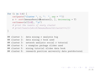
![for (i in 1:k) f
cat(paste("cluster ", i, ": ", sep = ""))
s <- sort(kmeansResult$centers[i, ], decreasing = T)
cat(names(s)[1:5], "nn")
# print the tweets of every cluster
# print(tweets[which(kmeansResult$cluster==i)])
g
## cluster 1: data mining r analysis big
## cluster 2: data mining r book used
## cluster 3: network analysis social r tutorial
## cluster 4: r examples package slides used
## cluster 5: mining tutorial slides data book
## cluster 6: research position university data postdoctoral
27 / 35](https://image.slidesharecdn.com/rdm-slides-text-mining-140915033105-phpapp01/85/Text-Mining-with-R-an-Analysis-of-Twitter-Data-28-320.jpg)
![library(fpc)
# partitioning around medoids with estimation of number of clusters
pamResult <- pamk(m3, metric="manhattan")
k <- pamResult$nc # number of clusters identified
pamResult <- pamResult$pamobject
# print cluster medoids
for (i in 1:k) f
cat("cluster", i, ": ",
colnames(pamResult$medoids)[which(pamResult$medoids[i,]==1)], "nn")
g
## cluster 1 : examples r
## cluster 2 : analysis data r
## cluster 3 : data
## cluster 4 :
## cluster 5 : r
## cluster 6 : data mining r
## cluster 7 : data mining
## cluster 8 : analysis network social
## cluster 9 : data position research
## cluster 10 : position postdoctoral university
28 / 35](https://image.slidesharecdn.com/rdm-slides-text-mining-140915033105-phpapp01/85/Text-Mining-with-R-an-Analysis-of-Twitter-Data-29-320.jpg)


![Topic Modelling
dtm <- as.DocumentTermMatrix(tdm)
library(topicmodels)
lda <- LDA(dtm, k = 8) # find 8 topics
term <- terms(lda, 4) # first 4 terms of every topic
term
## Topic 1 Topic 2 Topic 3 Topic 4
## [1,] "data" "data" "mining" "r"
## [2,] "mining" "r" "r" "lecture"
## [3,] "scientist" "mining" "tutorial" "time"
## [4,] "research" "book" "introduction" "series"
## Topic 5 Topic 6 Topic 7 Topic 8
## [1,] "position" "package" "r" "analysis"
## [2,] "research" "r" "data" "network"
## [3,] "postdoctoral" "clustering" "computing" "r"
## [4,] "university" "detection" "slides" "code"
term <- apply(term, MARGIN = 2, paste, collapse = ", ")
31 / 35](https://image.slidesharecdn.com/rdm-slides-text-mining-140915033105-phpapp01/85/Text-Mining-with-R-an-Analysis-of-Twitter-Data-32-320.jpg)
![Topic Modelling
# first topic identified for every document (tweet)
topic <- topics(lda, 1)
topics <- data.frame(date=as.IDate(tweets.df$created), topic)
qplot(date, ..count.., data=topics, geom="density",
fill=term[topic], position="stack")
0.4
0.2
0.0
2011−07 2012−01 2012−07 2013−01 2013−07
date
count
term[topic]
analysis, network, r, code
data, mining, scientist, research
data, r, mining, book
mining, r, tutorial, introduction
package, r, clustering, detection
position, research, postdoctoral, university
r, data, computing, slides
r, lecture, time, series
32 / 35](https://image.slidesharecdn.com/rdm-slides-text-mining-140915033105-phpapp01/85/Text-Mining-with-R-an-Analysis-of-Twitter-Data-33-320.jpg)


Text Mining with R -- an Analysis of Twitter Data
- 1. Text Mining with R { an Analysis of Twitter Data Yanchang Zhao http://www.RDataMining.com 30 September 2014 1 / 35
- 2. Outline Introduction Extracting Tweets Text Cleaning Frequent Words and Associations Word Cloud Clustering Topic Modelling Online Resources 2 / 35
- 3. Text Mining I unstructured text data I text categorization I text clustering I entity extraction I sentiment analysis I document summarization I . . . 3 / 35
- 4. Text mining of Twitter data with R 1 1. extract data from Twitter 2. clean extracted data and build a document-term matrix 3.
- 5. nd frequent words and associations 4. create a word cloud to visualize important words 5. text clustering 6. topic modelling 1Chapter 10: Text Mining, R and Data Mining: Examples and Case Studies. http://www.rdatamining.com/docs/RDataMining.pdf 4 / 35
- 6. Outline Introduction Extracting Tweets Text Cleaning Frequent Words and Associations Word Cloud Clustering Topic Modelling Online Resources 5 / 35
- 7. Retrieve Tweets Retrieve recent tweets by @RDataMining ## Option 1: retrieve tweets from Twitter library(twitteR) tweets <- userTimeline("RDataMining", n = 3200) ## Option 2: download @RDataMining tweets from RDataMining.com url <- "http://www.rdatamining.com/data/rdmTweets.RData" download.file(url, destfile = "./data/rdmTweets.RData") ## load tweets into R load(file = "./data/rdmTweets-201306.RData") 6 / 35
- 8. (n.tweet <- length(tweets)) ## [1] 320 tweets[1:5] ## [[1]] ## [1] "RDataMining: Examples on calling Java code from R nht... ## ## [[2]] ## [1] "RDataMining: Simulating Map-Reduce in R for Big Data A... ## ## [[3]] ## [1] "RDataMining: Job opportunity: Senior Analyst - Big Dat... ## ## [[4]] ## [1] "RDataMining: CLAVIN: an open source software package f... ## ## [[5]] ## [1] "RDataMining: An online book on Natural Language Proces... 7 / 35
- 9. Outline Introduction Extracting Tweets Text Cleaning Frequent Words and Associations Word Cloud Clustering Topic Modelling Online Resources 8 / 35
- 10. # convert tweets to a data frame # tweets.df <- do.call("rbind", lapply(tweets, as.data.frame)) tweets.df <- twListToDF(tweets) dim(tweets.df) ## [1] 320 14 library(tm) # build a corpus, and specify the source to be character vectors myCorpus <- Corpus(VectorSource(tweets.df$text)) # convert to lower case myCorpus <- tm_map(myCorpus, tolower) Package tm v0.5-10 was used in this example. With tm v0.6, content transformer" needs to be used to wrap around normal functions. # tm v0.6 myCorpus <- tm_map(myCorpus, content_transformer(tolower)) 9 / 35
- 11. # remove punctuation myCorpus <- tm_map(myCorpus, removePunctuation) # remove numbers myCorpus <- tm_map(myCorpus, removeNumbers) # remove URLs removeURL <- function(x) gsub("http[[:alnum:]]*", "", x) myCorpus <- tm_map(myCorpus, removeURL) # add two extra stop words: available and via myStopwords <- c(stopwords("english"), "available", "via") # remove r and big from stopwords myStopwords <- setdiff(myStopwords, c("r", "big")) # remove stopwords from corpus myCorpus <- tm_map(myCorpus, removeWords, myStopwords) 10 / 35
- 12. # keep a copy of corpus to use later as a dictionary for stem completion myCorpusCopy <- myCorpus # stem words myCorpus <- tm_map(myCorpus, stemDocument) # inspect the first 5 documents (tweets) inspect(myCorpus[1:5]) # The code below is used for to make text fit for paper width for (i in 1:5) f cat(paste("[[", i, "]] ", sep = "")) writeLines(myCorpus[[i]]) g ## [[1]] exampl call java code r ## ## [[2]] simul mapreduc r big data analysi use flight data ... ## [[3]] job opportun senior analyst big data wesfarm indust... ## [[4]] clavin open sourc softwar packag document geotag g... ## [[5]] onlin book natur languag process python 11 / 35
- 13. # stem completion myCorpus <- tm_map(myCorpus, stemCompletion, dictionary = myCorpusCopy) ## [[1]] examples call java code r ## [[2]] simulating mapreduce r big data analysis used flights... ## [[3]] job opportunity senior analyst big data wesfarmers in... ## [[4]] clavin open source software package document geotaggi... ## [[5]] online book natural language processing python 12 / 35
- 14. # count frequency of "mining" miningCases <- tm_map(myCorpusCopy, grep, pattern = "nn<mining") sum(unlist(miningCases)) ## [1] 82 # count frequency of "miners" minerCases <- tm_map(myCorpusCopy, grep, pattern = "nn<miners") sum(unlist(minerCases)) ## [1] 4 # replace "miners" with "mining" myCorpus <- tm_map(myCorpus, gsub, pattern = "miners", replacement = "mining") 13 / 35
- 15. tdm <- TermDocumentMatrix(myCorpus, control = list(wordLengths = c(1, Inf))) tdm ## A term-document matrix (790 terms, 320 documents) ## ## Non-/sparse entries: 2449/250351 ## Sparsity : 99% ## Maximal term length: 27 ## Weighting : term frequency (tf) 14 / 35
- 16. Outline Introduction Extracting Tweets Text Cleaning Frequent Words and Associations Word Cloud Clustering Topic Modelling Online Resources 15 / 35
- 17. idx <- which(dimnames(tdm)$Terms == "r") inspect(tdm[idx + (0:5), 101:110]) ## A term-document matrix (6 terms, 10 documents) ## ## Non-/sparse entries: 4/56 ## Sparsity : 93% ## Maximal term length: 12 ## Weighting : term frequency (tf) ## ## Docs ## Terms 101 102 103 104 105 106 107 108 109 110 ## r 0 1 1 0 0 0 0 0 1 1 ## ramachandran 0 0 0 0 0 0 0 0 0 0 ## random 0 0 0 0 0 0 0 0 0 0 ## ranked 0 0 0 0 0 0 0 0 0 0 ## rann 0 0 0 0 0 0 0 0 0 0 ## rapidminer 0 0 0 0 0 0 0 0 0 0 16 / 35
- 18. # inspect frequent words (freq.terms <- findFreqTerms(tdm, lowfreq = 15)) ## [1] "analysis" "applications" "big" "book" ## [5] "code" "computing" "data" "examples" ## [9] "group" "introduction" "mining" "network" ## [13] "package" "position" "postdoctoral" "r" ## [17] "research" "see" "slides" "social" ## [21] "tutorial" "university" "used" term.freq <- rowSums(as.matrix(tdm)) term.freq <- subset(term.freq, term.freq >= 15) df <- data.frame(term = names(term.freq), freq = term.freq) 17 / 35
- 19. library(ggplot2) ggplot(df, aes(x = term, y = freq)) + geom_bar(stat = "identity") + xlab("Terms") + ylab("Count") + coord_flip() used university tutorial social slides see research r postdoctoral position package network mining introduction group examples data computing code book big applications analysis 0 50 100 150 Count Terms 18 / 35
- 20. # which words are associated with r ? findAssocs(tdm, "r", 0.2) ## r ## examples 0.32 ## code 0.29 ## package 0.20 # which words are associated with mining ? findAssocs(tdm, "mining", 0.25) ## mining ## data 0.47 ## mahout 0.30 ## recommendation 0.30 ## sets 0.30 ## supports 0.30 ## frequent 0.26 ## itemset 0.26 19 / 35
- 21. library(graph) library(Rgraphviz) plot(tdm, term = freq.terms, corThreshold = 0.12, weighting = T) analysis research r applications big book code computing data examples group introduction mining network postdoctoral package position see slides tutorial social university used 20 / 35
- 22. Outline Introduction Extracting Tweets Text Cleaning Frequent Words and Associations Word Cloud Clustering Topic Modelling Online Resources 21 / 35
- 23. library(wordcloud) m <- as.matrix(tdm) # calculate the frequency of words and sort it by frequency word.freq <- sort(rowSums(m), decreasing = T) wordcloud(words = names(word.freq), freq = word.freq, min.freq = 3, random.order = F) language postdoctoral university social book data r project forecasting frequent applications big code tutorial job tried edited provided information research examples package mining analysis used cfp network positionslides computing see lecture introduction group analytics australia modelling scientist time association free online parallel text clustering course learn pdf rules series talk document now programming fellow statistics ausdm detection outlier google large open rdatamining techniques thanks tools users vacancy amp chapter due graphics processing notes map presentation science software starting studies visualizing business call can case center database details follower functions join kdnuggets page poll top submission spatial technology twitter analyst california card fast classification find get graph handling interactive linkedin list machine melbourne recent reference using videos web elsevier workshop wwwrdataminingcom access added canada canberra china cloud conference datasets distributed dmapps events draft experience high ibm industrial knowledge management nd performance predictive published search sentiment short snowfall southern sydney tenuretrack topic week youtube advanced also answers april area august building charts check comments containing cran create csiro dec dynamic easier engineer format guide hadoop igraph incl itemset jan labs may media microsoft mid new opportunity plot postdocresearch quick realworld san senior simple singapore state titled tj track tweets usamaf views visits watson website 22 / 35
- 24. Outline Introduction Extracting Tweets Text Cleaning Frequent Words and Associations Word Cloud Clustering Topic Modelling Online Resources 23 / 35
- 25. # remove sparse terms tdm2 <- removeSparseTerms(tdm, sparse = 0.95) m2 <- as.matrix(tdm2) # cluster terms distMatrix <- dist(scale(m2)) fit <- hclust(distMatrix, method = "ward") 24 / 35
- 26. plot(fit) rect.hclust(fit, k = 6) # cut tree into 6 clusters 10 20 30 40 50 60 research position postdoctoral university analysis network social examples package slides used computing tutorial big applications book r data mining Cluster Dendrogram Height 25 / 35
- 27. m3 <- t(m2) # transpose the matrix to cluster documents (tweets) set.seed(122) # set a fixed random seed k <- 6 # number of clusters kmeansResult <- kmeans(m3, k) round(kmeansResult$centers, digits = 3) # cluster centers ## analysis applications big book computing data examples ## 1 0.147 0.088 0.147 0.015 0.059 1.015 0.088 ## 2 0.028 0.167 0.167 0.250 0.028 1.556 0.194 ## 3 0.810 0.000 0.000 0.000 0.000 0.048 0.095 ## 4 0.080 0.036 0.007 0.058 0.087 0.000 0.181 ## 5 0.000 0.000 0.000 0.067 0.067 0.333 0.067 ## 6 0.119 0.048 0.071 0.000 0.048 0.357 0.000 ## mining network package position postdoctoral r research ## 1 0.338 0.015 0.015 0.059 0.074 0.235 0.074 ## 2 1.056 0.000 0.222 0.000 0.000 1.000 0.028 ## 3 0.048 1.000 0.095 0.143 0.095 0.286 0.048 ## 4 0.065 0.022 0.174 0.000 0.007 0.703 0.000 ## 5 1.200 0.000 0.000 0.000 0.067 0.067 0.000 ## 6 0.119 0.000 0.024 0.643 0.310 0.000 0.714 ## slides social tutorial university used ## 1 0.074 0.000 0.015 0.015 0.029 ## 2 0.056 0.000 0.000 0.000 0.250 ## 3 0.095 0.762 0.190 0.000 0.095 26 / 35
- 28. for (i in 1:k) f cat(paste("cluster ", i, ": ", sep = "")) s <- sort(kmeansResult$centers[i, ], decreasing = T) cat(names(s)[1:5], "nn") # print the tweets of every cluster # print(tweets[which(kmeansResult$cluster==i)]) g ## cluster 1: data mining r analysis big ## cluster 2: data mining r book used ## cluster 3: network analysis social r tutorial ## cluster 4: r examples package slides used ## cluster 5: mining tutorial slides data book ## cluster 6: research position university data postdoctoral 27 / 35
- 29. library(fpc) # partitioning around medoids with estimation of number of clusters pamResult <- pamk(m3, metric="manhattan") k <- pamResult$nc # number of clusters identified pamResult <- pamResult$pamobject # print cluster medoids for (i in 1:k) f cat("cluster", i, ": ", colnames(pamResult$medoids)[which(pamResult$medoids[i,]==1)], "nn") g ## cluster 1 : examples r ## cluster 2 : analysis data r ## cluster 3 : data ## cluster 4 : ## cluster 5 : r ## cluster 6 : data mining r ## cluster 7 : data mining ## cluster 8 : analysis network social ## cluster 9 : data position research ## cluster 10 : position postdoctoral university 28 / 35
- 30. # plot clustering result layout(matrix(c(1, 2), 1, 2)) # set to two graphs per page plot(pamResult, col.p = pamResult$clustering) −4 −2 0 2 4 6 −4 −2 0 2 4 clusplot(pam(x = sdata, k = k, diss = diss, metric = "manhattan")) Component 1 Component 2 These two components explain 25.23 % of the point variability. Silhouette plot of pam(x = sdata, k = k, diss = diss, metric = "manhattan") n = 320 10 clusters Cj −0.2 0.0 0.2 0.4 0.6 0.8 1.0 Silhouette width si Average silhouette width : 0.27 j : nj | aveiÎCj si 1 : 28 | 0.13 2 : 12 | 0.25 3 : 31 | 0.23 4 : 61 | 0.54 5 : 58 | 0.29 6 : 28 | 0.21 7 : 43 | 0.15 8 : 19 | 0.29 9 : 21 | 0.15 10 : 19 | 0.14 layout(matrix(1)) # change back to one graph per page 29 / 35
- 31. Outline Introduction Extracting Tweets Text Cleaning Frequent Words and Associations Word Cloud Clustering Topic Modelling Online Resources 30 / 35
- 32. Topic Modelling dtm <- as.DocumentTermMatrix(tdm) library(topicmodels) lda <- LDA(dtm, k = 8) # find 8 topics term <- terms(lda, 4) # first 4 terms of every topic term ## Topic 1 Topic 2 Topic 3 Topic 4 ## [1,] "data" "data" "mining" "r" ## [2,] "mining" "r" "r" "lecture" ## [3,] "scientist" "mining" "tutorial" "time" ## [4,] "research" "book" "introduction" "series" ## Topic 5 Topic 6 Topic 7 Topic 8 ## [1,] "position" "package" "r" "analysis" ## [2,] "research" "r" "data" "network" ## [3,] "postdoctoral" "clustering" "computing" "r" ## [4,] "university" "detection" "slides" "code" term <- apply(term, MARGIN = 2, paste, collapse = ", ") 31 / 35
- 33. Topic Modelling # first topic identified for every document (tweet) topic <- topics(lda, 1) topics <- data.frame(date=as.IDate(tweets.df$created), topic) qplot(date, ..count.., data=topics, geom="density", fill=term[topic], position="stack") 0.4 0.2 0.0 2011−07 2012−01 2012−07 2013−01 2013−07 date count term[topic] analysis, network, r, code data, mining, scientist, research data, r, mining, book mining, r, tutorial, introduction package, r, clustering, detection position, research, postdoctoral, university r, data, computing, slides r, lecture, time, series 32 / 35
- 34. Outline Introduction Extracting Tweets Text Cleaning Frequent Words and Associations Word Cloud Clustering Topic Modelling Online Resources 33 / 35
- 35. Online Resources I Chapter 10: Text Mining, in book R and Data Mining: Examples and Case Studies http://www.rdatamining.com/docs/RDataMining.pdf I R Reference Card for Data Mining http://www.rdatamining.com/docs/R-refcard-data-mining.pdf I Free online courses and documents http://www.rdatamining.com/resources/ I RDataMining Group on LinkedIn (7,000+ members) http://group.rdatamining.com I RDataMining on Twitter (1,700+ followers) @RDataMining 34 / 35
- 36. The End Thanks! Email: yanchang(at)rdatamining.com 35 / 35