The Functional Programming Triad of Map, Filter and Fold
9 likes3,653 views

This document discusses the functional programming concepts of map, filter, and fold, using examples from languages like Scheme, Clojure, Scala, Haskell, and Unison. It explores the construction of compound data structures using the pair data type, which is foundational for representing lists and hierarchical data. The text emphasizes the importance of closure property in creating complex data structures and provides insights into safe and unsafe list manipulation functions across different programming languages.


![(cons 1
(cons 2
(cons 3
(cons 4 nil))))
(1 2 3 4)
1 :: (2 :: (3 :: (4 :: Nil)))
List(1, 2, 3, 4)
cons 1
(cons 2
(cons 3
(cons 4 [])))
[1,2,3,4]
1 : (2 : (3 : (4 : [])))
[1,2,3,4]
(cons 1
(cons 2
(cons 3
(cons 4 nil))))
(1 2 3 4)](https://image.slidesharecdn.com/the-fp-triad-of-map-filter-and-fold-211101153345/85/The-Functional-Programming-Triad-of-Map-Filter-and-Fold-7-320.jpg)
![(def one-through-four `(1 2 3 4))
(first one-through-four)
1
(rest one-through-four)
(2 3 4)
(first (rest one-through-four))
2
val one_through_four = List(1, 2, 3, 4)
one_through_four.head
1
one_through_four.tail
List(2, 3, 4)
one_through_four.tail.head
2
one_through_four = [1,2,3,4]
head one_through_four
1
tail one_through_four
[2,3,4]
head (tail one_through_four)
2
(define one-through-four (list 1 2 3 4))
(car one-through-four)
1
(cdr one-through-four)
(2 3 4)
(car (cdr one-through-four))
2
What about the head and tail
functions provided by Unison?
We are not using them, because
while the Scheme, Clojure, Scala
and Haskell functions used on
the left are unsafe, the head and
tail functions provided by
Unison are safe.
For the sake of reproducing the
same behaviour as the other
functions, without getting
distracted by considerations that
are outside the scope of this
slide deck, we are just defining
our own Unison unsafe car and
cdr functions.
See the next three slides for why
the other functions are unsafe,
whereas the ones provided by
Unison are safe.
one_through_four = [1,2,3,4]
(car one_through_four)
1
(cdr one_through_four)
[2,3,4]
(car (cdr one_through_four))
2
car : [a] -> a
car xs = unsafeAt 0 xs
cdr : [a] -> [a]
cdr xs = drop 1 xs](https://image.slidesharecdn.com/the-fp-triad-of-map-filter-and-fold-211101153345/85/The-Functional-Programming-Triad-of-Map-Filter-and-Fold-8-320.jpg)
![Basic List Manipulation
The length function tells us how many elements are in a list:
ghci> :type length
length :: [a] -> Int
ghci> length []
0
ghci> length [1,2,3]
3
ghci> length "strings are lists, too"
22
If you need to determine whether a list is empty, use the null function:
ghci> :type null
null :: [a] -> Bool
ghci> null []
True
ghci> null "plugh"
False
To access the first element of a list, use the head function:
ghci> :type head
head :: [a] -> a
ghci> head [1,2,3]
1
The converse, tail, returns all but the head of a list:
ghci> :type tail
tail :: [a] -> [a]
ghci> tail "foo"
"oo”
Another function, last, returns the very last element of a list:
ghci> :type last
last :: [a] -> a
ghci> last "bar"
‘r’
The converse of last is init, which returns a list of all but the last element of its input:
ghci> :type init
init :: [a] -> [a]
ghci> init "bar"
"ba”
Several of the preceding functions behave poorly on empty lists, so be careful if
you don’t know whether or not a list is empty. What form does their misbehavior
take?
ghci> head []
*** Exception: Prelude.head: empty list
Try each of the previous functions in ghci. Which ones crash when given an empty
list?
head, tail, last and init crash.
length and null don’t.](https://image.slidesharecdn.com/the-fp-triad-of-map-filter-and-fold-211101153345/85/The-Functional-Programming-Triad-of-Map-Filter-and-Fold-9-320.jpg)

![scala> Nil.head
java.util.NoSuchElementException: head of empty list
at scala.collection.immutable.Nil$.head(List.scala:662)
... 38 elided
scala> Nil.tail
java.lang.UnsupportedOperationException: tail of empty list
at scala.collection.immutable.Nil$.tail(List.scala:664)
... 38 elided
haskell> head []
*** Exception: Prelude.head: empty list
haskell> tail []
*** Exception: Prelude.tail: empty list
clojure> (first `())
nil
clojure> (rest `())
()
scheme> (car `())
The object (), passed as the first argument to cdr, is not the correct type.
scheme> (cdr `())
The object (), passed as the first argument to cdr, is not the correct type.
def headOption: Option[A]
head :: [a] -> a
tail :: [a] -> [a]
At least Scala provides a safe
variant of the head function.
While Clojure’s first and rest functions don’t throw exceptions when invoked
on an empty sequence, they return results which, when consumed by a client,
could lead to an exception, or to some odd behaviour.
base.List.head : [a] -> Optional a
base.List.tail : [a] -> Optional [a]
Unison’s head and tail functions on the other hand, are safe in that they
return an Optional. When invoked on an empty list, rather than
throwing an exception or returning an odd result, they return None.
As we saw in the previous two slides,
Haskell’s head and tail functions throw an
exception when invoked on an empty list.](https://image.slidesharecdn.com/the-fp-triad-of-map-filter-and-fold-211101153345/85/The-Functional-Programming-Triad-of-Map-Filter-and-Fold-11-320.jpg)


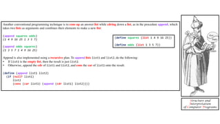
![(def squares (list 1 4 9 16 25))
(defn list-ref [items n]
(if (= n 0)
(first items)
(list-ref (rest items) (- n 1))))
val squares = List(1, 4, 9, 16, 25)
def list_ref[A](items: List[A], n: Int): A =
if n == 0
then items.head
else list_ref(items.tail, (n - 1))
squares = [1, 4, 9, 16, 25]
list_ref : [a] -> Nat -> a
list_ref items n =
if n == 0
then car items
else list_ref (cdr items) (decrement n)
squares = [1, 4, 9, 16, 25]
list_ref :: [a] -> Int -> a
list_ref items n =
if n == 0
then head items
else list_ref (tail items) (n - 1)
(define squares (list 1 4 9 16 25))
(define (list-ref items n)
(if (= n 0)
(car items)
(list-ref (cdr items) (- n 1))))](https://image.slidesharecdn.com/the-fp-triad-of-map-filter-and-fold-211101153345/85/The-Functional-Programming-Triad-of-Map-Filter-and-Fold-14-320.jpg)

![(defn length [items]
(if (empty? items)
0
(+ 1 (length (rest items)))))
def length[A](items: List[A]): Int =
if items.isEmpty
then 0
else 1 + length(items.tail)
length : [a] -> Nat
length items =
if items === empty
then 0
else 1 + (length (cdr items))
length :: [a] -> Int
length items =
if (null items)
then 0
else 1 + (length (tail items))
(define (length items)
(if (null? items)
0
(+ 1 (length (cdr items)))))](https://image.slidesharecdn.com/the-fp-triad-of-map-filter-and-fold-211101153345/85/The-Functional-Programming-Triad-of-Map-Filter-and-Fold-16-320.jpg)
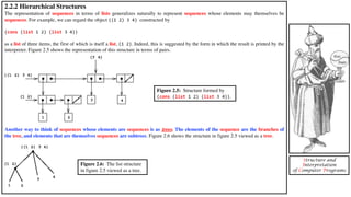
![(defn append [list1 list2]
(if (empty? list1)
list2
(cons (first list1) (append (rest list1) list2))))
def append[A](list1: List[A], list2: List[A]): List[A] =
if list1.isEmpty
then list2
else list1.head :: append(list1.tail, list2)
append : [a] -> [a] -> [a]
append list1 list2 =
if list1 === empty
then list2
else cons (car list1) (append (cdr list1) list2)
append :: [a] -> [a] -> [a]
append list1 list2 =
if (null list1)
then list2
else (head list1) : (append (tail list1) list2)
(define (append list1 list2)
(if (null? list1)
list2
(cons (car list1) (append (cdr list1) list2))))](https://image.slidesharecdn.com/the-fp-triad-of-map-filter-and-fold-211101153345/85/The-Functional-Programming-Triad-of-Map-Filter-and-Fold-18-320.jpg)

: List[B] =
if items.isEmpty
then Nil
else proc(items.head)::map(proc, items.tail)
map : (a -> b) -> [a] -> [b]
map proc items =
if items === []
then []
else cons (proc (car items))(map proc (cdr items))
map :: (a -> b) -> [a] -> [b]
map proc items =
if null items
then []
else proc (head items) : map proc (tail items)
(define (map proc items)
(if (null? items)
nil
(cons (proc (car items))
(map proc (cdr items)))))](https://image.slidesharecdn.com/the-fp-triad-of-map-filter-and-fold-211101153345/85/The-Functional-Programming-Triad-of-Map-Filter-and-Fold-20-320.jpg)

![(defn scale-list [items factor]
(map #(* % factor) items))
def scale_list(items: List[Int], factor: Int): List[Int] =
items map (_ * factor)
scale_list : [Nat] -> Nat -> [Nat]
scale_list items factor =
map (x -> x * factor) items
scale_list :: [Int] -> Int -> [Int]
scale_list items factor = map (x -> x * factor) items
(define (scale-list items factor)
(map (lambda (x) (* x factor)) items))](https://image.slidesharecdn.com/the-fp-triad-of-map-filter-and-fold-211101153345/85/The-Functional-Programming-Triad-of-Map-Filter-and-Fold-22-320.jpg)


![We have seen that in Scheme and Clojure it is straightforward to model a tree using a list: each element of the list is either a list (a
branch that is a subtree) or a value (a branch that is a leaf).
Doing so in Scala, Haskell and Unison is not so straightforward, because while Scheme and Clojure lists effortlessly support a list
element type that is either a value or a list, in order to achieve the equivalent in Scala, Haskell and Unison, some work is required.
While trees do play a role in this slide deck, it is a somewhat secondary role, so we don’t intend to translate (into our chosen
languages) all the tree-related Scheme code that we’ll be seeing.
There are however a couple of reasons why we do want to translate a small amount of tree-related code:
1) It is interesting to see how it is done
2) Later in the deck we need to be able to convert trees into lists
Consequently, we are going to introduce a simple Tree ADT (Algebraic Data Type) which is a hybrid of a tree and a list.
A tree is a list, i.e it is:
• either Null (the empty list)
• or a Leaf holding a value
• or a list of subtrees represented as a Cons (a pair) whose car is the first subtree and whose cdr is a list of the remaining subtrees.
data Tree a = Null | Leaf a | Cons (Tree a) (Tree a)
unique type Tree a = Null | Leaf a | Cons (Tree a) (Tree a)
enum Tree[+A] :
case Null
case Leaf(value: A)
case Cons(car: Tree[A], cdr: Tree[A])](https://image.slidesharecdn.com/the-fp-triad-of-map-filter-and-fold-211101153345/85/The-Functional-Programming-Triad-of-Map-Filter-and-Fold-26-320.jpg)
![count_leaves :: Tree a -> Int
count_leaves Null = 0
count_leaves (Leaf _) = 1
count_leaves (Cons car cdr) = count_leaves car +
count_leaves cdr
data Tree a = Null | Leaf a | Cons (Tree a) (Tree a)
count_leaves : Tree a -> Nat
count_leaves = cases
Null -> 0
Leaf _ -> 1
Cons car cdr -> count_leaves car +
count_leaves cdr
unique type Tree a = Null | Leaf a | Cons (Tree a) (Tree a)
(defn count-leaves [x]
(cond (not (seq? x)) 1
(empty? x) 0
:else (+ (count-leaves (first x))
(count-leaves (rest x)))))
(define (count-leaves x)
(cond ((null? x) 0)
((not (pair? x)) 1)
(else (+ (count-leaves (car x))
(count-leaves (cdr x))))))
def count_leaves[A](x: Tree[A]): Int = x match
case Null => 0
case Leaf(_) => 1
case Cons(car,cdr) => count-leaves(car) +
count-leaves(cdr)
enum Tree[+A] :
case Null
case Leaf(value: A)
case Cons(car: Tree[A], cdr: Tree[A])](https://image.slidesharecdn.com/the-fp-triad-of-map-filter-and-fold-211101153345/85/The-Functional-Programming-Triad-of-Map-Filter-and-Fold-27-320.jpg)
![x :: Tree Int
x = Cons
(Cons (Leaf 1)
(Cons (Leaf 2) Null))
(Cons (Leaf 3)
(Cons (Leaf 4) Null))
haskell> count-leaves (Cons x x)
8
x : Tree Nat
x = Cons
(Cons (Leaf 1)
(Cons (Leaf 2) Null))
(Cons (Leaf 3)
(Cons (Leaf 4) Null))
unison> count-leaves (Cons x x)
8
val x: Tree[Int] =
Cons(
Cons(Leaf(1),
Cons(Leaf(2), Null)),
Cons(Leaf(3),
Cons(Leaf(4), Null)))
scala> count-leaves( Cons(x,x) )
8
(define x
(cons
(cons 1
(cons 2 nil))
(cons 3
(cons 4 nil))))
scheme> (count-leaves (cons x x))
8
(def x
(cons
(cons 1
(cons 2 '()))
(cons 3
(cons 4 '()))))
clojure> (count-leaves (cons x x))
8](https://image.slidesharecdn.com/the-fp-triad-of-map-filter-and-fold-211101153345/85/The-Functional-Programming-Triad-of-Map-Filter-and-Fold-28-320.jpg)

![scale_tree :: Tree Int -> Int -> Tree Int
scale_tree Null factor = Null
scale_tree (Leaf a) factor = Leaf (a * factor)
scale_tree (Cons car cdr) factor = Cons (scale_tree car factor)
(scale_tree cdr factor)
scale_tree : Nat -> Tree Nat -> Tree Nat
scale_tree factor = cases
Null -> Null
(Leaf a) -> Leaf (a * factor)
(Cons car cdr) -> Cons (scale_tree factor car)
(scale_tree factor cdr)
(defn scale-tree [tree factor]
(cond (not (seq? tree)) (* tree factor)
(empty? tree) '()
:else ( (scale-tree (first tree) factor)
(scale-tree (rest tree) factor))))
(define (scale-tree tree factor)
(cond ((null? tree) nil)
((not (pair? tree)) (* tree factor))
(else (cons (scale-tree (car tree) factor)
(scale-tree (cdr tree) factor)))))
def scale_tree(tree: Tree[Int], factor: Int): Tree[Int] = tree match
case Null => Null
case Leaf(n) => Leaf(n * factor)
case Cons(car,cdr) => Cons(scale_tree(car, factor),
scale_tree(cdr, factor))](https://image.slidesharecdn.com/the-fp-triad-of-map-filter-and-fold-211101153345/85/The-Functional-Programming-Triad-of-Map-Filter-and-Fold-30-320.jpg)


: List[A] = sequence match
case Nil => Nil
case x::xs => if predicate(x)
then x::filter(predicate,xs)
else filter(predicate,xs)
filter :: (a -> Bool) -> [a] -> [a]
filter _ [] = []
filter predicate (x:xs) = if (predicate x)
then x:(filter predicate xs)
else filter predicate xs
filter : (a -> Boolean) -> [a] -> [a]
filter predicate = cases
[] -> []
x+:xs -> if (predicate x)
then x+:(filter predicate xs)
else filter predicate xs
(define (filter predicate sequence)
(cond ((null? sequence) nil)
((predicate (car sequence))
(cons (car sequence)
(filter predicate (cdr sequence))))
(else (filter predicate (cdr sequence)))))
(defn filter [predicate sequence]
(cond (empty? sequence) '()
(predicate (first sequence))
(cons (first sequence)
(filter predicate (rest sequence)))
:else (filter predicate (rest sequence))))](https://image.slidesharecdn.com/the-fp-triad-of-map-filter-and-fold-211101153345/85/The-Functional-Programming-Triad-of-Map-Filter-and-Fold-35-320.jpg)
 => B, initial: B, sequence: List[A]): B = sequence match
case Nil => initial
case x::xs => op(x,accumulate(op, initial, xs))
accumulate :: (a -> b -> b) -> b -> [a] -> b
accumulate op initial [] = initial
accumulate op initial (x:xs) = op x (accumulate op initial xs)
accumulate : (a -> b -> b) -> b -> [a] -> b
accumulate op initial = cases
[] -> initial
x+:xs -> op x (accumulate op initial xs)
(define (accumulate op initial sequence)
(if (null? sequence)
initial
(op (car sequence)
(accumulate op initial (cdr sequence)))))
(defn accumulate [op initial sequence]
(if (empty? sequence)
initial
(op (first sequence) (accumulate op initial (rest sequence)))))](https://image.slidesharecdn.com/the-fp-triad-of-map-filter-and-fold-211101153345/85/The-Functional-Programming-Triad-of-Map-Filter-and-Fold-36-320.jpg)


![∶
/
𝑥1 ∶
/
𝑥2 ∶
/
𝑥3 ∶
/
𝑥4
∶
/
𝑥1 ∶
/
𝑥2 ∶
/
𝑥3 ∶
/
𝑥4
𝑥1: (𝑥2: 𝑥3: 𝑥4: )
𝑥𝑠 = [𝑥1, 𝑥2, 𝑥3, 𝑥4] [𝑥1, 𝑥2, 𝑥3, 𝑥4]
1 : (2 : (3 : (4 : [])))
[1,2,3,4]
(cons 1
(cons 2
(cons 3
(cons 4 nil))))
(1 2 3 4)
𝑥1: (𝑥2: 𝑥3: 𝑥4: )
haskell> foldr (:) [] [1,2,3,4]
[1,2,3,4]
foldr (:) [] xs
(accumulate cons nil (list 1 2 3 4 5))
(1 2 3 4 5)
The accumulate procedure is also known as fold-right, because it combines the first
element of the sequence with the result of combining all the elements to the right.
𝑓𝑜𝑙𝑑𝑟 ∷ 𝛼 → 𝛽 → 𝛽 → 𝛽 → 𝛼 → 𝛽
𝑓𝑜𝑙𝑑𝑟 𝑓 𝑒 = 𝑒
𝑓𝑜𝑙𝑑𝑟 𝑓 𝑒 𝑥: 𝑥𝑠 = 𝑓 𝑥 𝑓𝑜𝑙𝑑𝑟 𝑓 𝑒 𝑥𝑠
Yes, accumulate cons nil, which is foldr ( : ) [ ]
in Haskell, is just the identity function on lists.
A few slides ago we saw the following
sample invocation of accumulate.
And on the previous slide we saw
that accumulate is fold-right.
𝑟𝑒𝑝𝑙𝑎𝑐𝑒:
∶ 𝑤𝑖𝑡ℎ 𝑓
𝑤𝑖𝑡ℎ 𝑒
𝑟𝑒𝑝𝑙𝑎𝑐𝑒:
∶ 𝑤𝑖𝑡ℎ ∶
𝑤𝑖𝑡ℎ](https://image.slidesharecdn.com/the-fp-triad-of-map-filter-and-fold-211101153345/85/The-Functional-Programming-Triad-of-Map-Filter-and-Fold-39-320.jpg)
![map f =
map f 𝑥 ∶ 𝑥𝑠 = 𝑓 𝑥 ∶ map 𝑓 𝑥𝑠
3ilter p =
3ilter p 𝑥 ∶ 𝑥𝑠 = 𝐢𝐟 𝑝 𝑥 𝐭𝐡𝐞𝐧 𝑥 ∶ 3ilter p 𝑥𝑠 𝐞𝐥𝐬𝐞 3ilter p 𝑥𝑠
map 𝑓 = 𝑓𝑜𝑙𝑑𝑟 𝑐𝑜𝑛𝑠 D 𝑓 𝒘𝒉𝒆𝒓𝒆 𝑐𝑜𝑛𝑠 𝑥 𝑥𝑠 = 𝑥 ∶ 𝑥𝑠 3ilter p = 𝑓𝑜𝑙𝑑𝑟 (𝜆𝑥 𝑥𝑠 → 𝐢𝐟 𝑝 𝑥 𝐭𝐡𝐞𝐧 𝑥 ∶ 𝑥𝑠 𝐞𝐥𝐬𝐞 𝑥𝑠) [ ]
map ∷ (α → 𝛽) → [α] → [𝛽] 3ilter ∷ (α → 𝐵𝑜𝑜𝑙) → [α] → [α]
By the way, it is interesting to note that map and
filter can both be defined in terms of fold-right!
So we can think of our triad’s
power as deriving entirely from
the power of folding.
fold
λ
map
λ](https://image.slidesharecdn.com/the-fp-triad-of-map-filter-and-fold-211101153345/85/The-Functional-Programming-Triad-of-Map-Filter-and-Fold-40-320.jpg)
: List[A] = tree match
case Null => Nil
case Leaf(a) => List(a)
case Cons(car,cdr) => enumerate_tree(car) ++
enumerate_tree(cdr)
enumerate_tree :: Tree a -> [a]
enumerate_tree Null = []
enumerate_tree (Leaf a) = [a]
enumerate_tree (Cons car cdr) = enumerate_tree car ++
enumerate_tree cdr
enumerate_tree : Tree a -> [a]
enumerate_tree = cases
Null -> []
Leaf a -> [a]
Cons car cdr -> enumerate_tree car ++
enumerate_tree cdr
(define (enumerate-tree tree)
(cond ((null? tree) nil)
((not (pair? tree)) (list tree))
(else (append (enumerate-tree (car tree))
(enumerate-tree (cdr tree))))))
(defn enumerate-tree [tree]
(cond (not (seq? tree)) (list tree)
(empty? tree) '()
:else (append (enumerate-tree (first tree))
(enumerate-tree (rest tree)))))
(define (enumerate-interval low high)
(if (> low high)
nil
(cons low (enumerate-interval (+ low 1) high))))
List.range(low, high+1)
[low..high]
List.range low (high+1)
(range low (inc high))](https://image.slidesharecdn.com/the-fp-triad-of-map-filter-and-fold-211101153345/85/The-Functional-Programming-Triad-of-Map-Filter-and-Fold-42-320.jpg)


![(define (sum-odd-squares tree)
(accumulate +
0
(map square
(filter odd?
(enumerate-tree tree)))))
def sum_odd_squares(tree: Tree[Int]): Int =
enumerate_tree(tree)
.filter(isOdd)
.map(square)
.foldRight(0)(_+_)
def isOdd(n: Int): Boolean = n % 2 == 1
def square(n: Int): Int = n * n
sum_odd_squares :: Tree Int -> Int
sum_odd_squares tree =
foldr (+)
0
(map square
(filter is_odd
(enumerate_tree tree)))
is_odd :: Int -> Boolean
is_odd n = (mod n 2) == 1
square :: Int -> Int
square n = n * n
sum_odd_squares : Tree Nat -> Nat
sum_odd_squares tree =
foldRight (+)
0
(map square
(filter is_odd
(enumerate_tree tree)))
is_odd : Nat -> Boolean
is_odd n = (mod n 2) == 1
square : Nat -> Nat
square n = n * n
(defn sum-odd-squares [tree]
(accumulate +
0
(map square
(filter odd? (enumerate-tree tree)))))
(defn square [n] (* n n))
(define (square n) (* n n))](https://image.slidesharecdn.com/the-fp-triad-of-map-filter-and-fold-211101153345/85/The-Functional-Programming-Triad-of-Map-Filter-and-Fold-45-320.jpg)
![(define (even-fibs n)
(accumulate cons
nil
(filter even?
(map fib
(enumerate-interval 0 n)))))
(define (fib n)
(cond ((= n 0) 0)
((= n 1) 1)
(else (+ (fib (- n 1))
(fib (- n 2))))))
(defn even-fibs [n]
(accumulate cons
'()
(filter even?
(map fib
(range 0 (inc n))))))
(defn fib [n]
(cond (= n 0) 0
(= n 1) 1
:else (+ (fib (- n 1))
(fib (- n 2)))))
def even_fibs(n: Int): List[Int] =
List.range(0,n+1)
.map(fib)
.filter(isEven)
.foldRight(List.empty[Int])(_::_)
def fib(n: Int): Int = n match def isEven(n: Int): Boolean =
case 0 => 0 n % 2 == 0
case 1 => 1
case n => fib(n-1) + fib(n-2)
even_fibs :: Int -> [Int]
even_fibs n =
foldr (:)
[]
(filter is_even
(map fib
[0..n]))
fib :: Int -> Int is_even :: Int -> Bool
fib 0 = 0 is_even n = (mod n 2) == 0
fib 1 = 1
fib n = fib (n - 1) + fib (n - 2)
even_fibs : Nat -> [Nat]
even_fibs n =
foldRight cons
[]
(filter is_even
(map fib
(range 0 (n + 1))))
fib : Nat -> Nat is_even : Nat -> Boolean
fib = cases is_even n = (mod n 2) == 0
0 -> 0
1 -> 1
n -> fib (drop n 1) + fib (drop n 2)](https://image.slidesharecdn.com/the-fp-triad-of-map-filter-and-fold-211101153345/85/The-Functional-Programming-Triad-of-Map-Filter-and-Fold-46-320.jpg)

![(define (list-fib-squares n)
(accumulate cons
nil
(map square
(map fib
(enumerate-interval 0 n)))))
(defn list-fib-squares [n]
(accumulate cons
'()
(map square
(map fib
(range 0 (inc n))))))
def list_fib_squares(n: Int): List[Int] =
List.range(0,n+1)
.map(fib)
.map(square)
.foldRight(List.empty[Int])(_::_)
list_fib_squares :: Int -> [Int]
list_fib_squares n =
foldr (:)
[]
(map square
(map fib
[0..n]))
list_fib_squares : Nat -> [Nat]
list_fib_squares n =
foldRight cons
[]
(map square
(map fib
(range 0 (n + 1))))
(define (fib n) (define (square n) (* n n))
(cond ((= n 0) 0)
((= n 1) 1)
(else (+ (fib (- n 1))
(fib (- n 2))))))
(defn fib [n] (defn square [n] (* n n))
(cond (= n 0) 0
(= n 1) 1
:else (+ (fib (- n 1))
(fib (- n 2)))))
def fib(n: Int): Int = n match def square(n: Int): Int =
case 0 => 0 n * n
case 1 => 1
case n => fib(n-1) + fib(n-2)
fib :: Int -> Int square :: Int -> Int
fib 0 = 0 square n = n * n
fib 1 = 1
fib n = fib (n - 1) + fib (n - 2)
fib : Nat -> Nat square : Nat -> Nat
fib = cases square n = n * n
0 -> 0
1 -> 1
n -> fib (drop n 1) + fib (drop n 2)](https://image.slidesharecdn.com/the-fp-triad-of-map-filter-and-fold-211101153345/85/The-Functional-Programming-Triad-of-Map-Filter-and-Fold-48-320.jpg)
![(define (product-of-squares-of-odd-elements sequence)
(accumulate *
1
(map square
(filter odd? sequence))))
(defn product-of-squares-of-odd-elements [sequence]
(accumulate *
1
(map square
(filter odd? sequence))))
def product_of_squares_of_odd_elements(sequence: List[Int]): Int =
sequence.filter(isOdd)
.map(square)
.foldRight(1)(_*_)
product_of_squares_of_odd_elements :: [Int] -> Int
product_of_squares_of_odd_elements sequence =
foldr (*)
1
(map square
(filter is_odd
sequence))
product_of_squares_of_odd_elements : [Nat] -> Nat
product_of_squares_of_odd_elements sequence =
foldRight (*)
1
(map square
(filter is_odd
sequence))
(define (square n) (* n n))
(defn square [n] (* n n))
def isOdd(n: Int): Boolean = n % 2 == 1
def square(n: Int): Int = n * n
is_odd :: Int -> Boolean
is_odd n = (mod n 2) == 1
square :: Int -> Int
square n = n * n
is_odd : Nat -> Boolean
is_odd n = (mod n 2) == 1
square : Nat -> Nat
square n = n * n](https://image.slidesharecdn.com/the-fp-triad-of-map-filter-and-fold-211101153345/85/The-Functional-Programming-Triad-of-Map-Filter-and-Fold-49-320.jpg)


The Functional Programming Triad of Map, Filter and Fold
- 1. Unison map λ Clojure Haskell Scala Scheme Structure and Interpretation of Computer Programs @philip_schwarz slides by https://www.slideshare.net/pjschwarz The Functional Programming Triad of map, filter and fold Polyglot FP for Fun and Profit – Scheme, Clojure, Scala, Haskell, Unison closely based on the book Structure and Interpretation of Computer Programs SICP
- 2. This slide deck is my homage to SICP, the book which first introduced me to the Functional Programming triad of map, filter and fold. It was during my Computer Science degree that a fellow student gave me a copy of the first edition, not long after the book came out. I have not yet come across a better introduction to these three functions. The upcoming slides are closely based on the second edition of the book, a free online copy of which can be found here: https://mitpress.mit.edu/sites/default/files/sicp/full-text/book/book.html. @philip_schwarz
- 3. Pairs To enable us to implement the concrete level of our data abstraction, our language provides a compound structure called a pair, which can be constructed with the primitive procedure cons. This procedure takes two arguments and returns a compound data object that contains the two arguments as parts. Given a pair, we can extract the parts using the primitive procedures car and cdr. Thus, we can use cons, car, and cdr as follows: (define x (cons 1 2)) (car x) 1 (cdr x) 2 Notice that a pair is a data object that can be given a name and manipulated, just like a primitive data object. Moreover, cons can be used to form pairs whose elements are pairs, and so on: (define x (cons 1 2)) (define y (cons 3 4)) (define z (cons x y)) (car (car z)) 1 (car (cdr z)) 3 In section 2.2 we will see how this ability to combine pairs means that pairs can be used as general-purpose building blocks to create all sorts of complex data structures. The single compound-data primitive pair, implemented by the procedures cons, car, and cdr, is the only glue we need. Data objects constructed from pairs are called list-structured data. Structure and Interpretation of Computer Programs The name cons stands for construct. The names car and cdr derive from the original implementation of Lisp on the IBM 704. That machine had an addressing scheme that allowed one to reference the address and decrement parts of a memory location. car stands for Contents of Address part of Register and cdr (pronounced could-er) stands for Contents of Decrement part of Register.
- 4. 2.2 Hierarchical Data and the Closure Property As we have seen, pairs provide a primitive glue that we can use to construct compound data objects. Figure 2.2 shows a standard way to visualize a pair -- in this case, the pair formed by (cons 1 2). In this representation, which is called box-and-pointer notation, each object is shown as a pointer to a box. The box for a primitive object contains a representation of the object. For example, the box for a number contains a numeral. The box for a pair is actually a double box, the left part containing (a pointer to) the car of the pair and the right part containing the cdr. We have already seen that cons can be used to combine not only numbers but pairs as well. … As a consequence, pairs provide a universal building block from which we can construct all sorts of data structures. Figure 2.3 shows two ways to use pairs to combine the numbers 1, 2, 3, and 4. Structure and Interpretation of Computer Programs
- 5. The ability to create pairs whose elements are pairs is the essence of list structure's importance as a representational tool. We refer to this ability as the closure property of cons. In general, an operation for combining data objects satisfies the closure property if the results of combining things with that operation can themselves be combined filter using the same operation. Closure is the key to power in any means of combination because it permits us to create hierarchical structures -- structures made up of parts, which themselves are made up of parts, and so on. From the outset of chapter 1, we've made essential use of closure in dealing with procedures, because all but the very simplest programs rely on the fact that the elements of a combination can themselves be combinations. In this section, we take up the consequences of closure for compound data. We describe some conventional techniques for using pairs to represent sequences and trees, and we exhibit a graphics language that illustrates closure in a vivid way. 2.2.1 Representing Sequences Figure 2.4: The sequence 1,2,3,4 represented as a chain of pairs. One of the useful structures we can build with pairs is a sequence -- an ordered collection of data objects. There are, of course, many ways to represent sequences in terms of pairs. One particularly straightforward representation is illustrated in figure 2.4, where the sequence 1, 2, 3, 4 is represented as a chain of pairs. The car of each pair is the corresponding item in the chain, and the cdr of the pair is the next pair in the chain. The cdr of the final pair signals the end of the sequence by pointing to a distinguished value that is not a pair, represented in box-and-pointer diagrams as a diagonal line and in programs as the value of the variable nil. The entire sequence is constructed by nested cons operations: (cons 1 (cons 2 (cons 3 (cons 4 nil)))) Structure and Interpretation of Computer Programs
- 6. Such a sequence of pairs, formed by nested conses, is called a list, and Scheme provides a primitive called list to help in constructing lists. The above sequence could be produced by (list 1 2 3 4). In general, (list <a1> <a2> ... <an>) is equivalent to (cons <a1> (cons <a2> (cons ... (cons <an> nil) ...))) Lisp systems conventionally print lists by printing the sequence of elements, enclosed in parentheses. Thus, the data object in figure 2.4 is printed as (1 2 3 4): (define one-through-four (list 1 2 3 4)) one-through-four (1 2 3 4) Be careful not to confuse the expression (list 1 2 3 4) with the list (1 2 3 4), which is the result obtained when the expression is evaluated. Attempting to evaluate the expression (1 2 3 4) will signal an error when the interpreter tries to apply the procedure 1 to arguments 2, 3, and 4. We can think of car as selecting the first item in the list, and of cdr as selecting the sublist consisting of all but the first item. Nested applications of car and cdr can be used to extract the second, third, and subsequent items in the list. The constructor cons makes a list like the original one, but with an additional item at the beginning. (car one-through-four) 1 (cdr one-through-four) (2 3 4) Structure and Interpretation of Computer Programs Figure 2.4: The sequence 1,2,3,4 represented as a chain of pairs.
- 7. (cons 1 (cons 2 (cons 3 (cons 4 nil)))) (1 2 3 4) 1 :: (2 :: (3 :: (4 :: Nil))) List(1, 2, 3, 4) cons 1 (cons 2 (cons 3 (cons 4 []))) [1,2,3,4] 1 : (2 : (3 : (4 : []))) [1,2,3,4] (cons 1 (cons 2 (cons 3 (cons 4 nil)))) (1 2 3 4)
- 8. (def one-through-four `(1 2 3 4)) (first one-through-four) 1 (rest one-through-four) (2 3 4) (first (rest one-through-four)) 2 val one_through_four = List(1, 2, 3, 4) one_through_four.head 1 one_through_four.tail List(2, 3, 4) one_through_four.tail.head 2 one_through_four = [1,2,3,4] head one_through_four 1 tail one_through_four [2,3,4] head (tail one_through_four) 2 (define one-through-four (list 1 2 3 4)) (car one-through-four) 1 (cdr one-through-four) (2 3 4) (car (cdr one-through-four)) 2 What about the head and tail functions provided by Unison? We are not using them, because while the Scheme, Clojure, Scala and Haskell functions used on the left are unsafe, the head and tail functions provided by Unison are safe. For the sake of reproducing the same behaviour as the other functions, without getting distracted by considerations that are outside the scope of this slide deck, we are just defining our own Unison unsafe car and cdr functions. See the next three slides for why the other functions are unsafe, whereas the ones provided by Unison are safe. one_through_four = [1,2,3,4] (car one_through_four) 1 (cdr one_through_four) [2,3,4] (car (cdr one_through_four)) 2 car : [a] -> a car xs = unsafeAt 0 xs cdr : [a] -> [a] cdr xs = drop 1 xs
- 9. Basic List Manipulation The length function tells us how many elements are in a list: ghci> :type length length :: [a] -> Int ghci> length [] 0 ghci> length [1,2,3] 3 ghci> length "strings are lists, too" 22 If you need to determine whether a list is empty, use the null function: ghci> :type null null :: [a] -> Bool ghci> null [] True ghci> null "plugh" False To access the first element of a list, use the head function: ghci> :type head head :: [a] -> a ghci> head [1,2,3] 1 The converse, tail, returns all but the head of a list: ghci> :type tail tail :: [a] -> [a] ghci> tail "foo" "oo” Another function, last, returns the very last element of a list: ghci> :type last last :: [a] -> a ghci> last "bar" ‘r’ The converse of last is init, which returns a list of all but the last element of its input: ghci> :type init init :: [a] -> [a] ghci> init "bar" "ba” Several of the preceding functions behave poorly on empty lists, so be careful if you don’t know whether or not a list is empty. What form does their misbehavior take? ghci> head [] *** Exception: Prelude.head: empty list Try each of the previous functions in ghci. Which ones crash when given an empty list? head, tail, last and init crash. length and null don’t.
- 10. Partial and Total Functions Functions that have only return values defined for a subset of valid inputs are called partial functions (calling error doesn’t qualify as returning a value!). We call functions that return valid results over their entire input domains total functions. It’s always a good idea to know whether a function you’re using is partial or total. Calling a partial function with an input that it can’t handle is probably the single biggest source of straightforward, avoidable bugs in Haskell programs. Some Haskell programmers go so far as to give partial functions names that begin with a prefix such as unsafe so that they can’t shoot themselves in the foot accidentally. It’s arguably a deficiency of the standard Prelude that it defines quite a few “unsafe” partial functions, such as head, without also providing “safe” total equivalents.
- 11. scala> Nil.head java.util.NoSuchElementException: head of empty list at scala.collection.immutable.Nil$.head(List.scala:662) ... 38 elided scala> Nil.tail java.lang.UnsupportedOperationException: tail of empty list at scala.collection.immutable.Nil$.tail(List.scala:664) ... 38 elided haskell> head [] *** Exception: Prelude.head: empty list haskell> tail [] *** Exception: Prelude.tail: empty list clojure> (first `()) nil clojure> (rest `()) () scheme> (car `()) The object (), passed as the first argument to cdr, is not the correct type. scheme> (cdr `()) The object (), passed as the first argument to cdr, is not the correct type. def headOption: Option[A] head :: [a] -> a tail :: [a] -> [a] At least Scala provides a safe variant of the head function. While Clojure’s first and rest functions don’t throw exceptions when invoked on an empty sequence, they return results which, when consumed by a client, could lead to an exception, or to some odd behaviour. base.List.head : [a] -> Optional a base.List.tail : [a] -> Optional [a] Unison’s head and tail functions on the other hand, are safe in that they return an Optional. When invoked on an empty list, rather than throwing an exception or returning an odd result, they return None. As we saw in the previous two slides, Haskell’s head and tail functions throw an exception when invoked on an empty list.
- 12. (car (cdr one-through-four)) 2 (cons 10 one-through-four) (10 1 2 3 4) (cons 5 one-through-four) (5 1 2 3 4) The value of nil, used to terminate the chain of pairs, can be thought of as a sequence of no elements, the empty list. The word nil is a contraction of the Latin word nihil, which means nothing. Structure and Interpretation of Computer Programs It's remarkable how much energy in the standardization of Lisp dialects has been dissipated in arguments that are literally over nothing: Should nil be an ordinary name? Should the value of nil be a symbol? Should it be a list? Should it be a pair? In Scheme, nil is an ordinary name, which we use in this section as a variable whose value is the end-of-list marker (just as true is an ordinary variable that has a true value). Other dialects of Lisp, including Common Lisp, treat nil as a special symbol. The authors of this book, who have endured too many language standardization brawls, would like to avoid the entire issue. Once we have introduced quotation in section 2.3, we will denote the empty list as '() and dispense with the variable nil entirely.
- 13. List Operations The use of pairs to represent sequences of elements as lists is accompanied by conventional programming techniques for manipulating lists by successively cdring down' the lists. For example, the procedure list-ref takes as arguments a list and a number n and returns the nth item of the list. It is customary to number the elements of the list beginning with 0. The method for computing list-ref is the following: • For n = 0, list-ref should return the car of the list. • Otherwise, list-ref should return the (n - 1)st item of the cdr of the list. (define (list-ref items n) (if (= n 0) (car items) (list-ref (cdr items) (- n 1)))) (define squares (list 1 4 9 16 25)) (list-ref squares 3) 16 Structure and Interpretation of Computer Programs
- 14. (def squares (list 1 4 9 16 25)) (defn list-ref [items n] (if (= n 0) (first items) (list-ref (rest items) (- n 1)))) val squares = List(1, 4, 9, 16, 25) def list_ref[A](items: List[A], n: Int): A = if n == 0 then items.head else list_ref(items.tail, (n - 1)) squares = [1, 4, 9, 16, 25] list_ref : [a] -> Nat -> a list_ref items n = if n == 0 then car items else list_ref (cdr items) (decrement n) squares = [1, 4, 9, 16, 25] list_ref :: [a] -> Int -> a list_ref items n = if n == 0 then head items else list_ref (tail items) (n - 1) (define squares (list 1 4 9 16 25)) (define (list-ref items n) (if (= n 0) (car items) (list-ref (cdr items) (- n 1))))
- 15. Often we cdr down the whole list. To aid in this, Scheme includes a primitive predicate null?, which tests whether its argument is the empty list. The procedure length, which returns the number of items in a list, illustrates this typical pattern of use: (define (length items) (if (null? items) 0 (+ 1 (length (cdr items))))) (define odds (list 1 3 5 7)) (length odds) 4 The length procedure implements a simple recursive plan. The reduction step is: • The length of any list is 1 plus the length of the cdr of the list. This is applied successively until we reach the base case: • The length of the empty list is 0. We could also compute length in an iterative style: (define (length items) (define (length-iter a count) (if (null? a) count (length-iter (cdr a) (+ 1 count)))) (length-iter items 0)) Structure and Interpretation of Computer Programs
- 16. (defn length [items] (if (empty? items) 0 (+ 1 (length (rest items))))) def length[A](items: List[A]): Int = if items.isEmpty then 0 else 1 + length(items.tail) length : [a] -> Nat length items = if items === empty then 0 else 1 + (length (cdr items)) length :: [a] -> Int length items = if (null items) then 0 else 1 + (length (tail items)) (define (length items) (if (null? items) 0 (+ 1 (length (cdr items)))))
- 17. Another conventional programming technique is to cons up an answer list while cdring down a list, as in the procedure append, which takes two lists as arguments and combines their elements to make a new list: (append squares odds) (1 4 9 16 25 1 3 5 7) (append odds squares) (1 3 5 7 1 4 9 16 25) Append is also implemented using a recursive plan. To append lists list1 and list2, do the following: • If list1 is the empty list, then the result is just list2. • Otherwise, append the cdr of list1 and list2, and cons the car of list1 onto the result: (define (append list1 list2) (if (null? list1) list2 (cons (car list1) (append (cdr list1) list2)))) Structure and Interpretation of Computer Programs (define squares (list 1 4 9 16 25)) (define odds (list 1 3 5 7))
- 18. (defn append [list1 list2] (if (empty? list1) list2 (cons (first list1) (append (rest list1) list2)))) def append[A](list1: List[A], list2: List[A]): List[A] = if list1.isEmpty then list2 else list1.head :: append(list1.tail, list2) append : [a] -> [a] -> [a] append list1 list2 = if list1 === empty then list2 else cons (car list1) (append (cdr list1) list2) append :: [a] -> [a] -> [a] append list1 list2 = if (null list1) then list2 else (head list1) : (append (tail list1) list2) (define (append list1 list2) (if (null? list1) list2 (cons (car list1) (append (cdr list1) list2))))
- 19. Mapping Over Lists One extremely useful operation is to apply some transformation to each element in a list and generate the list of results. For instance, the following procedure scales each number in a list by a given factor: (define (scale-list items factor) (if (null? items) nil (cons (* (car items) factor) (scale-list (cdr items) factor)))) (scale-list (list 1 2 3 4 5) 10) (10 20 30 40 50) We can abstract this general idea and capture it as a common pattern expressed as a higher-order procedure, just as in section 1.3. The higher-order procedure here is called map. Map takes as arguments a procedure of one argument and a list, and returns a list of the results produced by applying the procedure to each element in the list: (define (map proc items) (if (null? items) nil (cons (proc (car items)) (map proc (cdr items))))) (map abs (list -10 2.5 -11.6 17)) (10 2.5 11.6 17) (map (lambda (x) (* x x)) (list 1 2 3 4)) (1 4 9 16) Structure and Interpretation of Computer Programs
- 20. (define (map proc items) (if (null? items) '() (cons (proc (car items))(map proc(cdr items))))) def map[A,B](proc: A => B, items: List[A]): List[B] = if items.isEmpty then Nil else proc(items.head)::map(proc, items.tail) map : (a -> b) -> [a] -> [b] map proc items = if items === [] then [] else cons (proc (car items))(map proc (cdr items)) map :: (a -> b) -> [a] -> [b] map proc items = if null items then [] else proc (head items) : map proc (tail items) (define (map proc items) (if (null? items) nil (cons (proc (car items)) (map proc (cdr items)))))
- 21. Now we can give a new definition of scale-list in terms of map: (define (scale-list items factor) (map (lambda (x) (* x factor)) items)) Map is an important construct, not only because it captures a common pattern, but because it establishes a higher level of abstraction in dealing with lists. In the original definition of scale-list, the recursive structure of the program draws attention to the element-by-element processing of the list. Defining scale-list in terms of map suppresses that level of detail and emphasizes that scaling transforms a list of elements to a list of results. The difference between the two definitions is not that the computer is performing a different process (it isn't) but that we think about the process differently. In effect, map helps establish an abstraction barrier that isolates the implementation of procedures that transform lists from the details of how the elements of the list are extracted and combined. Like the barriers shown in figure 2.1, this abstraction gives us the flexibility to change the low-level details of how sequences are implemented, while preserving the conceptual framework of operations that transform sequences to sequences. Section 2.2.3 expands on this use of sequences as a framework for organizing programs. Structure and Interpretation of Computer Programs (define (scale-list items factor) (if (null? items) nil (cons (* (car items) factor) (scale-list (cdr items) factor))))
- 22. (defn scale-list [items factor] (map #(* % factor) items)) def scale_list(items: List[Int], factor: Int): List[Int] = items map (_ * factor) scale_list : [Nat] -> Nat -> [Nat] scale_list items factor = map (x -> x * factor) items scale_list :: [Int] -> Int -> [Int] scale_list items factor = map (x -> x * factor) items (define (scale-list items factor) (map (lambda (x) (* x factor)) items))
- 23. map λ map is the first function in the functional programming triad that we are covering in this slide deck. @philip_schwarz
- 24. 2.2.2 Hierarchical Structures The representation of sequences in terms of lists generalizes naturally to represent sequences whose elements may themselves be sequences. For example, we can regard the object ((1 2) 3 4) constructed by (cons (list 1 2) (list 3 4)) as a list of three items, the first of which is itself a list, (1 2). Indeed, this is suggested by the form in which the result is printed by the interpreter. Figure 2.5 shows the representation of this structure in terms of pairs. Another way to think of sequences whose elements are sequences is as trees. The elements of the sequence are the branches of the tree, and elements that are themselves sequences are subtrees. Figure 2.6 shows the structure in figure 2.5 viewed as a tree. Structure and Interpretation of Computer Programs Figure 2.5: Structure formed by (cons (list 1 2) (list 3 4)). Figure 2.6: The list structure in figure 2.5 viewed as a tree.
- 25. Recursion is a natural tool for dealing with tree structures, since we can often reduce operations on trees to operations on their branches, which reduce in turn to operations on the branches of the branches, and so on, until we reach the leaves of the tree. As an example, compare the length procedure of section 2.2.1 with the count-leaves procedure, which returns the total number of leaves of a tree: (define x (cons (list 1 2) (list 3 4))) (length x) 3 (count-leaves x) 4 (list x x) (((1 2) 3 4) ((1 2) 3 4)) (length (list x x)) 2 (count-leaves (list x x)) 8 But in the reduction step, where we strip off the car of the list, we must take into account that the car may itself be a tree whose leaves we need to count. Thus, the appropriate reduction step is • count-leaves of a tree x is count-leaves of the car of x plus count-leaves of the cdr of x. Finally, by taking cars we reach actual leaves, so we need another base case: • count-leaves of a leaf is 1. To aid in writing recursive procedures on trees, Scheme provides the primitive predicate pair?, which tests whether its argument is a pair. Here is the complete procedure: (define (count-leaves x) (cond ((null? x) 0) ((not (pair? x)) 1) (else (+ (count-leaves (car x)) (count-leaves (cdr x)))))) Structure and Interpretation of Computer Programs (define (length items) (if (null? items) 0 (+ 1 (length (cdr items))))) To implement count-leaves, recall the recursive plan for computing length: • Length of a list x is 1 plus length of the cdr of x. • Length of the empty list is 0. count-leaves is similar. The value for the empty list is the same: • count-leaves of the empty list is 0.
- 26. We have seen that in Scheme and Clojure it is straightforward to model a tree using a list: each element of the list is either a list (a branch that is a subtree) or a value (a branch that is a leaf). Doing so in Scala, Haskell and Unison is not so straightforward, because while Scheme and Clojure lists effortlessly support a list element type that is either a value or a list, in order to achieve the equivalent in Scala, Haskell and Unison, some work is required. While trees do play a role in this slide deck, it is a somewhat secondary role, so we don’t intend to translate (into our chosen languages) all the tree-related Scheme code that we’ll be seeing. There are however a couple of reasons why we do want to translate a small amount of tree-related code: 1) It is interesting to see how it is done 2) Later in the deck we need to be able to convert trees into lists Consequently, we are going to introduce a simple Tree ADT (Algebraic Data Type) which is a hybrid of a tree and a list. A tree is a list, i.e it is: • either Null (the empty list) • or a Leaf holding a value • or a list of subtrees represented as a Cons (a pair) whose car is the first subtree and whose cdr is a list of the remaining subtrees. data Tree a = Null | Leaf a | Cons (Tree a) (Tree a) unique type Tree a = Null | Leaf a | Cons (Tree a) (Tree a) enum Tree[+A] : case Null case Leaf(value: A) case Cons(car: Tree[A], cdr: Tree[A])
- 27. count_leaves :: Tree a -> Int count_leaves Null = 0 count_leaves (Leaf _) = 1 count_leaves (Cons car cdr) = count_leaves car + count_leaves cdr data Tree a = Null | Leaf a | Cons (Tree a) (Tree a) count_leaves : Tree a -> Nat count_leaves = cases Null -> 0 Leaf _ -> 1 Cons car cdr -> count_leaves car + count_leaves cdr unique type Tree a = Null | Leaf a | Cons (Tree a) (Tree a) (defn count-leaves [x] (cond (not (seq? x)) 1 (empty? x) 0 :else (+ (count-leaves (first x)) (count-leaves (rest x))))) (define (count-leaves x) (cond ((null? x) 0) ((not (pair? x)) 1) (else (+ (count-leaves (car x)) (count-leaves (cdr x)))))) def count_leaves[A](x: Tree[A]): Int = x match case Null => 0 case Leaf(_) => 1 case Cons(car,cdr) => count-leaves(car) + count-leaves(cdr) enum Tree[+A] : case Null case Leaf(value: A) case Cons(car: Tree[A], cdr: Tree[A])
- 28. x :: Tree Int x = Cons (Cons (Leaf 1) (Cons (Leaf 2) Null)) (Cons (Leaf 3) (Cons (Leaf 4) Null)) haskell> count-leaves (Cons x x) 8 x : Tree Nat x = Cons (Cons (Leaf 1) (Cons (Leaf 2) Null)) (Cons (Leaf 3) (Cons (Leaf 4) Null)) unison> count-leaves (Cons x x) 8 val x: Tree[Int] = Cons( Cons(Leaf(1), Cons(Leaf(2), Null)), Cons(Leaf(3), Cons(Leaf(4), Null))) scala> count-leaves( Cons(x,x) ) 8 (define x (cons (cons 1 (cons 2 nil)) (cons 3 (cons 4 nil)))) scheme> (count-leaves (cons x x)) 8 (def x (cons (cons 1 (cons 2 '())) (cons 3 (cons 4 '())))) clojure> (count-leaves (cons x x)) 8
- 29. Mapping over trees Just as map is a powerful abstraction for dealing with sequences, map together with recursion is a powerful abstraction for dealing with trees. For instance, the scale-tree procedure, analogous to scale-list of section 2.2.1, takes as arguments a numeric factor and a tree whose leaves are numbers. It returns a tree of the same shape, where each number is multiplied by the factor. The recursive plan for scale-tree is similar to the one for count-leaves: (define (scale-tree tree factor) (cond ((null? tree) nil) ((not (pair? tree)) (* tree factor)) (else (cons (scale-tree (car tree) factor) (scale-tree (cdr tree) factor))))) (scale-tree (list 1 (list 2 (list 3 4) 5) (list 6 7)) 10) (10 (20 (30 40) 50) (60 70)) Another way to implement scale-tree is to regard the tree as a sequence of sub-trees and use map. We map over the sequence, scaling each sub-tree in turn, and return the list of results. In the base case, where the tree is a leaf, we simply multiply by the factor: (define (scale-tree tree factor) (map (lambda (sub-tree) (if (pair? sub-tree) (scale-tree sub-tree factor) (* sub-tree factor))) tree)) Many tree operations can be implemented by similar combinations of sequence operations and recursion. Structure and Interpretation of Computer Programs (define (count-leaves x) (cond ((null? x) 0) ((not (pair? x)) 1) (else (+ (count-leaves (car x)) (count-leaves (cdr x)))))) (define (scale-list items factor) (if (null? items) nil (cons (* (car items) factor) (scale-list (cdr items) factor)))) Note that while representing trees using our Tree ADT means that we are able to translate the above scale-tree function into our chosen languages (see next slide), the same is not true of the scale-tree function on the left, because map takes as a parameter not a Tree ADT but a list.
- 30. scale_tree :: Tree Int -> Int -> Tree Int scale_tree Null factor = Null scale_tree (Leaf a) factor = Leaf (a * factor) scale_tree (Cons car cdr) factor = Cons (scale_tree car factor) (scale_tree cdr factor) scale_tree : Nat -> Tree Nat -> Tree Nat scale_tree factor = cases Null -> Null (Leaf a) -> Leaf (a * factor) (Cons car cdr) -> Cons (scale_tree factor car) (scale_tree factor cdr) (defn scale-tree [tree factor] (cond (not (seq? tree)) (* tree factor) (empty? tree) '() :else ( (scale-tree (first tree) factor) (scale-tree (rest tree) factor)))) (define (scale-tree tree factor) (cond ((null? tree) nil) ((not (pair? tree)) (* tree factor)) (else (cons (scale-tree (car tree) factor) (scale-tree (cdr tree) factor))))) def scale_tree(tree: Tree[Int], factor: Int): Tree[Int] = tree match case Null => Null case Leaf(n) => Leaf(n * factor) case Cons(car,cdr) => Cons(scale_tree(car, factor), scale_tree(cdr, factor))
- 31. 2.2.3 Sequences as Conventional Interfaces In working with compound data, we've stressed how data abstraction permits us to design programs without becoming enmeshed in the details of data representations, and how abstraction preserves for us the flexibility to experiment with alternative representations. In this section, we introduce another powerful design principle for working with data structures -- the use of conventional interfaces. In section 1.3 we saw how program abstractions, implemented as higher-order procedures, can capture common patterns in programs that deal with numerical data. Our ability to formulate analogous operations for working with compound data depends crucially on the style in which we manipulate our data structures. Consider, for example, the following procedure, analogous to the count-leaves procedure of section 2.2.2, which takes a tree as argument and computes the sum of the squares of the leaves that are odd: (define (sum-odd-squares tree) (cond ((null? tree) 0) ((not (pair? tree)) (if (odd? tree) (square tree) 0)) (else (+ (sum-odd-squares (car tree)) (sum-odd-squares (cdr tree)))))) On the surface, this procedure is very different from the following one, which constructs a list of all the even Fibonacci numbers Fib(k), where k is less than or equal to a given integer n : (define (even-fibs n) (define (next k) (if (> k n) nil (let ((f (fib k))) (if (even? f) (cons f (next (+ k 1))) (next (+ k 1)))))) (next 0)) Structure and Interpretation of Computer Programs (define (count-leaves x) (cond ((null? x) 0) ((not (pair? x)) 1) (else (+ (count-leaves (car x)) (count-leaves (cdr x))))))
- 32. Despite the fact that these two procedures are structurally very different, a more abstract description of the two computations reveals a great deal of similarity. The first program • enumerates the leaves of a tree; • filters them, selecting the odd ones; • squares each of the selected ones; and • accumulates the results using +, starting with 0. The second program • enumerates the integers from 0 to n; • computes the Fibonacci number for each integer; • filters them, selecting the even ones; and • accumulates the results using cons, starting with the empty list. A signal-processing engineer would find it natural to conceptualize these processes in terms of signals flowing through a cascade of stages, each of which implements part of the program plan, as shown in figure 2.7. In sum-odd-squares, we begin with an enumerator, which generates a signal consisting of the leaves of a given tree. This signal is passed through a filter, which eliminates all but the odd elements. The resulting signal is in turn passed through a map, which is a transducer that applies the square procedure to each element. The output of the map is then fed to an accumulator, which combines the elements using +, starting from an initial 0. The plan for even-fibs is analogous. Structure and Interpretation of Computer Programs (define (sum-odd-squares tree) (cond ((null? tree) 0) ((not (pair? tree)) (if (odd? tree) (square tree) 0)) (else (+ (sum-odd-squares (car tree)) (sum-odd-squares (cdr tree)))))) (define (even-fibs n) (define (next k) (if (> k n) nil (let ((f (fib k))) (if (even? f) (cons f (next (+ k 1))) (next (+ k 1)))))) (next 0)) enumerate: tree leaves filter: odd? map: square accumulate: +, 0 enumerate: integers map: fib filter: even? accumulate: cons, () Figure 2.7: The signal-flow plans for the procedures sum- odd-squares (top) and even-fibs (bottom) reveal the commonality between the two programs.
- 33. Structure and Interpretation of Computer Programs Unfortunately, the two procedure definitions above fail to exhibit this signal-flow structure. For instance, if we examine the sum-odd-squares procedure, we find that the enumeration is implemented partly by the null? and pair? tests and partly by the tree-recursive structure of the procedure. (define (sum-odd-squares tree) (cond ((null? tree) 0) ((not (pair? tree)) (if (odd? tree) (square tree) 0)) (else (+ (sum-odd-squares (car tree)) (sum-odd-squares (cdr tree)))))) Similarly, the accumulation is found partly in the tests and partly in the addition used in the recursion. In general, there are no distinct parts of either procedure that correspond to the elements in the signal-flow description. Our two procedures decompose the computations in a different way, spreading the enumeration over the program and mingling it with the map, the filter, and the accumulation. If we could organize our programs to make the signal-flow structure manifest in the procedures we write, this would increase the conceptual clarity of the resulting code. enumerate: tree leaves filter: odd? map: square accumulate: +, 0
- 34. Sequence Operations The key to organizing programs so as to more clearly reflect the signal-flow structure is to concentrate on the signals that flow from one stage in the process to the next. If we represent these signals as lists, then we can use list operations to implement the processing at each of the stages. For instance, we can implement the mapping stages of the signal-flow diagrams using the map procedure from section 2.2.1: (map square (list 1 2 3 4 5)) (1 4 9 16 25) filtering a sequence to select only those elements that satisfy a given predicate is accomplished by (define (filter predicate sequence) (cond ((null? sequence) nil) ((predicate (car sequence)) (cons (car sequence) (filter predicate (cdr sequence)))) (else (filter predicate (cdr sequence))))) For example, (filter odd? (list 1 2 3 4 5)) (1 3 5) accumulations can be implemented by (define (accumulate op initial sequence) (if (null? sequence) initial (op (car sequence) (accumulate op initial (cdr sequence))))) Structure and Interpretation of Computer Programs (accumulate * 1 (list 1 2 3 4 5)) 120 (accumulate cons nil (list 1 2 3 4 5)) (1 2 3 4 5) (accumulate + 0 (list 1 2 3 4 5)) 15
- 35. def filter[A](predicate: A => Boolean, sequence: List[A]): List[A] = sequence match case Nil => Nil case x::xs => if predicate(x) then x::filter(predicate,xs) else filter(predicate,xs) filter :: (a -> Bool) -> [a] -> [a] filter _ [] = [] filter predicate (x:xs) = if (predicate x) then x:(filter predicate xs) else filter predicate xs filter : (a -> Boolean) -> [a] -> [a] filter predicate = cases [] -> [] x+:xs -> if (predicate x) then x+:(filter predicate xs) else filter predicate xs (define (filter predicate sequence) (cond ((null? sequence) nil) ((predicate (car sequence)) (cons (car sequence) (filter predicate (cdr sequence)))) (else (filter predicate (cdr sequence))))) (defn filter [predicate sequence] (cond (empty? sequence) '() (predicate (first sequence)) (cons (first sequence) (filter predicate (rest sequence))) :else (filter predicate (rest sequence))))
- 36. def accumulate[A,B](op: (A,B) => B, initial: B, sequence: List[A]): B = sequence match case Nil => initial case x::xs => op(x,accumulate(op, initial, xs)) accumulate :: (a -> b -> b) -> b -> [a] -> b accumulate op initial [] = initial accumulate op initial (x:xs) = op x (accumulate op initial xs) accumulate : (a -> b -> b) -> b -> [a] -> b accumulate op initial = cases [] -> initial x+:xs -> op x (accumulate op initial xs) (define (accumulate op initial sequence) (if (null? sequence) initial (op (car sequence) (accumulate op initial (cdr sequence))))) (defn accumulate [op initial sequence] (if (empty? sequence) initial (op (first sequence) (accumulate op initial (rest sequence)))))
- 37. filter and fold are the other two functions in our FP triad. map λ The accumulate procedure is also known as fold-right, because it combines the first element of the sequence with the result of combining all the elements to the right. There is also a fold-left, which is similar to fold-right, except that it combines elements working in the opposite direction: (define (fold-left op initial sequence) (define (iter result rest) (if (null? rest) result (iter (op result (car rest)) (cdr rest)))) (iter initial sequence)) Structure and Interpretation of Computer Programs
- 38. If you want to know more about left and right folds then see below for a whole series of slide decks dedicated to folding. @philip_schwarz
- 39. ∶ / 𝑥1 ∶ / 𝑥2 ∶ / 𝑥3 ∶ / 𝑥4 ∶ / 𝑥1 ∶ / 𝑥2 ∶ / 𝑥3 ∶ / 𝑥4 𝑥1: (𝑥2: 𝑥3: 𝑥4: ) 𝑥𝑠 = [𝑥1, 𝑥2, 𝑥3, 𝑥4] [𝑥1, 𝑥2, 𝑥3, 𝑥4] 1 : (2 : (3 : (4 : []))) [1,2,3,4] (cons 1 (cons 2 (cons 3 (cons 4 nil)))) (1 2 3 4) 𝑥1: (𝑥2: 𝑥3: 𝑥4: ) haskell> foldr (:) [] [1,2,3,4] [1,2,3,4] foldr (:) [] xs (accumulate cons nil (list 1 2 3 4 5)) (1 2 3 4 5) The accumulate procedure is also known as fold-right, because it combines the first element of the sequence with the result of combining all the elements to the right. 𝑓𝑜𝑙𝑑𝑟 ∷ 𝛼 → 𝛽 → 𝛽 → 𝛽 → 𝛼 → 𝛽 𝑓𝑜𝑙𝑑𝑟 𝑓 𝑒 = 𝑒 𝑓𝑜𝑙𝑑𝑟 𝑓 𝑒 𝑥: 𝑥𝑠 = 𝑓 𝑥 𝑓𝑜𝑙𝑑𝑟 𝑓 𝑒 𝑥𝑠 Yes, accumulate cons nil, which is foldr ( : ) [ ] in Haskell, is just the identity function on lists. A few slides ago we saw the following sample invocation of accumulate. And on the previous slide we saw that accumulate is fold-right. 𝑟𝑒𝑝𝑙𝑎𝑐𝑒: ∶ 𝑤𝑖𝑡ℎ 𝑓 𝑤𝑖𝑡ℎ 𝑒 𝑟𝑒𝑝𝑙𝑎𝑐𝑒: ∶ 𝑤𝑖𝑡ℎ ∶ 𝑤𝑖𝑡ℎ
- 40. map f = map f 𝑥 ∶ 𝑥𝑠 = 𝑓 𝑥 ∶ map 𝑓 𝑥𝑠 3ilter p = 3ilter p 𝑥 ∶ 𝑥𝑠 = 𝐢𝐟 𝑝 𝑥 𝐭𝐡𝐞𝐧 𝑥 ∶ 3ilter p 𝑥𝑠 𝐞𝐥𝐬𝐞 3ilter p 𝑥𝑠 map 𝑓 = 𝑓𝑜𝑙𝑑𝑟 𝑐𝑜𝑛𝑠 D 𝑓 𝒘𝒉𝒆𝒓𝒆 𝑐𝑜𝑛𝑠 𝑥 𝑥𝑠 = 𝑥 ∶ 𝑥𝑠 3ilter p = 𝑓𝑜𝑙𝑑𝑟 (𝜆𝑥 𝑥𝑠 → 𝐢𝐟 𝑝 𝑥 𝐭𝐡𝐞𝐧 𝑥 ∶ 𝑥𝑠 𝐞𝐥𝐬𝐞 𝑥𝑠) [ ] map ∷ (α → 𝛽) → [α] → [𝛽] 3ilter ∷ (α → 𝐵𝑜𝑜𝑙) → [α] → [α] By the way, it is interesting to note that map and filter can both be defined in terms of fold-right! So we can think of our triad’s power as deriving entirely from the power of folding. fold λ map λ
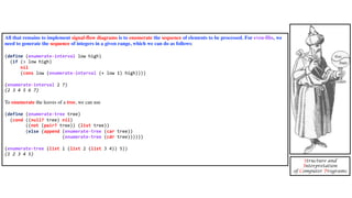
- 41. All that remains to implement signal-flow diagrams is to enumerate the sequence of elements to be processed. For even-fibs, we need to generate the sequence of integers in a given range, which we can do as follows: (define (enumerate-interval low high) (if (> low high) nil (cons low (enumerate-interval (+ low 1) high)))) (enumerate-interval 2 7) (2 3 4 5 6 7) To enumerate the leaves of a tree, we can use (define (enumerate-tree tree) (cond ((null? tree) nil) ((not (pair? tree)) (list tree)) (else (append (enumerate-tree (car tree)) (enumerate-tree (cdr tree)))))) (enumerate-tree (list 1 (list 2 (list 3 4)) 5)) (1 2 3 4 5) Structure and Interpretation of Computer Programs
- 42. def enumerate_tree[A](tree: Tree[A]): List[A] = tree match case Null => Nil case Leaf(a) => List(a) case Cons(car,cdr) => enumerate_tree(car) ++ enumerate_tree(cdr) enumerate_tree :: Tree a -> [a] enumerate_tree Null = [] enumerate_tree (Leaf a) = [a] enumerate_tree (Cons car cdr) = enumerate_tree car ++ enumerate_tree cdr enumerate_tree : Tree a -> [a] enumerate_tree = cases Null -> [] Leaf a -> [a] Cons car cdr -> enumerate_tree car ++ enumerate_tree cdr (define (enumerate-tree tree) (cond ((null? tree) nil) ((not (pair? tree)) (list tree)) (else (append (enumerate-tree (car tree)) (enumerate-tree (cdr tree)))))) (defn enumerate-tree [tree] (cond (not (seq? tree)) (list tree) (empty? tree) '() :else (append (enumerate-tree (first tree)) (enumerate-tree (rest tree))))) (define (enumerate-interval low high) (if (> low high) nil (cons low (enumerate-interval (+ low 1) high)))) List.range(low, high+1) [low..high] List.range low (high+1) (range low (inc high))
- 43. Now we can reformulate sum-odd-squares and even-fibs as in the signal-flow diagrams. For sum-odd-squares, we enumerate the sequence of leaves of the tree, filter this to keep only the odd numbers in the sequence, square each element, and sum the results: (define (sum-odd-squares tree) (accumulate + 0 (map square (filter odd? (enumerate-tree tree))))) For even-fibs, we enumerate the integers from 0 to n, generate the Fibonacci number for each of these integers, filter the resulting sequence to keep only the even elements, and accumulate the results into a list: (define (even-fibs n) (accumulate cons nil (filter even? (map fib (enumerate-interval 0 n))))) The value of expressing programs as sequence operations is that this helps us make program designs that are modular, that is, designs that are constructed by combining relatively independent pieces. We can encourage modular design by providing a library of standard components together with a conventional interface for connecting the components in flexible ways. Structure and Interpretation of Computer Programs enumerate: tree leaves filter: odd? map: square accumulate: +, 0 (define (sum-odd-squares tree) (cond ((null? tree) 0) ((not (pair? tree)) (if (odd? tree) (square tree) 0)) (else (+ (sum-odd-squares (car tree)) (sum-odd-squares (cdr tree)))))) enumerate: integers map: fib filter: even? accumulate: cons, () (define (even-fibs n) (define (next k) (if (> k n) nil (let ((f (fib k))) (if (even? f) (cons f (next (+ k 1))) (next (+ k 1)))))) (next 0))
- 44. list op signal = list enumerate: tree leaves filter: odd? map: square accumulate: +, 0 list op list op enumerate: integers map: fib filter: even? accumulate: cons, () (define (sum-odd-squares tree) (accumulate + 0 (map square (filter odd? (enumerate-tree tree))))) (define (even-fibs n) (accumulate cons nil (filter even? (map fib (enumerate-interval 0 n))))) At first sight the two programs don’t appear to have much in common, but if we refactor them, modularising them according to the signal flow structure of the computation that they perform, then we do see the commonality between the programs. The new modularisation also increases the conceptual clarity of the programs. (define (sum-odd-squares tree) (cond ((null? tree) 0) ((not (pair? tree)) (if (odd? tree) (square tree) 0)) (else (+ (sum-odd-squares (car tree)) (sum-odd-squares (cdr tree)))))) (define (even-fibs n) (define (next k) (if (> k n) nil (let ((f (fib k))) (if (even? f) (cons f (next (+ k 1))) (next (+ k 1)))))) (next 0)) The refactored programs perform signal processing: • each program is a cascade of signal processing stages • signals are represented as lists • signals flow from one stage of the process to the next • list operations represent the processing at each stage map λ
- 45. (define (sum-odd-squares tree) (accumulate + 0 (map square (filter odd? (enumerate-tree tree))))) def sum_odd_squares(tree: Tree[Int]): Int = enumerate_tree(tree) .filter(isOdd) .map(square) .foldRight(0)(_+_) def isOdd(n: Int): Boolean = n % 2 == 1 def square(n: Int): Int = n * n sum_odd_squares :: Tree Int -> Int sum_odd_squares tree = foldr (+) 0 (map square (filter is_odd (enumerate_tree tree))) is_odd :: Int -> Boolean is_odd n = (mod n 2) == 1 square :: Int -> Int square n = n * n sum_odd_squares : Tree Nat -> Nat sum_odd_squares tree = foldRight (+) 0 (map square (filter is_odd (enumerate_tree tree))) is_odd : Nat -> Boolean is_odd n = (mod n 2) == 1 square : Nat -> Nat square n = n * n (defn sum-odd-squares [tree] (accumulate + 0 (map square (filter odd? (enumerate-tree tree))))) (defn square [n] (* n n)) (define (square n) (* n n))
- 46. (define (even-fibs n) (accumulate cons nil (filter even? (map fib (enumerate-interval 0 n))))) (define (fib n) (cond ((= n 0) 0) ((= n 1) 1) (else (+ (fib (- n 1)) (fib (- n 2)))))) (defn even-fibs [n] (accumulate cons '() (filter even? (map fib (range 0 (inc n)))))) (defn fib [n] (cond (= n 0) 0 (= n 1) 1 :else (+ (fib (- n 1)) (fib (- n 2))))) def even_fibs(n: Int): List[Int] = List.range(0,n+1) .map(fib) .filter(isEven) .foldRight(List.empty[Int])(_::_) def fib(n: Int): Int = n match def isEven(n: Int): Boolean = case 0 => 0 n % 2 == 0 case 1 => 1 case n => fib(n-1) + fib(n-2) even_fibs :: Int -> [Int] even_fibs n = foldr (:) [] (filter is_even (map fib [0..n])) fib :: Int -> Int is_even :: Int -> Bool fib 0 = 0 is_even n = (mod n 2) == 0 fib 1 = 1 fib n = fib (n - 1) + fib (n - 2) even_fibs : Nat -> [Nat] even_fibs n = foldRight cons [] (filter is_even (map fib (range 0 (n + 1)))) fib : Nat -> Nat is_even : Nat -> Boolean fib = cases is_even n = (mod n 2) == 0 0 -> 0 1 -> 1 n -> fib (drop n 1) + fib (drop n 2)
- 47. Modular construction is a powerful strategy for controlling complexity in engineering design. In real signal-processing applications, for example, designers regularly build systems by cascading elements selected from standardized families of filters and transducers. Similarly, sequence operations provide a library of standard program elements that we can mix and match. For instance, we can reuse pieces from the sum-odd-squares and even-fibs procedures in a program that constructs a list of the squares of the first n + 1 Fibonacci numbers: (define (list-fib-squares n) (accumulate cons nil (map square (map fib (enumerate-interval 0 n))))) (list-fib-squares 10) (0 1 1 4 9 25 64 169 441 1156 3025) We can rearrange the pieces and use them in computing the product of the odd integers in a sequence: (define (product-of-squares-of-odd-elements sequence) (accumulate * 1 (map square (filter odd? sequence)))) (product-of-squares-of-odd-elements (list 1 2 3 4 5)) 225 Structure and Interpretation of Computer Programs enumerate: integers map: fib map: square accumulate: cons, () enumerate: sequence filter: odd? map: square accumulate: *, 1 (define (even-fibs n) (accumulate cons nil (filter even? (map fib (enumerate-interval 0 n))))) (define (sum-odd-squares tree) (accumulate + 0 (map square (filter odd? (enumerate-tree tree)))))
- 48. (define (list-fib-squares n) (accumulate cons nil (map square (map fib (enumerate-interval 0 n))))) (defn list-fib-squares [n] (accumulate cons '() (map square (map fib (range 0 (inc n)))))) def list_fib_squares(n: Int): List[Int] = List.range(0,n+1) .map(fib) .map(square) .foldRight(List.empty[Int])(_::_) list_fib_squares :: Int -> [Int] list_fib_squares n = foldr (:) [] (map square (map fib [0..n])) list_fib_squares : Nat -> [Nat] list_fib_squares n = foldRight cons [] (map square (map fib (range 0 (n + 1)))) (define (fib n) (define (square n) (* n n)) (cond ((= n 0) 0) ((= n 1) 1) (else (+ (fib (- n 1)) (fib (- n 2)))))) (defn fib [n] (defn square [n] (* n n)) (cond (= n 0) 0 (= n 1) 1 :else (+ (fib (- n 1)) (fib (- n 2))))) def fib(n: Int): Int = n match def square(n: Int): Int = case 0 => 0 n * n case 1 => 1 case n => fib(n-1) + fib(n-2) fib :: Int -> Int square :: Int -> Int fib 0 = 0 square n = n * n fib 1 = 1 fib n = fib (n - 1) + fib (n - 2) fib : Nat -> Nat square : Nat -> Nat fib = cases square n = n * n 0 -> 0 1 -> 1 n -> fib (drop n 1) + fib (drop n 2)
- 49. (define (product-of-squares-of-odd-elements sequence) (accumulate * 1 (map square (filter odd? sequence)))) (defn product-of-squares-of-odd-elements [sequence] (accumulate * 1 (map square (filter odd? sequence)))) def product_of_squares_of_odd_elements(sequence: List[Int]): Int = sequence.filter(isOdd) .map(square) .foldRight(1)(_*_) product_of_squares_of_odd_elements :: [Int] -> Int product_of_squares_of_odd_elements sequence = foldr (*) 1 (map square (filter is_odd sequence)) product_of_squares_of_odd_elements : [Nat] -> Nat product_of_squares_of_odd_elements sequence = foldRight (*) 1 (map square (filter is_odd sequence)) (define (square n) (* n n)) (defn square [n] (* n n)) def isOdd(n: Int): Boolean = n % 2 == 1 def square(n: Int): Int = n * n is_odd :: Int -> Boolean is_odd n = (mod n 2) == 1 square :: Int -> Int square n = n * n is_odd : Nat -> Boolean is_odd n = (mod n 2) == 1 square : Nat -> Nat square n = n * n
- 50. Structure and Interpretation of Computer Programs We can also formulate conventional data-processing applications in terms of sequence operations. Suppose we have a sequence of personnel records and we want to find the salary of the highest-paid programmer. Assume that we have a selector salary that returns the salary of a record, and a predicate programmer? that tests if a record is for a programmer. Then we can write (define (salary-of-highest-paid-programmer records) (accumulate max 0 (map salary (filter programmer? records)))) These examples give just a hint of the vast range of operations that can be expressed as sequence operations. Sequences, implemented here as lists, serve as a conventional interface that permits us to combine processing modules. Additionally, when we uniformly represent structures as sequences, we have localized the data-structure dependencies in our programs to a small number of sequence operations. By changing these, we can experiment with alternative representations of sequences, while leaving the overall design of our programs intact. enumerate: records filter: programmer? map: salary accumulate: max, 0
- 51. To be continued in Part 2 map λ @philip_schwarz