SlideShare a Scribd company logo
Time and Space Complexity
Dr. Ashutosh Satapathy
Assistant Professor, Department of CSE
VR Siddhartha Engineering College
Kanuru, Vijayawada
September 25, 2022
Dr. Ashutosh Satapathy Time and Space Complexity September 25, 2022 1 / 50
Outline
1 Algorithm Analysis
Time and Space Complexity
Time Complexity
Space Complexity
2 Asymptotic Notation
Basics
Asymptote
Big-Oh notation
Big Omega notation
Little-Oh notation
Little-Omega notation
Theta notation
Limit Definition
3 Complexity Analysis
Growth of Functions
Types of Time Complexities
Time Complexity Analysis
Space Complexity Analysis
Dr. Ashutosh Satapathy Time and Space Complexity September 25, 2022 2 / 50
Outline
1 Algorithm Analysis
Time and Space Complexity
Time Complexity
Space Complexity
2 Asymptotic Notation
Basics
Asymptote
Big-Oh notation
Big Omega notation
Little-Oh notation
Little-Omega notation
Theta notation
Limit Definition
3 Complexity Analysis
Growth of Functions
Types of Time Complexities
Time Complexity Analysis
Space Complexity Analysis
Dr. Ashutosh Satapathy Time and Space Complexity September 25, 2022 3 / 50
Time and Space Complexity
Designing an efficient algorithm for a program plays a crucial role in a
large scale computer system.
Time complexity and space complexity are the two most important
considerations for deciding the efficiency of an algorithm.
The time complexity of an algorithm is the number of instructions
that it needs to run to completion.
The space complexity of an algorithm is the amount of memory that
it needs to run to completion.
The analysis of running time generally has received more attention
than memory because any program that uses huge amounts of
memory automatically requires a lot of time.
Dr. Ashutosh Satapathy Time and Space Complexity September 25, 2022 4 / 50
Outline
1 Algorithm Analysis
Time and Space Complexity
Time Complexity
Space Complexity
2 Asymptotic Notation
Basics
Asymptote
Big-Oh notation
Big Omega notation
Little-Oh notation
Little-Omega notation
Theta notation
Limit Definition
3 Complexity Analysis
Growth of Functions
Types of Time Complexities
Time Complexity Analysis
Space Complexity Analysis
Dr. Ashutosh Satapathy Time and Space Complexity September 25, 2022 5 / 50
Time Complexity
In analyzing algorithm we will not consider the following information
although they are very important.
1 The machine we are executing on.
2 The machine language instruction set.
3 The time required by each machine instruction
4 The translation, a compiler will make from the source to the machine
language.
The exact time we determine would no apply to many machines.
There would be the problem of the compiler which could vary from
machine to machine.
It is often difficult to get reliable timing figures because of clock
limitations and a multi-programming or time sharing environment.
We will concentrate on developing only the frequency count for all
statements.
Dr. Ashutosh Satapathy Time and Space Complexity September 25, 2022 6 / 50
Time Complexity
1: x ← x + 1 ▷ Frequency count is 1
1: for I ← 1 to n do ▷ Frequency count is n+1
2: x ← x + 1; ▷ Frequency count is n
3: end for
1: for I ← 1 to n do ▷ Frequency count is n+1
2: for J ← 1 to n do ▷ Frequency count is n(n+1)
3: x ← x + 1; ▷ Frequency count is n2
4: end for
5: end for
Dr. Ashutosh Satapathy Time and Space Complexity September 25, 2022 7 / 50
Time Complexity
Algorithm 1 Fibonacci sequence
1: procedure Fibonacci(n)
2: if (n < 0) then
3: write (”error”)
4: return
5: end if
6: if (n = 0) then
7: write 0
8: return
9: end if
10: if (n = 1) then
11: write 1
12: return
13: end if
14: fnm2 ← 0
15: fnm1 ← 1
16: for I ← 2 to n do
17: fn ← fnm1 + fnm2
18: fnm2 ← fnm1
19: fnm2 ← fn
20: end for
21: write fn
22: end procedure
Dr. Ashutosh Satapathy Time and Space Complexity September 25, 2022 8 / 50
Time Complexity
Table 1.1: Frequency count for computing Fn in Fibonacci series
Step n <0 n = 0 n = 1 n Step n <0 n = 0 n = 1 n
1 1 1 1 1 12 0 0 1 0
2 1 1 1 1 13 0 0 0 0
3 1 0 0 0 14 0 0 0 1
4 1 0 0 0 15 0 0 0 1
5 0 0 0 0 16 0 0 0 n
6 0 1 1 1 17 0 0 0 n-1
7 0 1 0 0 18 0 0 0 n-1
8 0 1 0 0 19 0 0 0 n-1
9 0 0 0 0 20 0 0 0 n-1
10 0 0 1 1 21 0 0 0 1
11 0 0 1 0 22 0 0 0 1
Frequency Count 4 5 6 5n+4
Dr. Ashutosh Satapathy Time and Space Complexity September 25, 2022 9 / 50
Outline
1 Algorithm Analysis
Time and Space Complexity
Time Complexity
Space Complexity
2 Asymptotic Notation
Basics
Asymptote
Big-Oh notation
Big Omega notation
Little-Oh notation
Little-Omega notation
Theta notation
Limit Definition
3 Complexity Analysis
Growth of Functions
Types of Time Complexities
Time Complexity Analysis
Space Complexity Analysis
Dr. Ashutosh Satapathy Time and Space Complexity September 25, 2022 10 / 50
Space Complexity
The space needed by a program is the sum of the following components.
Fixed space requirement: The component refers to space
requirement that do not depend on the number and size of the
program’s inputs and outputs. The fixed requirements include the
instruction space (space needed to store the code), space for simple
variables, fixed size structured variable and constants.
Variable space requirement: This component consists of the space
needed by structured variables whose size depends on the particular
instance i, of the problem being solved. It also includes the
additional space required when a function uses recursion.
The space requirement S(P) of an algorithm P may therefore be written
as S(P) = c + SP, where c and SP are the constant and instance
characteristics, respectively. First, we need to determine which instance
characteristics to use for a give problem to reduce the space requirements.
Dr. Ashutosh Satapathy Time and Space Complexity September 25, 2022 11 / 50
Space Complexity
Algorithm 2 Square of the given Number
1: procedure getsquare(n)
2: return n*n
3: end procedure
We can solve the problem without consuming any extra space, hence the
space complexity is constant.
Dr. Ashutosh Satapathy Time and Space Complexity September 25, 2022 12 / 50
Space Complexity
Algorithm 3 Sum of array elements
1: procedure calculate sum(A, n)
2: sum ← 0
3: for i ← 0 to n − 1 do
4: sum ← sum + A[i]
5: end for
6: end procedure
n, sum and i take constant sum of 3 units, but the variable A is an array,
it’s space consumption increases with the increase of input size n.
Dr. Ashutosh Satapathy Time and Space Complexity September 25, 2022 13 / 50
Outline
1 Algorithm Analysis
Time and Space Complexity
Time Complexity
Space Complexity
2 Asymptotic Notation
Basics
Asymptote
Big-Oh notation
Big Omega notation
Little-Oh notation
Little-Omega notation
Theta notation
Limit Definition
3 Complexity Analysis
Growth of Functions
Types of Time Complexities
Time Complexity Analysis
Space Complexity Analysis
Dr. Ashutosh Satapathy Time and Space Complexity September 25, 2022 14 / 50
Basics
The main idea of asymptotic analysis is to have a measure of
efficiency of algorithms that doesn’t depend on machine specific
constants.
Asymptotic analysis of an algorithm refers to defining the
mathematical boundation/framing of its run-time performance.
It doesn’t require algorithms to be implemented and time taken by
programs to be compared.
Asymptotic notations are mathematical tools to represent time
complexity of algorithms for asymptotic analysis.
Dr. Ashutosh Satapathy Time and Space Complexity September 25, 2022 15 / 50
Outline
1 Algorithm Analysis
Time and Space Complexity
Time Complexity
Space Complexity
2 Asymptotic Notation
Basics
Asymptote
Big-Oh notation
Big Omega notation
Little-Oh notation
Little-Omega notation
Theta notation
Limit Definition
3 Complexity Analysis
Growth of Functions
Types of Time Complexities
Time Complexity Analysis
Space Complexity Analysis
Dr. Ashutosh Satapathy Time and Space Complexity September 25, 2022 16 / 50
Asymptote
A ’Line’ that continually approaches a given curve but does not meet
it at any finite distance.
The term asymptotic means approaching a value or curve arbitrarily
closely (i.e., as some sort of limit is taken).
A line or a curve A that is asymptotic to given curve C is called the
asymptote of C.
Figure 2.1: Asymptote of curve f(x)
Dr. Ashutosh Satapathy Time and Space Complexity September 25, 2022 17 / 50
Outline
1 Algorithm Analysis
Time and Space Complexity
Time Complexity
Space Complexity
2 Asymptotic Notation
Basics
Asymptote
Big-Oh notation
Big Omega notation
Little-Oh notation
Little-Omega notation
Theta notation
Limit Definition
3 Complexity Analysis
Growth of Functions
Types of Time Complexities
Time Complexity Analysis
Space Complexity Analysis
Dr. Ashutosh Satapathy Time and Space Complexity September 25, 2022 18 / 50
O (Big-Oh) notation
Big-Oh is used as a tight upper-bound on the growth of an
algorithm’s effort (this effort is described by the function f(n)).
Let f(n) and g(n) be functions that map positive integers to positive
real numbers. We say that f(n) is O(g(n)) or f(n) ∈ O(g(n)), if
there exists a real constant c > 0 and there exists an integer constant
n0 ≥ 1 such that f(n) ≤ cg(n) for every integer n ≥ n0.
In other words O(g(n)) = {f(n): there exist positive constants c and
n0 such that 0 ≤ f(n) ≤ cg(n) for all n ≥ n0}
Figure 2.2: f(n) ∈ O(g(n))
Dr. Ashutosh Satapathy Time and Space Complexity September 25, 2022 19 / 50
O (Big-Oh) notation
Question 1: Consider the function f(n) = 6n+ 135. Clearly. f(n) is
non-negative for all integers n ≥ 0. We wish to show that f(n)=O(n2).
According to the Big-oh definition, in order to show this we need to find
an integer n0, and a constant c > 0 such that for all integers, n ≥ n0, f(n)
= c(n2)
Answer: Suppose we choose c = 1, and f(n) = cn2.
⇒ 6n+135 = cn2 = n2 [Since c = 1] n2-6n-135 = 0
⇒ (n-15)(n+9) = 0
Since (n+9) > 0 for all values n ≥ 0, we conclude that (n-15) = 0
⇒ n0 = 15 for c = 1
For c = 2, n0 = (6 +
√
1116)/4 ≈ 9.9
For c = 4, n0 = (6 +
√
2196)/8 ≈ 6.7
Dr. Ashutosh Satapathy Time and Space Complexity September 25, 2022 20 / 50
Outline
1 Algorithm Analysis
Time and Space Complexity
Time Complexity
Space Complexity
2 Asymptotic Notation
Basics
Asymptote
Big-Oh notation
Big Omega notation
Little-Oh notation
Little-Omega notation
Theta notation
Limit Definition
3 Complexity Analysis
Growth of Functions
Types of Time Complexities
Time Complexity Analysis
Space Complexity Analysis
Dr. Ashutosh Satapathy Time and Space Complexity September 25, 2022 21 / 50
Ω (Big-Omega) notation
Big-Omega (Ω) is the tight lower bound notation.
Let f(n) and g(n) be functions that map positive integers to positive
real numbers. We say that f(n) is Ω(g(n)) or f(n) ∈ Ω(g(n)) if
there exists a real constant c > 0 and there exists an integer constant
n0 ≥ 1 such that f(n) ≥ cg(n) for every integer n ≥ n0.
In other words Ω(g(n)) = {f(n): there exist positive constants c and
n0 such that 0 ≤ cg(n) ≤ f(n) for all n ≥ n0}.
Figure 2.3: f(n) ∈ Ω(g(n))
Dr. Ashutosh Satapathy Time and Space Complexity September 25, 2022 22 / 50
Ω (Big-Omega) notation
Question 2: Consider the function f(n)= 3n2-24n+72. Clearly f(n) is
non-negative for all integers n ≥ 0. We wish to show that f(n) = Ω(n2).
According to the big-omega definition, in order to show this we need to
find an integer n0,and a constant c > 0 such that for all integers n = n0,
f(n) = cn2.
Answer: Suppose we choosc c = 1, Then f(n) = cn2
⇒ 3n2-24n+72 = n2
⇒ 2n2-24n+72 = 0
⇒ 2(n-6)2 = 0
Since (n-6)2 = 0, we conclude that n0 = 6.
So we have that for c = 1 and n ≥ 6, f(n) = cn2. Hence f(n) = Ω(n2).
Dr. Ashutosh Satapathy Time and Space Complexity September 25, 2022 23 / 50
Outline
1 Algorithm Analysis
Time and Space Complexity
Time Complexity
Space Complexity
2 Asymptotic Notation
Basics
Asymptote
Big-Oh notation
Big Omega notation
Little-Oh notation
Little-Omega notation
Theta notation
Limit Definition
3 Complexity Analysis
Growth of Functions
Types of Time Complexities
Time Complexity Analysis
Space Complexity Analysis
Dr. Ashutosh Satapathy Time and Space Complexity September 25, 2022 24 / 50
o (Little-Oh) notation
Little-oh (o) is used as a loose upper-bound on the growth of an
algorithm’s effort (this effort is described by the function f(n)).
Let f(n) and g(n) be functions that map positive integers to positive
real numbers. We say that f(n) is o(g(n)) or f(n) ∈ o(g(n)) if for
any real constant c > 0, there exists an integer constant n0 ≥ 1 such
that f(n) < cg(n) for every integer n ≥ n0.
In other words o(g(n)) = {f(n): there exist positive constants c and
n0 such that 0 ≤ f(n) < cg(n) for all n ≥ n0}.
Figure 2.4: f(n) ∈ o(g(n))
Dr. Ashutosh Satapathy Time and Space Complexity September 25, 2022 25 / 50
Outline
1 Algorithm Analysis
Time and Space Complexity
Time Complexity
Space Complexity
2 Asymptotic Notation
Basics
Asymptote
Big-Oh notation
Big Omega notation
Little-Oh notation
Little-Omega notation
Theta notation
Limit Definition
3 Complexity Analysis
Growth of Functions
Types of Time Complexities
Time Complexity Analysis
Space Complexity Analysis
Dr. Ashutosh Satapathy Time and Space Complexity September 25, 2022 26 / 50
ω (Little-Omega) notation
Little Omega (ω) is used as a loose lower-bound on the growth of
an algorithm’s effort (this effort is described by the function f(n)).
Let f(n) and g(n) be functions that map positive integers to positive
real numbers. We say that f(n) is ω(g(n)) or f(n) ∈ ω(g(n)) if for
any real constant c > 0, there exists an integer constant n0 ≥ 1 such
that f(n) > cg(n) for every integer n ≥ n0.
In other words ω(g(n)) = {f(n): there exist positive constants c and
n0 such that 0 ≤ cg(n) < f(n) for all n ≥ n0}.
Figure 2.5: f(n) ∈ ω(g(n))
Dr. Ashutosh Satapathy Time and Space Complexity September 25, 2022 27 / 50
Outline
1 Algorithm Analysis
Time and Space Complexity
Time Complexity
Space Complexity
2 Asymptotic Notation
Basics
Asymptote
Big-Oh notation
Big Omega notation
Little-Oh notation
Little-Omega notation
Theta notation
Limit Definition
3 Complexity Analysis
Growth of Functions
Types of Time Complexities
Time Complexity Analysis
Space Complexity Analysis
Dr. Ashutosh Satapathy Time and Space Complexity September 25, 2022 28 / 50
θ (Theta) notation
Let f(n) and g(n) be functions that map positive integers to positive
real numbers. We say that f(n) is θ(g(n)) or f(n) ∈ θ(g(n)) if and
only if f(n) ∈ O(g(n)) and f(n) ∈ Ω(g(n))
θ(g(n)) = {f(n): there exist positive constants c1, c2 and n0 such
that 0 ≤ c1g(n) ≤ f(n) ≤ c2g(n) for all n ≥ n0}
Figure 2.6: f(n) ∈ θ(g(n))
Dr. Ashutosh Satapathy Time and Space Complexity September 25, 2022 29 / 50
Outline
1 Algorithm Analysis
Time and Space Complexity
Time Complexity
Space Complexity
2 Asymptotic Notation
Basics
Asymptote
Big-Oh notation
Big Omega notation
Little-Oh notation
Little-Omega notation
Theta notation
Limit Definition
3 Complexity Analysis
Growth of Functions
Types of Time Complexities
Time Complexity Analysis
Space Complexity Analysis
Dr. Ashutosh Satapathy Time and Space Complexity September 25, 2022 30 / 50
Limit Definition
1 if f (n) ∈ O(g(n)) then limn→∞
f (n)
g(n) ∈ [0, ∞)
2 if f (n) ∈ o(g(n)) then limn→∞
f (n)
g(n) = 0
3 if f (n) ∈ Ω(g(n)) then limn→∞
f (n)
g(n) ∈ (0, ∞]
4 if f (n) ∈ ω(g(n)) then limn→∞
f (n)
g(n) = ∞
5 if f (n) ∈ θ(g(n)) then limn→∞
f (n)
g(n) ∈ (0, ∞)
Examples
1. n2 − 2n + 5 ∈ O(n3) ⇔ limn→∞
n2−2n+5
n3 = limn→∞
1
n − 2
n2 + 5
n3 = 0
2. n2 + 1 ∈ Ω(n) ⇔ limn→∞
n2+1
n = ∞
3. n2 + 3n + 4 ∈ θ(n2) ⇔ limn→∞
n2+3n+4
n2 = limn→∞(1 + 3
n + 4
n2 ) = 1
4. 7n + 8 ∈ o(n2) ⇔ limn→∞
7n+8
n2 = limn→∞(7
n + 8
n2 ) = 0
5. 4n + 6 ∈ ω(1) ⇔ limn→∞
4n+6
1 = ∞
Dr. Ashutosh Satapathy Time and Space Complexity September 25, 2022 31 / 50
Outline
1 Algorithm Analysis
Time and Space Complexity
Time Complexity
Space Complexity
2 Asymptotic Notation
Basics
Asymptote
Big-Oh notation
Big Omega notation
Little-Oh notation
Little-Omega notation
Theta notation
Limit Definition
3 Complexity Analysis
Growth of Functions
Types of Time Complexities
Time Complexity Analysis
Space Complexity Analysis
Dr. Ashutosh Satapathy Time and Space Complexity September 25, 2022 32 / 50
Growth of Functions
The order of growth of the running time of an algorithm gives a
simple characterization of the algorithm’s efficiency and also allows us
to compare the relative performance of alternative algorithms.
We are concerned with how the running time of an algorithm
increases with the size of the input increases.
We write O(1) to mean a computing time which is a constant. O(n)
is called linear, O(n2) is called quadratic, O(n3) is called cubic and
O(2n) is called exponential.
If an algorithm takes time O(log2n) it is faster, for sufficiently large
n, than if it had taken O(n). Similarly, O(nlog2n) is better than
O(n2) but not as good as O(n).
It we have two algorithms which perform the same task, and the first
has a computing time, which is O(n) and the second O(n2), then we
will usually take the first as superior.
Dr. Ashutosh Satapathy Time and Space Complexity September 25, 2022 33 / 50
Growth of Functions
Table 3.1: The cumulative frequency count of instructions of two algorithms.
n 10n n2/2
1 10 0.5
5 50 12.5
10 100 50
15 150 112.5
20 200 200
25 250 312.5
30 300 450
For n≤20, algorithm two had a smaller computing time, but once past
that point, algorithm one became better. This shows why we chose the
algorithm with the smaller order of magnitude.
Dr. Ashutosh Satapathy Time and Space Complexity September 25, 2022 34 / 50
Growth of Functions
For a given algorithm, the total frequency count of each statement
represented by a polynomial is as follows:
f (n) = cknk + ck−1nk−1 + ... + c1n1 + c0
Where cis are constants, c ̸= 0 and n is a parameter. Using big-oh
notation, f(n)= O(nk).
On the other hand, if any step is executed in 2n times or more, then
the expression is
f (n) = m2n + cknk + ck−1nk−1 + ... + c1n1 + c0
Where m and cis are constants, c ̸= 0 and n is a parameter. Using
big-oh notation, f(n)= O(2n).
Dr. Ashutosh Satapathy Time and Space Complexity September 25, 2022 35 / 50
Growth of Functions
Table 3.2: Values of computing functions
log2n n nlog2n n2 n3 2n n!
0 1 0 1 1 2 1
1 2 2 4 8 4 2
2 4 8 16 64 16 24
3 8 24 64 512 256 40,320
4 16 64 256 4096 65,536 20,922,789,888,000
5 32 160 1024 32768 2,147,483,648 2.631308369E+35
Another valid performance measure of an algorithm is space. Often, one
can trade space for time, getting a faster algorithm while using more
space.
Dr. Ashutosh Satapathy Time and Space Complexity September 25, 2022 36 / 50
Outline
1 Algorithm Analysis
Time and Space Complexity
Time Complexity
Space Complexity
2 Asymptotic Notation
Basics
Asymptote
Big-Oh notation
Big Omega notation
Little-Oh notation
Little-Omega notation
Theta notation
Limit Definition
3 Complexity Analysis
Growth of Functions
Types of Time Complexities
Time Complexity Analysis
Space Complexity Analysis
Dr. Ashutosh Satapathy Time and Space Complexity September 25, 2022 37 / 50
Types of Time Complexities
Time complexity usually depends on the size of the algorithm and
input.
The best-case time complexity of an algorithm is a measure of the
minimum time that the algorithm will require for an input of size n.
The worst-case time complexity of an algorithm is a measure of the
maximum time that the algorithm will require for an input of size n.
After knowing the worst-case time complexity, we can guarantee that
the algorithm will never take more than this time.
The time that an algorithm will require to execute a typical input
data of size n is known as average-case time complexity.
We can say that the value that is obtained by averaging the running
time of an algorithm for all possible inputs of size n can determine
average-case time complexity.
Dr. Ashutosh Satapathy Time and Space Complexity September 25, 2022 38 / 50
Outline
1 Algorithm Analysis
Time and Space Complexity
Time Complexity
Space Complexity
2 Asymptotic Notation
Basics
Asymptote
Big-Oh notation
Big Omega notation
Little-Oh notation
Little-Omega notation
Theta notation
Limit Definition
3 Complexity Analysis
Growth of Functions
Types of Time Complexities
Time Complexity Analysis
Space Complexity Analysis
Dr. Ashutosh Satapathy Time and Space Complexity September 25, 2022 39 / 50
Rules for Complexity Analysis
Rule 1: Sequence
The worst case running time of a sequence of C statements such as
statement 1;
statement 2;
statement 3;
.
.
.
statement m;
is O(max(T1(n), T2(n), ...Tm(n))), where running time of Si, the ith
statement in the sequence, is O(Ti(n))
Dr. Ashutosh Satapathy Time and Space Complexity September 25, 2022 40 / 50
Rules for Complexity Analysis
Rule 2: Iteration
The worst case running time of a C for loop such as
for(statement 1; statement 2; statement 3)
statement 4
is O(max(T1(n), T2(n)(I(n)+1), T3(n)I(n), T4(n)I(n))), where the
running time of statement Si is O(Ti(n)), for i=1,2,3 and 4, and I(n) is
the number of iterations executed in the worst case.
Rule 2: Selection
The worst care running time of a C if- else such as
if (statement 1) statement 2;
else statement 3;
is O(max(T1(n), T2(n), T3(n))), where the running time of statement Si,
is O(Ti(n)), for i= 1,2 and 3.
Dr. Ashutosh Satapathy Time and Space Complexity September 25, 2022 41 / 50
Rules for Complexity Analysis
Algorithm 4 Prefix-sum
1: procedure prefix-sum(A, n)
2: for i ← n − 1 to 0 do
3: sum ← 0
4: for j ← 0 to i do
5: sum ← sum + A[j]
6: end for
7: A[i] ← sum
8: end for
9: end procedure
Dr. Ashutosh Satapathy Time and Space Complexity September 25, 2022 42 / 50
Rules for Complexity Analysis
Table 3.3: Time Complexity calculation of Prefix-sum algorithm
Statement Frequency Count Time
1 1 O(1)
2 n+1 O(n)
3 n O(n)
4 (n+1) + n + ....+ 2 O(n2)
5 n + (n-1) + ...+ 1 O(n2)
6 n + (n-1) + ...+ 1 O(n2)
7 n O(n)
8 n O(n)
9 1 O(1)
f(n) (n+1)(n+2)/2 + n(n+1) + 4n + 2 O(n2)
Dr. Ashutosh Satapathy Time and Space Complexity September 25, 2022 43 / 50
Outline
1 Algorithm Analysis
Time and Space Complexity
Time Complexity
Space Complexity
2 Asymptotic Notation
Basics
Asymptote
Big-Oh notation
Big Omega notation
Little-Oh notation
Little-Omega notation
Theta notation
Limit Definition
3 Complexity Analysis
Growth of Functions
Types of Time Complexities
Time Complexity Analysis
Space Complexity Analysis
Dr. Ashutosh Satapathy Time and Space Complexity September 25, 2022 44 / 50
Space Complexity Analysis
Example 1
In Algorithm 2, the variable n occupies a constant 4 Bytes of
memory. The function call and return statement come under the
auxiliary space and let’s assume 4 Bytes all together.
The total space complexity is 8 Bytes. Algorithm 2 has a space
complexity of O(1).
Example 2
In Algorithm 3, the variables n, sum, and i occupy a constant 12
Bytes of memory. The function call, initialisation of the for loop
and write function all come under the auxiliary space and let’s
assume 4 Bytes all together.
The total space complexity is 4n + 16 Bytes. Algorithm 3 has a
space complexity of O(n).
Dr. Ashutosh Satapathy Time and Space Complexity September 25, 2022 45 / 50
Space Complexity Analysis
Algorithm 5 Factorial of a number
1: procedure factorial(n)
2: fact ← 1
3: for i ← 1 to n do
4: fact ← fact + i
5: end for
6: return fact
7: end procedure
The variables n, fact, and i occupy a constant 12 Bytes of memory. The
function call, initializing the for loop and return statement all come
under the auxiliary space and let’s assume 4 Bytes all together.
The total space complexity is 16 Bytes. Algorithm 5 has a space
complexity of O(1).
Dr. Ashutosh Satapathy Time and Space Complexity September 25, 2022 46 / 50
Space Complexity Analysis
Algorithm 6 Recursive: Factorial of a number
1: procedure factorial(n)
2: if (n ≤ 1) then
3: return 1
4: else
5: return n ∗ FACTORIAL(n − 1)
6: end if
7: end procedure
The variable n occupies a constant 4 Bytes of memory. The function
call, if and else conditions and return statement all come under the
auxiliary space and let’s assume 4 Bytes all together.
The total space complexity is 4n+4 Bytes. Algorithm 6 has a space
complexity of O(n).
Dr. Ashutosh Satapathy Time and Space Complexity September 25, 2022 47 / 50
Space Complexity Analysis
Algorithm 7 Summation of two numbers
1: procedure addition(a, b)
2: c ← a + b
3: write c
4: end procedure
The variables a, b and c occupy a constant 12 Bytes of memory. The
function call, if and else conditions and write function all come under
the auxiliary space and let’s assume 4 Bytes all together.
The total space complexity is 16 Bytes. Algorithm 7 has a space
complexity of O(1).
Dr. Ashutosh Satapathy Time and Space Complexity September 25, 2022 48 / 50
Summary
Here, we have discussed
Introduction to time and space complexity.
Different types of asymptotic notations and their limit definitions.
Growth of functions and types of time complexities.
Time and space complexity analysis of various algorithms.
Dr. Ashutosh Satapathy Time and Space Complexity September 25, 2022 49 / 50
For Further Reading I
H. Sahni and A. Freed.
Fundamentals of Data Structures in C (2nd edition).
Universities Press, 2008.
A. K. Rath and A. K. Jagadev.
Data Structures Using C (2nd edition).
Scitech Publications, 2011.
Dr. Ashutosh Satapathy Time and Space Complexity September 25, 2022 50 / 50

More Related Content

What's hot (20)

PPT
Divide and conquer
Dr Shashikant Athawale
 
PPT
Branch and bound
Dr Shashikant Athawale
 
PPT
Binary Search
kunj desai
 
PPTX
Greedy algorithms
sandeep54552
 
PPTX
Merge Sort
Nikhil Sonkamble
 
PPTX
Breadth First Search & Depth First Search
Kevin Jadiya
 
PPTX
Binary search
AparnaKumari31
 
PPT
Fundamentals of the Analysis of Algorithm Efficiency
Saranya Natarajan
 
PPTX
Analysis and Design of Algorithms
Bulbul Agrawal
 
PPT
SEARCHING AND SORTING ALGORITHMS
Gokul Hari
 
PPTX
Longest Common Subsequence
Krishma Parekh
 
PPTX
8 queens problem using back tracking
Tech_MX
 
PPT
Algorithm analysis
sumitbardhan
 
PPTX
Dijkstra's Algorithm
Rashik Ishrak Nahian
 
PPTX
Graph coloring using backtracking
shashidharPapishetty
 
PPTX
Knapsack problem using greedy approach
padmeshagrekar
 
PDF
Algorithms Lecture 4: Sorting Algorithms I
Mohamed Loey
 
PPTX
Sorting Algorithms
Pranay Neema
 
DOC
Unit 2 in daa
Nv Thejaswini
 
PPT
Greedy Algorihm
Muhammad Amjad Rana
 
Divide and conquer
Dr Shashikant Athawale
 
Branch and bound
Dr Shashikant Athawale
 
Binary Search
kunj desai
 
Greedy algorithms
sandeep54552
 
Merge Sort
Nikhil Sonkamble
 
Breadth First Search & Depth First Search
Kevin Jadiya
 
Binary search
AparnaKumari31
 
Fundamentals of the Analysis of Algorithm Efficiency
Saranya Natarajan
 
Analysis and Design of Algorithms
Bulbul Agrawal
 
SEARCHING AND SORTING ALGORITHMS
Gokul Hari
 
Longest Common Subsequence
Krishma Parekh
 
8 queens problem using back tracking
Tech_MX
 
Algorithm analysis
sumitbardhan
 
Dijkstra's Algorithm
Rashik Ishrak Nahian
 
Graph coloring using backtracking
shashidharPapishetty
 
Knapsack problem using greedy approach
padmeshagrekar
 
Algorithms Lecture 4: Sorting Algorithms I
Mohamed Loey
 
Sorting Algorithms
Pranay Neema
 
Unit 2 in daa
Nv Thejaswini
 
Greedy Algorihm
Muhammad Amjad Rana
 

Similar to Time and Space Complexity (20)

PPTX
Ch-2 final exam documet compler design elements
MAHERMOHAMED27
 
PDF
12200223054_SrijanGho;sh_DAA_19.pdfkmkmm
arijitghosal14
 
PDF
Data Structure & Algorithms - Mathematical
babuk110
 
PDF
Chapter One.pdf
abay golla
 
PPTX
BCSE202Lkkljkljkbbbnbnghghjghghghghghghghgh
shivapatil54
 
PPTX
ASYMTOTIC NOTATIONS BIG O OEMGA THETE NOTATION.pptx
sunitha1792
 
PPT
ALGORITHM-ANALYSIS.ppt
sapnaverma97
 
PPT
Aad introduction
Mr SMAK
 
PPTX
DSA Complexity.pptx What is Complexity Analysis? What is the need for Compl...
2022cspaawan12556
 
PPTX
Unit ii algorithm
Tribhuvan University
 
PPTX
TIME EXECUTION OF DIFFERENT SORTED ALGORITHMS
Tanya Makkar
 
PDF
DSA
rrupa2
 
PPTX
Data structures notes for college students btech.pptx
KarthikVijay59
 
PPT
PPT 1.2 - Complexity analysis.pptDGDSFGFF
Traveller14
 
PDF
Data Structures Notes
RobinRohit2
 
PPTX
Design and analysis of algorithms unit1.pptx
ShivaniSharma335055
 
PPTX
Algorithm for the DAA agscsnak javausmagagah
RaviPandey598038
 
PDF
Performance Analysis,Time complexity, Asymptotic Notations
DrSMeenakshiSundaram1
 
PPT
Introduction to design and analysis of algorithm
DevaKumari Vijay
 
PPTX
Data Structures and Agorithm: DS 22 Analysis of Algorithm.pptx
RashidFaridChishti
 
Ch-2 final exam documet compler design elements
MAHERMOHAMED27
 
12200223054_SrijanGho;sh_DAA_19.pdfkmkmm
arijitghosal14
 
Data Structure & Algorithms - Mathematical
babuk110
 
Chapter One.pdf
abay golla
 
BCSE202Lkkljkljkbbbnbnghghjghghghghghghghgh
shivapatil54
 
ASYMTOTIC NOTATIONS BIG O OEMGA THETE NOTATION.pptx
sunitha1792
 
ALGORITHM-ANALYSIS.ppt
sapnaverma97
 
Aad introduction
Mr SMAK
 
DSA Complexity.pptx What is Complexity Analysis? What is the need for Compl...
2022cspaawan12556
 
Unit ii algorithm
Tribhuvan University
 
TIME EXECUTION OF DIFFERENT SORTED ALGORITHMS
Tanya Makkar
 
DSA
rrupa2
 
Data structures notes for college students btech.pptx
KarthikVijay59
 
PPT 1.2 - Complexity analysis.pptDGDSFGFF
Traveller14
 
Data Structures Notes
RobinRohit2
 
Design and analysis of algorithms unit1.pptx
ShivaniSharma335055
 
Algorithm for the DAA agscsnak javausmagagah
RaviPandey598038
 
Performance Analysis,Time complexity, Asymptotic Notations
DrSMeenakshiSundaram1
 
Introduction to design and analysis of algorithm
DevaKumari Vijay
 
Data Structures and Agorithm: DS 22 Analysis of Algorithm.pptx
RashidFaridChishti
 
Ad

More from Ashutosh Satapathy (10)

PDF
Linked List Data Structures .
Ashutosh Satapathy
 
PDF
The Value of Business Intelligence .
Ashutosh Satapathy
 
PDF
Business Intelligence and Information Exploitation.pdf
Ashutosh Satapathy
 
PDF
Introduction to Data Structures .
Ashutosh Satapathy
 
PDF
Searching and Sorting Algorithms
Ashutosh Satapathy
 
PDF
Multidimensional Data
Ashutosh Satapathy
 
PDF
Algorithm Specification and Data Abstraction
Ashutosh Satapathy
 
PDF
Secure Multi-Party Computation
Ashutosh Satapathy
 
Linked List Data Structures .
Ashutosh Satapathy
 
The Value of Business Intelligence .
Ashutosh Satapathy
 
Business Intelligence and Information Exploitation.pdf
Ashutosh Satapathy
 
Introduction to Data Structures .
Ashutosh Satapathy
 
Searching and Sorting Algorithms
Ashutosh Satapathy
 
Multidimensional Data
Ashutosh Satapathy
 
Algorithm Specification and Data Abstraction
Ashutosh Satapathy
 
Secure Multi-Party Computation
Ashutosh Satapathy
 
Ad

Recently uploaded (20)

PDF
Python Mini Project: Command-Line Quiz Game for School/College Students
MPREETHI7
 
PDF
Plant Control_EST_85520-01_en_AllChanges_20220127.pdf
DarshanaChathuranga4
 
PDF
Designing for Tomorrow – Architecture’s Role in the Sustainability Movement
BIM Services
 
PDF
May 2025: Top 10 Read Articles in Data Mining & Knowledge Management Process
IJDKP
 
PDF
تقرير عن التحليل الديناميكي لتدفق الهواء حول جناح.pdf
محمد قصص فتوتة
 
PDF
01-introduction to the ProcessDesign.pdf
StiveBrack
 
PDF
Rapid Prototyping for XR: Lecture 1 Introduction to Prototyping
Mark Billinghurst
 
PPT
SF 9_Unit 1.ppt software engineering ppt
AmarrKannthh
 
PDF
Rapid Prototyping for XR: Lecture 2 - Low Fidelity Prototyping.
Mark Billinghurst
 
PDF
輪読会資料_Miipher and Miipher2 .
NABLAS株式会社
 
PPT
دراسة حاله لقرية تقع في جنوب غرب السودان
محمد قصص فتوتة
 
PPT
FINAL plumbing code for board exam passer
MattKristopherDiaz
 
PDF
Decision support system in machine learning models for a face recognition-bas...
TELKOMNIKA JOURNAL
 
PPTX
Introduction to Python Programming Language
merlinjohnsy
 
PDF
Rapid Prototyping for XR: Lecture 4 - High Level Prototyping.
Mark Billinghurst
 
PPTX
Tesla-Stock-Analysis-and-Forecast.pptx (1).pptx
moonsony54
 
PPTX
CST413 KTU S7 CSE Machine Learning Neural Networks and Support Vector Machine...
resming1
 
PDF
Rapid Prototyping for XR: Lecture 3 - Video and Paper Prototyping
Mark Billinghurst
 
PPSX
OOPS Concepts in Python and Exception Handling
Dr. A. B. Shinde
 
PPTX
Computer network Computer network Computer network Computer network
Shrikant317689
 
Python Mini Project: Command-Line Quiz Game for School/College Students
MPREETHI7
 
Plant Control_EST_85520-01_en_AllChanges_20220127.pdf
DarshanaChathuranga4
 
Designing for Tomorrow – Architecture’s Role in the Sustainability Movement
BIM Services
 
May 2025: Top 10 Read Articles in Data Mining & Knowledge Management Process
IJDKP
 
تقرير عن التحليل الديناميكي لتدفق الهواء حول جناح.pdf
محمد قصص فتوتة
 
01-introduction to the ProcessDesign.pdf
StiveBrack
 
Rapid Prototyping for XR: Lecture 1 Introduction to Prototyping
Mark Billinghurst
 
SF 9_Unit 1.ppt software engineering ppt
AmarrKannthh
 
Rapid Prototyping for XR: Lecture 2 - Low Fidelity Prototyping.
Mark Billinghurst
 
輪読会資料_Miipher and Miipher2 .
NABLAS株式会社
 
دراسة حاله لقرية تقع في جنوب غرب السودان
محمد قصص فتوتة
 
FINAL plumbing code for board exam passer
MattKristopherDiaz
 
Decision support system in machine learning models for a face recognition-bas...
TELKOMNIKA JOURNAL
 
Introduction to Python Programming Language
merlinjohnsy
 
Rapid Prototyping for XR: Lecture 4 - High Level Prototyping.
Mark Billinghurst
 
Tesla-Stock-Analysis-and-Forecast.pptx (1).pptx
moonsony54
 
CST413 KTU S7 CSE Machine Learning Neural Networks and Support Vector Machine...
resming1
 
Rapid Prototyping for XR: Lecture 3 - Video and Paper Prototyping
Mark Billinghurst
 
OOPS Concepts in Python and Exception Handling
Dr. A. B. Shinde
 
Computer network Computer network Computer network Computer network
Shrikant317689
 

Time and Space Complexity

  • 1. Time and Space Complexity Dr. Ashutosh Satapathy Assistant Professor, Department of CSE VR Siddhartha Engineering College Kanuru, Vijayawada September 25, 2022 Dr. Ashutosh Satapathy Time and Space Complexity September 25, 2022 1 / 50
  • 2. Outline 1 Algorithm Analysis Time and Space Complexity Time Complexity Space Complexity 2 Asymptotic Notation Basics Asymptote Big-Oh notation Big Omega notation Little-Oh notation Little-Omega notation Theta notation Limit Definition 3 Complexity Analysis Growth of Functions Types of Time Complexities Time Complexity Analysis Space Complexity Analysis Dr. Ashutosh Satapathy Time and Space Complexity September 25, 2022 2 / 50
  • 3. Outline 1 Algorithm Analysis Time and Space Complexity Time Complexity Space Complexity 2 Asymptotic Notation Basics Asymptote Big-Oh notation Big Omega notation Little-Oh notation Little-Omega notation Theta notation Limit Definition 3 Complexity Analysis Growth of Functions Types of Time Complexities Time Complexity Analysis Space Complexity Analysis Dr. Ashutosh Satapathy Time and Space Complexity September 25, 2022 3 / 50
  • 4. Time and Space Complexity Designing an efficient algorithm for a program plays a crucial role in a large scale computer system. Time complexity and space complexity are the two most important considerations for deciding the efficiency of an algorithm. The time complexity of an algorithm is the number of instructions that it needs to run to completion. The space complexity of an algorithm is the amount of memory that it needs to run to completion. The analysis of running time generally has received more attention than memory because any program that uses huge amounts of memory automatically requires a lot of time. Dr. Ashutosh Satapathy Time and Space Complexity September 25, 2022 4 / 50
  • 5. Outline 1 Algorithm Analysis Time and Space Complexity Time Complexity Space Complexity 2 Asymptotic Notation Basics Asymptote Big-Oh notation Big Omega notation Little-Oh notation Little-Omega notation Theta notation Limit Definition 3 Complexity Analysis Growth of Functions Types of Time Complexities Time Complexity Analysis Space Complexity Analysis Dr. Ashutosh Satapathy Time and Space Complexity September 25, 2022 5 / 50
  • 6. Time Complexity In analyzing algorithm we will not consider the following information although they are very important. 1 The machine we are executing on. 2 The machine language instruction set. 3 The time required by each machine instruction 4 The translation, a compiler will make from the source to the machine language. The exact time we determine would no apply to many machines. There would be the problem of the compiler which could vary from machine to machine. It is often difficult to get reliable timing figures because of clock limitations and a multi-programming or time sharing environment. We will concentrate on developing only the frequency count for all statements. Dr. Ashutosh Satapathy Time and Space Complexity September 25, 2022 6 / 50
  • 7. Time Complexity 1: x ← x + 1 ▷ Frequency count is 1 1: for I ← 1 to n do ▷ Frequency count is n+1 2: x ← x + 1; ▷ Frequency count is n 3: end for 1: for I ← 1 to n do ▷ Frequency count is n+1 2: for J ← 1 to n do ▷ Frequency count is n(n+1) 3: x ← x + 1; ▷ Frequency count is n2 4: end for 5: end for Dr. Ashutosh Satapathy Time and Space Complexity September 25, 2022 7 / 50
  • 8. Time Complexity Algorithm 1 Fibonacci sequence 1: procedure Fibonacci(n) 2: if (n < 0) then 3: write (”error”) 4: return 5: end if 6: if (n = 0) then 7: write 0 8: return 9: end if 10: if (n = 1) then 11: write 1 12: return 13: end if 14: fnm2 ← 0 15: fnm1 ← 1 16: for I ← 2 to n do 17: fn ← fnm1 + fnm2 18: fnm2 ← fnm1 19: fnm2 ← fn 20: end for 21: write fn 22: end procedure Dr. Ashutosh Satapathy Time and Space Complexity September 25, 2022 8 / 50
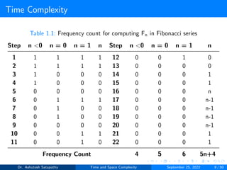
  • 9. Time Complexity Table 1.1: Frequency count for computing Fn in Fibonacci series Step n <0 n = 0 n = 1 n Step n <0 n = 0 n = 1 n 1 1 1 1 1 12 0 0 1 0 2 1 1 1 1 13 0 0 0 0 3 1 0 0 0 14 0 0 0 1 4 1 0 0 0 15 0 0 0 1 5 0 0 0 0 16 0 0 0 n 6 0 1 1 1 17 0 0 0 n-1 7 0 1 0 0 18 0 0 0 n-1 8 0 1 0 0 19 0 0 0 n-1 9 0 0 0 0 20 0 0 0 n-1 10 0 0 1 1 21 0 0 0 1 11 0 0 1 0 22 0 0 0 1 Frequency Count 4 5 6 5n+4 Dr. Ashutosh Satapathy Time and Space Complexity September 25, 2022 9 / 50
  • 10. Outline 1 Algorithm Analysis Time and Space Complexity Time Complexity Space Complexity 2 Asymptotic Notation Basics Asymptote Big-Oh notation Big Omega notation Little-Oh notation Little-Omega notation Theta notation Limit Definition 3 Complexity Analysis Growth of Functions Types of Time Complexities Time Complexity Analysis Space Complexity Analysis Dr. Ashutosh Satapathy Time and Space Complexity September 25, 2022 10 / 50
  • 11. Space Complexity The space needed by a program is the sum of the following components. Fixed space requirement: The component refers to space requirement that do not depend on the number and size of the program’s inputs and outputs. The fixed requirements include the instruction space (space needed to store the code), space for simple variables, fixed size structured variable and constants. Variable space requirement: This component consists of the space needed by structured variables whose size depends on the particular instance i, of the problem being solved. It also includes the additional space required when a function uses recursion. The space requirement S(P) of an algorithm P may therefore be written as S(P) = c + SP, where c and SP are the constant and instance characteristics, respectively. First, we need to determine which instance characteristics to use for a give problem to reduce the space requirements. Dr. Ashutosh Satapathy Time and Space Complexity September 25, 2022 11 / 50
  • 12. Space Complexity Algorithm 2 Square of the given Number 1: procedure getsquare(n) 2: return n*n 3: end procedure We can solve the problem without consuming any extra space, hence the space complexity is constant. Dr. Ashutosh Satapathy Time and Space Complexity September 25, 2022 12 / 50
  • 13. Space Complexity Algorithm 3 Sum of array elements 1: procedure calculate sum(A, n) 2: sum ← 0 3: for i ← 0 to n − 1 do 4: sum ← sum + A[i] 5: end for 6: end procedure n, sum and i take constant sum of 3 units, but the variable A is an array, it’s space consumption increases with the increase of input size n. Dr. Ashutosh Satapathy Time and Space Complexity September 25, 2022 13 / 50
  • 14. Outline 1 Algorithm Analysis Time and Space Complexity Time Complexity Space Complexity 2 Asymptotic Notation Basics Asymptote Big-Oh notation Big Omega notation Little-Oh notation Little-Omega notation Theta notation Limit Definition 3 Complexity Analysis Growth of Functions Types of Time Complexities Time Complexity Analysis Space Complexity Analysis Dr. Ashutosh Satapathy Time and Space Complexity September 25, 2022 14 / 50
  • 15. Basics The main idea of asymptotic analysis is to have a measure of efficiency of algorithms that doesn’t depend on machine specific constants. Asymptotic analysis of an algorithm refers to defining the mathematical boundation/framing of its run-time performance. It doesn’t require algorithms to be implemented and time taken by programs to be compared. Asymptotic notations are mathematical tools to represent time complexity of algorithms for asymptotic analysis. Dr. Ashutosh Satapathy Time and Space Complexity September 25, 2022 15 / 50
  • 16. Outline 1 Algorithm Analysis Time and Space Complexity Time Complexity Space Complexity 2 Asymptotic Notation Basics Asymptote Big-Oh notation Big Omega notation Little-Oh notation Little-Omega notation Theta notation Limit Definition 3 Complexity Analysis Growth of Functions Types of Time Complexities Time Complexity Analysis Space Complexity Analysis Dr. Ashutosh Satapathy Time and Space Complexity September 25, 2022 16 / 50
  • 17. Asymptote A ’Line’ that continually approaches a given curve but does not meet it at any finite distance. The term asymptotic means approaching a value or curve arbitrarily closely (i.e., as some sort of limit is taken). A line or a curve A that is asymptotic to given curve C is called the asymptote of C. Figure 2.1: Asymptote of curve f(x) Dr. Ashutosh Satapathy Time and Space Complexity September 25, 2022 17 / 50
  • 18. Outline 1 Algorithm Analysis Time and Space Complexity Time Complexity Space Complexity 2 Asymptotic Notation Basics Asymptote Big-Oh notation Big Omega notation Little-Oh notation Little-Omega notation Theta notation Limit Definition 3 Complexity Analysis Growth of Functions Types of Time Complexities Time Complexity Analysis Space Complexity Analysis Dr. Ashutosh Satapathy Time and Space Complexity September 25, 2022 18 / 50
  • 19. O (Big-Oh) notation Big-Oh is used as a tight upper-bound on the growth of an algorithm’s effort (this effort is described by the function f(n)). Let f(n) and g(n) be functions that map positive integers to positive real numbers. We say that f(n) is O(g(n)) or f(n) ∈ O(g(n)), if there exists a real constant c > 0 and there exists an integer constant n0 ≥ 1 such that f(n) ≤ cg(n) for every integer n ≥ n0. In other words O(g(n)) = {f(n): there exist positive constants c and n0 such that 0 ≤ f(n) ≤ cg(n) for all n ≥ n0} Figure 2.2: f(n) ∈ O(g(n)) Dr. Ashutosh Satapathy Time and Space Complexity September 25, 2022 19 / 50
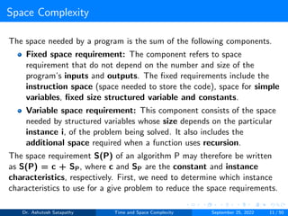
  • 20. O (Big-Oh) notation Question 1: Consider the function f(n) = 6n+ 135. Clearly. f(n) is non-negative for all integers n ≥ 0. We wish to show that f(n)=O(n2). According to the Big-oh definition, in order to show this we need to find an integer n0, and a constant c > 0 such that for all integers, n ≥ n0, f(n) = c(n2) Answer: Suppose we choose c = 1, and f(n) = cn2. ⇒ 6n+135 = cn2 = n2 [Since c = 1] n2-6n-135 = 0 ⇒ (n-15)(n+9) = 0 Since (n+9) > 0 for all values n ≥ 0, we conclude that (n-15) = 0 ⇒ n0 = 15 for c = 1 For c = 2, n0 = (6 + √ 1116)/4 ≈ 9.9 For c = 4, n0 = (6 + √ 2196)/8 ≈ 6.7 Dr. Ashutosh Satapathy Time and Space Complexity September 25, 2022 20 / 50
  • 21. Outline 1 Algorithm Analysis Time and Space Complexity Time Complexity Space Complexity 2 Asymptotic Notation Basics Asymptote Big-Oh notation Big Omega notation Little-Oh notation Little-Omega notation Theta notation Limit Definition 3 Complexity Analysis Growth of Functions Types of Time Complexities Time Complexity Analysis Space Complexity Analysis Dr. Ashutosh Satapathy Time and Space Complexity September 25, 2022 21 / 50
  • 22. Ω (Big-Omega) notation Big-Omega (Ω) is the tight lower bound notation. Let f(n) and g(n) be functions that map positive integers to positive real numbers. We say that f(n) is Ω(g(n)) or f(n) ∈ Ω(g(n)) if there exists a real constant c > 0 and there exists an integer constant n0 ≥ 1 such that f(n) ≥ cg(n) for every integer n ≥ n0. In other words Ω(g(n)) = {f(n): there exist positive constants c and n0 such that 0 ≤ cg(n) ≤ f(n) for all n ≥ n0}. Figure 2.3: f(n) ∈ Ω(g(n)) Dr. Ashutosh Satapathy Time and Space Complexity September 25, 2022 22 / 50
  • 23. Ω (Big-Omega) notation Question 2: Consider the function f(n)= 3n2-24n+72. Clearly f(n) is non-negative for all integers n ≥ 0. We wish to show that f(n) = Ω(n2). According to the big-omega definition, in order to show this we need to find an integer n0,and a constant c > 0 such that for all integers n = n0, f(n) = cn2. Answer: Suppose we choosc c = 1, Then f(n) = cn2 ⇒ 3n2-24n+72 = n2 ⇒ 2n2-24n+72 = 0 ⇒ 2(n-6)2 = 0 Since (n-6)2 = 0, we conclude that n0 = 6. So we have that for c = 1 and n ≥ 6, f(n) = cn2. Hence f(n) = Ω(n2). Dr. Ashutosh Satapathy Time and Space Complexity September 25, 2022 23 / 50
  • 24. Outline 1 Algorithm Analysis Time and Space Complexity Time Complexity Space Complexity 2 Asymptotic Notation Basics Asymptote Big-Oh notation Big Omega notation Little-Oh notation Little-Omega notation Theta notation Limit Definition 3 Complexity Analysis Growth of Functions Types of Time Complexities Time Complexity Analysis Space Complexity Analysis Dr. Ashutosh Satapathy Time and Space Complexity September 25, 2022 24 / 50
  • 25. o (Little-Oh) notation Little-oh (o) is used as a loose upper-bound on the growth of an algorithm’s effort (this effort is described by the function f(n)). Let f(n) and g(n) be functions that map positive integers to positive real numbers. We say that f(n) is o(g(n)) or f(n) ∈ o(g(n)) if for any real constant c > 0, there exists an integer constant n0 ≥ 1 such that f(n) < cg(n) for every integer n ≥ n0. In other words o(g(n)) = {f(n): there exist positive constants c and n0 such that 0 ≤ f(n) < cg(n) for all n ≥ n0}. Figure 2.4: f(n) ∈ o(g(n)) Dr. Ashutosh Satapathy Time and Space Complexity September 25, 2022 25 / 50
  • 26. Outline 1 Algorithm Analysis Time and Space Complexity Time Complexity Space Complexity 2 Asymptotic Notation Basics Asymptote Big-Oh notation Big Omega notation Little-Oh notation Little-Omega notation Theta notation Limit Definition 3 Complexity Analysis Growth of Functions Types of Time Complexities Time Complexity Analysis Space Complexity Analysis Dr. Ashutosh Satapathy Time and Space Complexity September 25, 2022 26 / 50
  • 27. ω (Little-Omega) notation Little Omega (ω) is used as a loose lower-bound on the growth of an algorithm’s effort (this effort is described by the function f(n)). Let f(n) and g(n) be functions that map positive integers to positive real numbers. We say that f(n) is ω(g(n)) or f(n) ∈ ω(g(n)) if for any real constant c > 0, there exists an integer constant n0 ≥ 1 such that f(n) > cg(n) for every integer n ≥ n0. In other words ω(g(n)) = {f(n): there exist positive constants c and n0 such that 0 ≤ cg(n) < f(n) for all n ≥ n0}. Figure 2.5: f(n) ∈ ω(g(n)) Dr. Ashutosh Satapathy Time and Space Complexity September 25, 2022 27 / 50
  • 28. Outline 1 Algorithm Analysis Time and Space Complexity Time Complexity Space Complexity 2 Asymptotic Notation Basics Asymptote Big-Oh notation Big Omega notation Little-Oh notation Little-Omega notation Theta notation Limit Definition 3 Complexity Analysis Growth of Functions Types of Time Complexities Time Complexity Analysis Space Complexity Analysis Dr. Ashutosh Satapathy Time and Space Complexity September 25, 2022 28 / 50
  • 29. θ (Theta) notation Let f(n) and g(n) be functions that map positive integers to positive real numbers. We say that f(n) is θ(g(n)) or f(n) ∈ θ(g(n)) if and only if f(n) ∈ O(g(n)) and f(n) ∈ Ω(g(n)) θ(g(n)) = {f(n): there exist positive constants c1, c2 and n0 such that 0 ≤ c1g(n) ≤ f(n) ≤ c2g(n) for all n ≥ n0} Figure 2.6: f(n) ∈ θ(g(n)) Dr. Ashutosh Satapathy Time and Space Complexity September 25, 2022 29 / 50
  • 30. Outline 1 Algorithm Analysis Time and Space Complexity Time Complexity Space Complexity 2 Asymptotic Notation Basics Asymptote Big-Oh notation Big Omega notation Little-Oh notation Little-Omega notation Theta notation Limit Definition 3 Complexity Analysis Growth of Functions Types of Time Complexities Time Complexity Analysis Space Complexity Analysis Dr. Ashutosh Satapathy Time and Space Complexity September 25, 2022 30 / 50
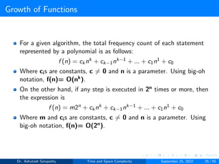
  • 31. Limit Definition 1 if f (n) ∈ O(g(n)) then limn→∞ f (n) g(n) ∈ [0, ∞) 2 if f (n) ∈ o(g(n)) then limn→∞ f (n) g(n) = 0 3 if f (n) ∈ Ω(g(n)) then limn→∞ f (n) g(n) ∈ (0, ∞] 4 if f (n) ∈ ω(g(n)) then limn→∞ f (n) g(n) = ∞ 5 if f (n) ∈ θ(g(n)) then limn→∞ f (n) g(n) ∈ (0, ∞) Examples 1. n2 − 2n + 5 ∈ O(n3) ⇔ limn→∞ n2−2n+5 n3 = limn→∞ 1 n − 2 n2 + 5 n3 = 0 2. n2 + 1 ∈ Ω(n) ⇔ limn→∞ n2+1 n = ∞ 3. n2 + 3n + 4 ∈ θ(n2) ⇔ limn→∞ n2+3n+4 n2 = limn→∞(1 + 3 n + 4 n2 ) = 1 4. 7n + 8 ∈ o(n2) ⇔ limn→∞ 7n+8 n2 = limn→∞(7 n + 8 n2 ) = 0 5. 4n + 6 ∈ ω(1) ⇔ limn→∞ 4n+6 1 = ∞ Dr. Ashutosh Satapathy Time and Space Complexity September 25, 2022 31 / 50
  • 32. Outline 1 Algorithm Analysis Time and Space Complexity Time Complexity Space Complexity 2 Asymptotic Notation Basics Asymptote Big-Oh notation Big Omega notation Little-Oh notation Little-Omega notation Theta notation Limit Definition 3 Complexity Analysis Growth of Functions Types of Time Complexities Time Complexity Analysis Space Complexity Analysis Dr. Ashutosh Satapathy Time and Space Complexity September 25, 2022 32 / 50
  • 33. Growth of Functions The order of growth of the running time of an algorithm gives a simple characterization of the algorithm’s efficiency and also allows us to compare the relative performance of alternative algorithms. We are concerned with how the running time of an algorithm increases with the size of the input increases. We write O(1) to mean a computing time which is a constant. O(n) is called linear, O(n2) is called quadratic, O(n3) is called cubic and O(2n) is called exponential. If an algorithm takes time O(log2n) it is faster, for sufficiently large n, than if it had taken O(n). Similarly, O(nlog2n) is better than O(n2) but not as good as O(n). It we have two algorithms which perform the same task, and the first has a computing time, which is O(n) and the second O(n2), then we will usually take the first as superior. Dr. Ashutosh Satapathy Time and Space Complexity September 25, 2022 33 / 50
  • 34. Growth of Functions Table 3.1: The cumulative frequency count of instructions of two algorithms. n 10n n2/2 1 10 0.5 5 50 12.5 10 100 50 15 150 112.5 20 200 200 25 250 312.5 30 300 450 For n≤20, algorithm two had a smaller computing time, but once past that point, algorithm one became better. This shows why we chose the algorithm with the smaller order of magnitude. Dr. Ashutosh Satapathy Time and Space Complexity September 25, 2022 34 / 50
  • 35. Growth of Functions For a given algorithm, the total frequency count of each statement represented by a polynomial is as follows: f (n) = cknk + ck−1nk−1 + ... + c1n1 + c0 Where cis are constants, c ̸= 0 and n is a parameter. Using big-oh notation, f(n)= O(nk). On the other hand, if any step is executed in 2n times or more, then the expression is f (n) = m2n + cknk + ck−1nk−1 + ... + c1n1 + c0 Where m and cis are constants, c ̸= 0 and n is a parameter. Using big-oh notation, f(n)= O(2n). Dr. Ashutosh Satapathy Time and Space Complexity September 25, 2022 35 / 50
  • 36. Growth of Functions Table 3.2: Values of computing functions log2n n nlog2n n2 n3 2n n! 0 1 0 1 1 2 1 1 2 2 4 8 4 2 2 4 8 16 64 16 24 3 8 24 64 512 256 40,320 4 16 64 256 4096 65,536 20,922,789,888,000 5 32 160 1024 32768 2,147,483,648 2.631308369E+35 Another valid performance measure of an algorithm is space. Often, one can trade space for time, getting a faster algorithm while using more space. Dr. Ashutosh Satapathy Time and Space Complexity September 25, 2022 36 / 50
  • 37. Outline 1 Algorithm Analysis Time and Space Complexity Time Complexity Space Complexity 2 Asymptotic Notation Basics Asymptote Big-Oh notation Big Omega notation Little-Oh notation Little-Omega notation Theta notation Limit Definition 3 Complexity Analysis Growth of Functions Types of Time Complexities Time Complexity Analysis Space Complexity Analysis Dr. Ashutosh Satapathy Time and Space Complexity September 25, 2022 37 / 50
  • 38. Types of Time Complexities Time complexity usually depends on the size of the algorithm and input. The best-case time complexity of an algorithm is a measure of the minimum time that the algorithm will require for an input of size n. The worst-case time complexity of an algorithm is a measure of the maximum time that the algorithm will require for an input of size n. After knowing the worst-case time complexity, we can guarantee that the algorithm will never take more than this time. The time that an algorithm will require to execute a typical input data of size n is known as average-case time complexity. We can say that the value that is obtained by averaging the running time of an algorithm for all possible inputs of size n can determine average-case time complexity. Dr. Ashutosh Satapathy Time and Space Complexity September 25, 2022 38 / 50
  • 39. Outline 1 Algorithm Analysis Time and Space Complexity Time Complexity Space Complexity 2 Asymptotic Notation Basics Asymptote Big-Oh notation Big Omega notation Little-Oh notation Little-Omega notation Theta notation Limit Definition 3 Complexity Analysis Growth of Functions Types of Time Complexities Time Complexity Analysis Space Complexity Analysis Dr. Ashutosh Satapathy Time and Space Complexity September 25, 2022 39 / 50
  • 40. Rules for Complexity Analysis Rule 1: Sequence The worst case running time of a sequence of C statements such as statement 1; statement 2; statement 3; . . . statement m; is O(max(T1(n), T2(n), ...Tm(n))), where running time of Si, the ith statement in the sequence, is O(Ti(n)) Dr. Ashutosh Satapathy Time and Space Complexity September 25, 2022 40 / 50
  • 41. Rules for Complexity Analysis Rule 2: Iteration The worst case running time of a C for loop such as for(statement 1; statement 2; statement 3) statement 4 is O(max(T1(n), T2(n)(I(n)+1), T3(n)I(n), T4(n)I(n))), where the running time of statement Si is O(Ti(n)), for i=1,2,3 and 4, and I(n) is the number of iterations executed in the worst case. Rule 2: Selection The worst care running time of a C if- else such as if (statement 1) statement 2; else statement 3; is O(max(T1(n), T2(n), T3(n))), where the running time of statement Si, is O(Ti(n)), for i= 1,2 and 3. Dr. Ashutosh Satapathy Time and Space Complexity September 25, 2022 41 / 50
  • 42. Rules for Complexity Analysis Algorithm 4 Prefix-sum 1: procedure prefix-sum(A, n) 2: for i ← n − 1 to 0 do 3: sum ← 0 4: for j ← 0 to i do 5: sum ← sum + A[j] 6: end for 7: A[i] ← sum 8: end for 9: end procedure Dr. Ashutosh Satapathy Time and Space Complexity September 25, 2022 42 / 50
  • 43. Rules for Complexity Analysis Table 3.3: Time Complexity calculation of Prefix-sum algorithm Statement Frequency Count Time 1 1 O(1) 2 n+1 O(n) 3 n O(n) 4 (n+1) + n + ....+ 2 O(n2) 5 n + (n-1) + ...+ 1 O(n2) 6 n + (n-1) + ...+ 1 O(n2) 7 n O(n) 8 n O(n) 9 1 O(1) f(n) (n+1)(n+2)/2 + n(n+1) + 4n + 2 O(n2) Dr. Ashutosh Satapathy Time and Space Complexity September 25, 2022 43 / 50
  • 44. Outline 1 Algorithm Analysis Time and Space Complexity Time Complexity Space Complexity 2 Asymptotic Notation Basics Asymptote Big-Oh notation Big Omega notation Little-Oh notation Little-Omega notation Theta notation Limit Definition 3 Complexity Analysis Growth of Functions Types of Time Complexities Time Complexity Analysis Space Complexity Analysis Dr. Ashutosh Satapathy Time and Space Complexity September 25, 2022 44 / 50
  • 45. Space Complexity Analysis Example 1 In Algorithm 2, the variable n occupies a constant 4 Bytes of memory. The function call and return statement come under the auxiliary space and let’s assume 4 Bytes all together. The total space complexity is 8 Bytes. Algorithm 2 has a space complexity of O(1). Example 2 In Algorithm 3, the variables n, sum, and i occupy a constant 12 Bytes of memory. The function call, initialisation of the for loop and write function all come under the auxiliary space and let’s assume 4 Bytes all together. The total space complexity is 4n + 16 Bytes. Algorithm 3 has a space complexity of O(n). Dr. Ashutosh Satapathy Time and Space Complexity September 25, 2022 45 / 50
  • 46. Space Complexity Analysis Algorithm 5 Factorial of a number 1: procedure factorial(n) 2: fact ← 1 3: for i ← 1 to n do 4: fact ← fact + i 5: end for 6: return fact 7: end procedure The variables n, fact, and i occupy a constant 12 Bytes of memory. The function call, initializing the for loop and return statement all come under the auxiliary space and let’s assume 4 Bytes all together. The total space complexity is 16 Bytes. Algorithm 5 has a space complexity of O(1). Dr. Ashutosh Satapathy Time and Space Complexity September 25, 2022 46 / 50
  • 47. Space Complexity Analysis Algorithm 6 Recursive: Factorial of a number 1: procedure factorial(n) 2: if (n ≤ 1) then 3: return 1 4: else 5: return n ∗ FACTORIAL(n − 1) 6: end if 7: end procedure The variable n occupies a constant 4 Bytes of memory. The function call, if and else conditions and return statement all come under the auxiliary space and let’s assume 4 Bytes all together. The total space complexity is 4n+4 Bytes. Algorithm 6 has a space complexity of O(n). Dr. Ashutosh Satapathy Time and Space Complexity September 25, 2022 47 / 50
  • 48. Space Complexity Analysis Algorithm 7 Summation of two numbers 1: procedure addition(a, b) 2: c ← a + b 3: write c 4: end procedure The variables a, b and c occupy a constant 12 Bytes of memory. The function call, if and else conditions and write function all come under the auxiliary space and let’s assume 4 Bytes all together. The total space complexity is 16 Bytes. Algorithm 7 has a space complexity of O(1). Dr. Ashutosh Satapathy Time and Space Complexity September 25, 2022 48 / 50
  • 49. Summary Here, we have discussed Introduction to time and space complexity. Different types of asymptotic notations and their limit definitions. Growth of functions and types of time complexities. Time and space complexity analysis of various algorithms. Dr. Ashutosh Satapathy Time and Space Complexity September 25, 2022 49 / 50
  • 50. For Further Reading I H. Sahni and A. Freed. Fundamentals of Data Structures in C (2nd edition). Universities Press, 2008. A. K. Rath and A. K. Jagadev. Data Structures Using C (2nd edition). Scitech Publications, 2011. Dr. Ashutosh Satapathy Time and Space Complexity September 25, 2022 50 / 50