Time Series Analysis:Complete
Guide from Statistics to
Deep Learning
A comprehensive exploration of techniques, models, and
applications for analyzing temporal data patterns and making
accurate forecasts
Presenter: Data Science Expert
August 2025
Made with
Genspark
2.
Table of Contents
Thispresentation provides a comprehensive overview of
time series analysis from fundamental statistical methods
to cutting- edge deep learning techniques. Progression of techniques from statistical methods to advanced deep
learning
In This Presentation
Introduction to Time Series Analysis - definitions,
importance, and applications
Time Series Components - trend, seasonality, cycle, and
noise
Statistical Techniques - stationarity, transformations,
and decomposition
Classical Models - ARIMA, SARIMA, and exponential
smoothing Advanced Models - VAR, GARCH, and state
space models
Machine Learning and Deep Learning Approaches - RNN,
LSTM, and transformers
Made with Genspark
3.
What is TimeSeries Analysis?
A time series decomposed into its components: trend, seasonality, and
random variations
Definition & Importance
Time series analysis is the study of data points collected
over time at regular intervals, with the goal of
identifying patterns, trends, and making predictions
about future values.
Key Characteristics
Temporal Ordering: Data points have a chronological
sequence that matters
Autocorrelation: Observations are not independent; they
relate to previous values
Multiple Components: Often contains trend, seasonality,
cyclical patterns, and random noise
Specialized Methods: Requires dedicated statistical and
machine learning techniques
Domain-Specific: Analysis approaches vary based on the
field (finance, economics, healthcare, etc.)
4.
Why Analyze TimeSeries Data?
Organizations that effectively analyze time series data gain
35% better forecast accuracy and reduce operational costs
by up to 25% through improved resource allocation and
risk management.
Business value of time series analysis across
industries
Key Goals and Business Value
Forecasting: Predict future values to support proactive
decision- making and resource planning
Pattern Recognition: Identify hidden patterns,
seasonality, and anomalies in historical data
Causal Analysis: Understand what factors influence changes
over time
Risk Management: Quantify uncertainty and prepare for
potential volatility
Performance Monitoring: Track KPIs over time and
detect deviations from expected behavior
5.
How Time SeriesAnalysis Differs from Other Analyses
These unique properties of time series data
necessitate specialized analytical approaches that
account for temporal dependencies and patterns.
Key differences between time series analysis and standard statistical
analysis
Unique Characteristics
Temporal Ordering: The sequence of observations
matters fundamentally, unlike cross-sectional data
where ordering is arbitrary
Dependence Structure: Observations are not
independent; current values depend on past values
Autocorrelation: Values are correlated with their own
previous values at various lags
Non-stationarity: Statistical properties (mean, variance)
often change over time
Specialized Methods: Requires specific techniques like
ARIMA, decomposition, and spectral analysis
6.
1
Section 1: TimeSeries
Fundamentals
Understanding the
basics
An introduction to core concepts,
components, and properties of time series
data that form the foundation for all
analysis techniques.
Made with Genspark
Time Series Analysis: Complete Guide from Statistics to Deep
Learning
7.
What is aTime Series? (Detailed)
Practical Example
Consider daily stock prices for Company XYZ over one year:
import pandas as pd
import matplotlib.pyplot as plt
# Load stock price data
stock_data = pd.read_csv('xyz_stock.csv') stock_data['Date'] =
pd.to_datetime(stock_data['Date']) stock_data.set_index('Date',
inplace=True)
# Plot the time series plt.figure(figsize=(10, 6))
plt.plot(stock_data['Close']) plt.title('XYZ Stock Price
(2023-2024)') plt.ylabel('Price ($)')
plt.grid(True)
plt.show()
Definition & Concepts
A time series is a sequence of data points collected or recorded at
specific time intervals. Unlike regular data, the temporal ordering is
crucial as it captures how values change over time.
Understanding the temporal dependencies between
observations is what makes time series analysis unique
compared to other statistical methods.
Values are ordered chronologically
Intervals are typically uniform (hourly, daily,
monthly) Observations are dependent on
previous values
Used for forecasting future values based on
historical patterns
8.
Core Properties ofTime Series
Understanding these core properties is essential for
choosing appropriate preprocessing techniques,
selecting the right models, and accurately interpreting
results in time series analysis.
Illustration of temporal ordering and lag relationships in a time
series
Key Characteristics
Temporal Ordering: Data points are sequentially
ordered by timestamps, creating a natural progression
that cannot be randomly shuffled like other data types
Temporal Dependence: Future values typically depend
on past observations, creating autocorrelation patterns
that are crucial for forecasting
Lag Relationships: The influence of past values (lags) on
current values, where observations at t-1, t-2, etc., impact
the value at time t
Granularity: The time interval between observations
(hourly, daily, monthly) that affects data patterns and
modeling approaches
9.
Components of TimeSeries: Level, T
rend, Seasonality
Key Components of Time Series
Data
Level
The baseline value or the average value around which the
time series fluctuates. Represents the underlying value of
the series when other components are removed.
Trend
Long-term upward or downward movement in the data.
Shows the general direction in which the time series is
moving over an extended period.
Seasonality
Regular and predictable patterns that repeat over fixed
periods (daily, weekly, monthly, quarterly). Caused by
seasonal factors like weather
, holidays, or business cycles.
Understanding these components is crucial for effective
time series modeling and forecasting. Models can be
designed to capture each component specifically. Decomposition of a time series into its basic
components
10.
Cyclical Patterns andNoise
WHY it matters: Distinguishing between cyclical patterns
and noise is crucial for accurate forecasting. Cycles
represent real patterns that can be modeled, while noise
must be filtered out.
Cyclical pattern in economic data (business
cycle)
Random noise component in time
series
Understanding Time Series Components
Cyclical Patterns: Fluctuations that occur without
fixed frequencies, unlike seasonal patterns
Key Characteristics: Non-fixed periodicity, often spans
multiple years (business cycles, economic fluctuations)
Example: Economic expansions and contractions,
financial market cycles
Noise Component: Random, irregular fluctuations in time
series data
Importance of Noise: Represents unexplained variation
that can't be attributed to trend, seasonality, or cycles
11.
Types of TimeSeries Data
Univariate vs Multivariate
Time series data can be categorized based on the number of
variables measured at each time point. Understanding these
types is critical for selecting appropriate analysis methods.
The complexity and richness of insights increases with the
number of variables tracked over time.
Univariate Multivariate
Single variable
tracked over time
Multiple variables tracked simultaneously
Examples: Daily
temperature, stock
price
Examples: Weather data (temp,
humidity, pressure), financial
indicators
Simpler
analysis
techniques
Captures relationships between variables
Practical Examples
Consider these two approaches to analyzing retail data:
import pandas as pd
import matplotlib.pyplot as plt
# Load retail dataset
retail_data = pd.read_csv('retail_sales.csv') retail_data['Date'] =
pd.to_datetime(retail_data['Date'])
# Univariate approach - just sales univariate_series =
retail_data.set_index('Date') ['Sales']
# Multivariate approach - sales, customer count, and promotions
multivariate_series = retail_data.set_index('Date') [['Sales',
'CustomerCount', 'PromotionExpense']]
# Correlation analysis (only possible with multivariate)
correlation_matrix = multivariate_series.corr() print(correlation_matrix)
Univariate models focus on patterns within a single sequence
Multivariate analysis reveals relationships and
12.
Stationarity in TimeSeries
What is
Stationarity?
When your time series isn't stationary, transformations
like differencing, logarithmic transformation, or Box-Cox
Comparison of stationary vs. non-stationary time series. The stationary series
(blue) maintains consistent statistical properties over time, while the non-
A time series is stationary when its statistical properties do not
change over time. Specifically, this means:
Constant mean (no trend)
Constant variance (homoscedasticity)
Constant autocorrelation structure (pattern of
dependence doesn't change)
Why is Stationarity Important?
Most statistical forecasting methods assume stationarity
Makes forecasting more reliable as patterns remain
consistent Simplifies mathematical models and improves
interpretability Easier to detect genuine patterns vs
random fluctuations
13.
Examples of Stationaryvs. Non-Stationary Series
Real-World Examples
Example 1: Stock Prices (Non-
Stationary)
Google stock price - exhibits clear upward trend (non-
stationary)
After Differencing
Example 2: Stock Returns (Stationary)
Understanding Stationarity
A stationary time series has statistical properties that do not
change over time - specifically constant mean, variance, and
autocorrelation structure.
Most statistical time series models (like ARIMA)
require stationarity to make valid predictions!
Stationary series: White noise, differenced stock returns,
residuals after removing trend/seasonality
Non-stationary series: Stock prices, GDP
, temperature
readings with seasonal patterns
We can transform non-stationary series to
stationary using differencing, detrending, or seasonal
adjustment
Statistical tests like ADF, KPSS, and Phillips-Perron help
determine stationarity
14.
Applications & UseCases
Time series analysis provides valuable insights across Relative adoption of time series analysis techniques by
industry
Time Series Analysis Across Industries
Finance: Stock price prediction, portfolio optimization, risk
management, algorithmic trading, and market volatility
analysis
Retail & E-commerce: Demand forecasting, inventory
management, sales prediction, seasonal pattern
identification, and pricing optimization
Healthcare: Patient monitoring, disease progression
tracking, epidemic outbreak prediction, and hospital
resource planning
Energy & Utilities: Load forecasting, renewable energy
production prediction, consumption pattern analysis, and
smart grid optimization
Manufacturing: Predictive maintenance, production
planning, supply chain optimization, and quality control
Environment & Climate: Weather forecasting, climate
change analysis, natural disaster prediction, and
ecological monitoring
15.
2
Section 2: Data
Preprocessing
&
Exploration
Preparingand understanding
your
dat
a
Essential techniques for cleaning,
transforming, and exploring time series
data to ensure accurate analysis and
modeling results.
Made with Genspark
Time Series Analysis: Complete Guide from Statistics to Deep
Learning
16.
Checking Stationarity: How& Why
Statistical Tests for Stationarity
Stationarity is critical for time series modeling because many
techniques assume statistical properties remain constant over time.
Rather than relying on visual inspection alone, we use formal
statistical tests to confirm stationarity.
Why test for stationarity? Non-stationary data can lead to
spurious regressions and unreliable forecasts in traditional time
series models.
Tes
t
Null
Hypothesi
s
Interpretati
on
AD
F
(Augmented
Dickey- Fuller)
Series has
a unit root
(non-
stationary)
p-value < 0.05: Reject
null hypothesis
(stationary)
KPSS
(Kwiatkowski-
Phillips- Schmidt-
Shin)
Series is
stationar
y
p-value < 0.05: Reject null
hypothesis (non-
stationary)
PP
Series has
a unit root p-value < 0.05: Reject
Practical Implementation
Using Python's statsmodels to test for stationarity:
import pandas as pd
import numpy as np
from statsmodels.tsa.stattools import adfuller, kpss import
matplotlib.pyplot as plt
# Example time series (non-stationary with trend)
np.random.seed(42)
ts = pd.Series(np.cumsum(np.random.normal(0.1, 1, 100)))
# Run ADF test adf_result =
adfuller(ts)
print(f'ADF Statistic: {adf_result[0]:.4f}') print(f'p-value:
{adf_result[1]:.4f}') print('Critical Values:')
for key, value in adf_result[4].items():
print(f' {key}: {value:.4f}')
# Run KPSS test kpss_result
= kpss(ts)
print(f'KPSS Statistic: {kpss_result[0]:.4f}') print(f'p-value:
{kpss_result[1]:.4f}')
17.
Transformations for Time
Series
Transformatio
n
Whento Use Why It Works
Log Transform
Data with
exponential
growth or
multiplicative
patterns
Reduces exponential trends
to linear; stabilizes variance
when SD proportional to
mean
Box-Cox
When simple
log transform
isn't optimal
Family of power
transformations that
finds optimal parameter
(λ) to normalize data
Series with trend
Removes trend (1st diff)
and seasonality (seasonal
Why Transform Time Series Data?
Stabilize variance - Make data more consistent across
time Achieve stationarity - Essential for many
forecasting models Normalize distribution - Make data
more symmetrical Remove trend & seasonality -
Isolate the underlying patterns
18.
Handling Missing Values& Outliers
Practical Example
Let's examine how to handle missing values and outliers in monthly
sales data:
import pandas as pd
import numpy as np
import matplotlib.pyplot
as plt
# Load time series with missing values and outliers sales =
pd.read_csv('monthly_sales.csv', parse_dates= ['date'])
# 1. Handle missing values with interpolation sales_clean =
sales.copy() sales_clean['value'] =
sales_clean['value'].interpolate(method='time')
# 2. Detect and handle outliers with IQR method Q1 =
sales_clean['value'].quantile(0.25)
Q3 = sales_clean['value'].quantile(0.75)
IQR = Q3 - Q1
lower_bound = Q1 - 1.5 * IQR
upper_bound = Q3 + 1.5 * IQR
# Replace outliers with median of neighboring points mask =
Why It Matters
Time series data often contains missing values and outliers that
can significantly distort analysis and forecasting models. Properly
handling these anomalies is crucial for accurate modeling.
Ignoring missing values or outliers can lead to biased
parameter estimates, unreliable forecasts, and misleading
insights about the underlying patterns.
Missing Value Techniques
Forward/Backward Fill - Propagate last known value
forward or first known value backward
Interpolation - Linear
, spline, or time-weighted methods
to estimate missing points
Statistical Imputation - Replace with mean, median, or
model-based estimates
Outlier Detection & Treatment
IQR Method - Identify points beyond 1.5×IQR from
19.
Resampling and FrequencyAdjustment
In Python: df.resample('M').mean() - Resample to
Visual comparison of original daily data vs. weekly and monthly
resampling
Why Resample Time Series Data?
Change analysis granularity - Aggregate daily
data to weekly/monthly for high-level trends
Reduce noise - Lower frequencies often smooth out
short-term fluctuations
Match different data sources - Align data collected at
different frequencies
Computational efficiency - Reduce dataset size for
faster processing
How to Resample?
Upsampling - Increase frequency (e.g., monthly → daily);
requires interpolation
Downsampling - Decrease frequency (e.g., daily →
monthly); requires aggregation
20.
Visualizing Time Series
Choosingthe right visualization depends on what aspect
of the time series you want to analyze. Combining
Different visualization methods applied to the same time series
data
Common Visualization Methods
Line plots: Most basic visualization showing evolution over
time; reveals overall trends, patterns, and outliers
Seasonal plots: Overlays same seasons from different
cycles; highlights seasonal patterns and variations
between cycles
Lag plots: Shows relationship between an observation and
its lagged value; useful for identifying autocorrelation and
non-linear patterns
ACF/PACF plots: Displays correlations between the series
and its lags; reveals dependencies and helps with model
selection
Heatmaps: Color-coded grid visualization; effective for
multiple time series or displaying cyclical patterns by
hour/day/month
Decomposition plots: Breaks down series into trend,
seasonal, and residual components; helps understand
underlying patterns
21.
Seasonal Decomposition (STL,Classical)
STL Decomposition
Example
import pandas as pd
import matplotlib.pyplot as plt
from statsmodels.tsa.seasonal import seasonal_decompose
# Monthly airline passenger data
airline = pd.read_csv('airline_passengers.csv') airline['Month'] =
pd.to_datetime(airline['Month']) airline.set_index('Month',
inplace=True)
# Apply STL decomposition
decomposition = seasonal_decompose(airline['Passengers'],
model='multiplicative',
period=12)
# Plot the decomposed components fig
= decomposition.plot() plt.tight_layout()
plt.show()
What is Seasonal Decomposition?
Seasonal decomposition is a technique that breaks down a time
series into its constituent components: trend, seasonality, and
residuals. This helps in better understanding the underlying patterns
and improving forecasting accuracy.
Decomposition reveals hidden patterns that might not be
visible in the original series, making it easier to model each
component separately.
Two Main Approaches:
Classical Decomposition: Simple approach that assumes
constant seasonal component; can be additive or
multiplicative
STL (Seasonal-Trend decomposition using LOESS):
More robust method that handles changing seasonality
and outliers
Additive Model: Y = Trend + Seasonality + Residual (for
constant seasonal amplitude)
Multiplicative Model: Y = Trend × Seasonality × Residual (for
22.
3
Section 3:
Statistica
l
T
echniques
Essential analytical
tools
Examiningcore statistical methods that
help identify patterns, relationships, and
structures within time series data to
support robust forecasting and analysis.
Made with Genspark
Time Series Analysis: Complete Guide from Statistics to Deep
Learning
23.
Autocorrelation Function (ACF)
ExampleACF Plot with
Interpretations
Significant autocorrelation- Values above/below blue
dashed lines
Seasonal pattern- Regular spikes at fixed intervals (e.g., 12 for
monthly)
Exponential decay- Suggests AR
process
What is Autocorrelation?
Definition: Autocorrelation measures the correlation
between a time series and its lagged values (correlation
with itself)
Mathematical expression: Correlation between Yt and
Yt-k for different lag values k
Scale: Ranges from -1 (perfect negative correlation)
to +1 (perfect positive correlation)
Interpretation: Shows how current values relate to past
values at different time intervals
Practical Use Cases
Model identification: Helps determine
appropriate ARIMA/SARIMA model
parameters
Seasonality detection: Regular spikes at fixed intervals
indicate seasonality
Stationarity assessment: Slow decay in ACF suggests
non- stationarity
24.
Partial Autocorrelation Function(PACF)
Shows total correlation (direct
+ indirect)
Shows only direct
correlation
Helpful for identifying
MA(q) models
Helpful for identifying AR(p)
models
Comparison of ACF and PACF patterns for different time series
models
Common PACF Patterns:
AR(p) process: PACF cuts off after lag
p
What is PACF?
Definition: Measures the direct correlation between
observations at different lags after removing the influence
of intermediate observations
Purpose: Isolates the "pure" relationship between
observations at specific lags
Interpretation: Shows significant spikes at lags that have
direct influence on the current value
Model Identification: Used to determine the order
(p) of an autoregressive (AR) model
PACF vs ACF
ACF PACF
25.
Using ACF/PACF forModel Selection
Interpreting Autocorrelation
Plots
Look for the cutoff point where values fall within
significance bands (dashed lines). This helps determine the
appropriate order for model parameters.
Key
Guidelines
Examine ACF & PACF
plots
ACF: Cuts off
PACF: Tails off
ACF: Tails off
PACF: Cuts off
Suggests MA(q)
q = lag where ACF cuts
off
Suggests AR(p)
p = lag where PACF cuts
off
Both ACF &
PACF tail off
gradually
Both ACF &
PACF show no
pattern
ACF plot: Shows correlation between a series and its lags;
helps identify MA(q) order
PACF plot: Shows direct correlation between a series and
lags
after removing intermediate effects; helps identify AR(p)
order
Differencing: Apply until ACF/PACF show stationarity
(quick decay) to determine d
ARIMA(p,d,q): Model parameters can be derived directly
from pattern recognition in ACF/PACF plots
AR process: PACF cuts off after lag p, ACF decays
gradually
26.
Decomposition: Additive vsMultiplicative
Feature Additive Multiplicative
Interpretation Absolute changes Percentage changes
Two Approaches to Time Series
Decomposition
Additive Decomposition: Y = Trend + Seasonality + Residual
Multiplicative Decomposition: Y = Trend × Seasonality ×
Residual
When to Use Each Model
Additive: When seasonal variations are relatively constant
over time, regardless of the level of the series
Multiplicative: When seasonal variations increase with the
level of the series (amplitude of seasonality grows with
trend)
Model selection is critical: Using an additive model for
multiplicative data (or vice versa) leads to poor
decomposition and affects forecasting accuracy.
27.
Unit Root Tests:ADF, KPSS, Phillips-Perron
Testing for Stationarity
Unit root tests are statistical methods used to determine whether
a time series is stationary or not. They're crucial because most
time series models require stationarity.
Unit root tests should be the first step in your time series
modeling workflow to ensure you're working with stationary
data.
Test
Null
Hypothesi
s
When to
Use
ADF
(Augmented
Dickey- Fuller)
Series has
a unit root
(non-
stationary)
Most common test; use as
your first check
KPSS
(Kwiatkowski-
Phillips- Schmidt-
Shin)
Series is
stationar
y
Complements ADF; use both
to confirm results
Phillips-Perron
(PP)
Series has
a unit root
(non-
When data has
heteroskedasticity or
Practical Implementation
Let's test a financial time series (stock prices) for stationarity
using all three methods:
import pandas as pd
from statsmodels.tsa.stattools import adfuller, kpss from
arch.unitroot import PhillipsPerron
# Test function
def test_stationarity(timeseries):
# ADF Test
adf_result = adfuller(timeseries, autolag='AIC') adf_pvalue =
adf_result[1]
# KPSS Test
kpss_result = kpss(timeseries, regression='c') kpss_pvalue =
kpss_result[1]
# Phillips-Perron Test
pp = PhillipsPerron(timeseries)
pp_pvalue = pp.pvalue
return adf_pvalue, kpss_pvalue,
pp_pvalue
29.
Lag, Differencing, andMemory
Understanding these concepts is crucial for model
selection: AR models depend on lags, differencing creates
stationary series, and memory characteristics determine
appropriate forecasting techniques.
Visualization of original series, lagged series, and differenced
series
Key Concepts for Time Series Analysis
Lag: Shifted version of a time series; Lag-1 refers to
observations shifted by one time period (Yt-1). Critical for
autocorrelation and model building.
Differencing: Subtracting lagged values from current
values to stabilize mean and remove trends. First-order: Yt
- Yt-1, Second- order: (Yt - Yt-1) - (Yt-1 - Yt-2).
Memory: How past values influence current observations.
Short memory (decay quickly) vs. Long memory (persist for
many periods).
Partial Redundancy: After accounting for intermediate
lags, how much unique information exists between current
and earlier observations.
30.
Practical Example: Decompositionand ACF/PACF
Analysis
Implementation &
Results
import pandas as pd
import matplotlib.pyplot as plt
from statsmodels.tsa.seasonal import seasonal_decompose from
statsmodels.graphics.tsaplots import plot_acf, plot_pacf
# Load airline passenger data
airline = pd.read_csv('AirPassengers.csv') airline['Month'] =
pd.to_datetime(airline['Month']) airline.set_index('Month',
inplace=True)
# Decompose the time series
decomposition = seasonal_decompose(airline['Passengers'],
model='multiplicative')
# Plot ACF and PACF plot_acf(airline['Passengers'],
lags=36) plot_pacf(airline['Passengers'], lags=36)
Airline Passengers Dataset (1949-1960)
The classic airline passengers dataset shows monthly totals of
international airline passengers over 12 years, exhibiting both
trend and seasonality.
This dataset is ideal for demonstrating decomposition and
autocorrelation analysis as it contains clear patterns that are
easily identifiable.
Clear upward trend showing increasing passenger numbers
over time Strong seasonal pattern with peaks in summer
months
Multiplicative seasonality (seasonal variations increase with
the trend) ACF shows strong seasonality with peaks at lags 12,
24, 36
PACF cuts off after lag 1 and shows significant spike at lag 12
These patterns suggest a seasonal ARIMA model with
parameters related to 12-month seasonality would be appropriate.
31.
4
Section 4:
Classical
Models
ARIMA, SARIMA,and
Exponential
Smoothin
g
Exploring traditional statistical approaches
that form the backbone of time series
forecasting, their mathematical foundations,
implementation, and practical applications.
Made with Genspark
Time Series Analysis: Complete Guide from Statistics to Deep
Learning
32.
Naive and SimpleForecasting
Methods
Simple Methods as Benchmarks
Simple forecasting methods provide baselines against which more
complex models are compared. A sophisticated model should at
minimum outperform these basic methods to justify its complexity.
Always compare advanced models against naive
benchmarks to ensure additional complexity is justified by
improved performance.
Metho
d
Descriptio
n
Mea
n
Uses the average of all historical observations as
the forecast for all future values
Naiv
e
Uses the last observed value as the forecast for all
future periods
Seasona
l
Naiv
e
Uses the value from the same season (e.g., same
month last year) as the forecast
Drif
t
Extends the line between the first and last
observations to forecast future values
Benchmark Examples
Comparing simple methods on quarterly retail sales data:
import pandas as pd
import numpy as np
from statsmodels.tsa.api
import
SimpleExpSmoothing
# Forecast methods
def mean_forecast(data,
h):
return
np.array([data.mean()] *
h)
def naive_forecast(data,
h):
return
np.array([data.iloc[-1]] *
h)
def seasonal_naive(data,
h, m):
return np.array([data.iloc[-(m + i % m)] for i in range(h)])
33.
Introduction to ARIMA
What,How, and Why of ARIMA
Models
AR(p)
AutoRegressiv
e
Uses
past
values
I(d)
Integrate
d
Differencin
g
MA(q
)
Movin
g
Averag
e
Past
errors
What: ARIMA (AutoRegressive Integrated Moving Average)
is a classical statistical model that combines three
techniques for time series forecasting
How: ARIMA(p,d,q) model parameters:
p - AR order: Number of lag
observations
d - Integration order: Differencing needed for
stationarity
q - MA order: Size of the moving average window
Why: ARIMA models excel at capturing complex
temporal dynamics in time series data with trend
patterns
When to use: Best for stationary (or can be made
stationary) series with linear relationships between
current and past values
ARIMA combines the strengths of autoregression (AR),
34.
Autoregressive Model (AR)
Whento use AR models: When current values have
direct dependencies on past values and PACF shows
clear cutoff pattern. Excellent for capturing
PACF plot for an AR(2) process showing significant spikes at lags 1
and 2
The Building Block of ARIMA
Definition: Autoregressive models predict future values
based on a linear combination of past observations (lags)
AR(p) Model: Uses p previous time steps as
predictors Mathematical Formulation:
Yt = c + φ1Yt-1 + φ2Yt-2 + ... + φpYt-p + εt
Parameters: φ1, φ2, ..., φp are coefficients that
indicate the strength and direction of the
relationship
Identification: PACF shows significant spikes at lags 1 to p,
then cuts off
Stationarity Requirement: Data must be stationary
(constant mean, variance)
Y_
t
Y_t-1
Y_t-2
φ₁
φ₂
35.
Moving Average Model(MA)
Visualization of Moving Average Effect on Time
Series
MA(2): yt = μ + εt + θ1εt-1 + θ2εt-2
What is a Moving Average Model?
A Moving Average (MA) model predicts the current value
based on past forecast errors (not past values)
MA(q) model of order q uses q previous error terms: yt = μ
+ εt + θ1εt-1 + θ2εt-2 + ... + θqεt-q
Unlike AR, MA models use unobservable errors rather
than observable past values
MA models are essentially weighted averages of
random shocks
Comparison with AR Models
AR uses past values; MA uses past
errors
MA models have finite memory, AR models have infinite
memory
In ARIMA, both components (AR and MA) work
together to capture different aspects of time
dependence
36.
Integrated (Differencing) inARIMA
Practical Example
Let's see the effect of differencing on Google stock prices:
import pandas as pd
import matplotlib.pyplot as plt
from statsmodels.tsa.stattools import adfuller
# Original series
print('ADF Test on original series:') result =
adfuller(goog_prices)
print(f'p-value: {result[1]:.4f}') # Large p-value -> non-stationary
# First differencing
diff1 = goog_prices.diff().dropna() print('ADF Test after
first differencing:') result = adfuller(diff1)
print(f'p-value: {result[1]:.4f}') # Small p-value ->
stationary
What is Differencing?
Differencing is the "I" (Integrated) component in ARIMA. It
transforms a non-stationary time series into a stationary one by
computing the difference between consecutive observations.
The "d" parameter in ARIMA(p,d,q) represents how many
times differencing is applied to achieve stationarity.
First differencing: y't = yt - yt-1 (removes trends)
Second differencing: y''t = y't - y't-1 = yt - 2yt-1 + yt-2 (for
quadratic trends) Seasonal differencing: y't = yt - yt-s (removes
seasonality of period s) Differencing reduces the data length by 1
for each application
Stationarity after differencing means the resulting series has
constant mean, variance, and autocorrelation structure over
time, which is a requirement for ARIMA modeling.
37.
Model Order Selection(p,d,q) for ARIMA
Pattern in ACF Pattern in PACF Suggested Model
Determining ARIMA Parameters
p (AR order): Number of autoregressive terms - Check
PACF for significant lags
Rule of thumb: Start with small values (p ≤ 2, d ≤ 2, q ≤ 2)
and use Grid Search or Auto ARIMA to find optimal
parameters if manual selection is difficult.
d (differencing): Order of differencing needed to
achieve stationarity - Use ADF/KPSS tests
q (MA order): Number of moving average terms - Check
ACF for significant lags
Information criteria: Compare AIC (Akaike) and BIC
(Bayesian) values - lower is better
Residual analysis: Check residuals for white noise (no
pattern) to validate model adequacy
Check for
Stationarity
(ADF/KPSS Tests)
If not stationary:
Apply differencing
(d=1,2...)
Examine ACF & PACF plots
of stationary series
PACF cuts
off
→
Estim
ate p
ACF cuts
off
→ Estimate
q
38.
Seasonal ARIMA (SARIMA)
ARIMAvs. SARIMA forecast on seasonal
data
Feature ARIMA SARIMA
Handles trends
Handles seasonality
Parameter count 3 (p,d,q) 7 (p,d,q,P,D,Q,s)
Extending ARIMA to Handle Seasonality
SARIMA Definition: Extends ARIMA to incorporate
seasonal patterns in time series data
Notation: SARIMA(p,d,q)(P,D,Q,s) where lowercase
letters represent non-seasonal components and
uppercase letters represent seasonal components
Seasonal Orders:
P = Seasonal autoregressive order
D = Seasonal differencing order
Q = Seasonal moving average
order
s = Seasonal period (e.g., 12 for monthly data with
yearly seasonality)
When to Use: When data exhibits clear seasonal patterns at
fixed intervals (daily, weekly, monthly, quarterly)
SARIMA is particularly effective for forecasting seasonal
data like retail sales, tourism, and utility consumption
39.
Exponential Smoothing &ETS
WHY: Exponential smoothing methods are popular due to
their simplicity, computational efficiency, and ability to
handle a wide range of time series patterns with minimal
Evolution of exponential smoothing methods and their capabilities for
handling different time series components
Family of Powerful Forecasting Methods
Simple Exponential Smoothing (SES)
For time series with no clear trend or
seasonality Formula: ŷt+1 = αyt + (1-α)ŷt
Holt's Method (Double Exponential
Smoothing)
Extends SES to capture trend
Uses level and trend smoothing equations
Holt-Winters (Triple Exponential
Smoothing)
Captures level, trend, and seasonality
Can handle additive or multiplicative
seasonality
ETS Framework (Error, Trend, Seasonal)
Unified statistical framework for all exponential smoothing
methods Notation: ETS(Error
, Trend, Seasonal) e.g., ETS(A,A,M)
40.
Practical Example: ARIMAon Catfish Sales
Step-by-Step Implementation
Using catfish sales data (thousands of pounds sold monthly from
1996 to 2008), we'll implement an ARIMA model to capture the
trend and patterns in the data.
1 Data Exploration
Load the data and examine trends, seasonality, and
stationarity properties
2 Checking Stationarity
Apply ADF test and differencing if needed to achieve
stationarity
3 Determine ARIMA Parameters
Use ACF/PACF plots to identify p, d, q values
(order=12,1,1)
4 Model Fitting
Fit the ARIMA model using statsmodels and generate
predictions
5 Evaluation & Interpretation
Compare predictions with actual values and assess model
fit
ARIMA
Implementation
import pandas as pd
import numpy as np
import matplotlib.pyplot
as plt
from statsmodels.tsa.arima.model import ARIMA from
statsmodels.tsa.stattools import adfuller
# Load and prepare catfish sales data catfish_sales =
pd.read_csv('catfish.csv',
parse_dates=[0], index_col=0)
# Check stationarity with ADF test
result = adfuller(catfish_sales['Total'].diff().dropna()) print(f'ADF p-value:
{result[1]}')
# Fit ARIMA model (p=12, d=1, q=1)
arima = ARIMA(catfish_sales['Total'], order=(12,1,1)) arima_fit =
arima.fit()
# Generate predictions predictions =
arima_fit.predict()
# Plot actual vs predictions plt.figure(figsize=(12, 6))
41.
Practical Example: SARIMAwith Seasonality
ARIM
A
8.92
RMSE
SARIMA
3.41
RMSE
Implementation Example
Monthly temperature data with clear seasonal patterns:
import pandas as pd
import matplotlib.pyplot as plt
from statsmodels.tsa.statespace.sarimax import SARIMAX from
statsmodels.tsa.arima.model import ARIMA
# Split into train/test train =
temp_data[:'2020'] test =
temp_data['2021':]
# ARIMA model (1,1,1)
arima_model = ARIMA(train, order=(1,1,1))
arima_results = arima_model.fit()
arima_pred = arima_results.forecast(steps=12)
# SARIMA model (1,1,1)×(1,1,1,12)
sarima_model = SARIMAX(train,
order=(1,1,1), seasonal_order=(1,1,1,12))
sarima_results = sarima_model.fit()
sarima_pred =
sarima_results.forecast(steps=12)
SARIMA vs ARIMA
While ARIMA models can handle trends effectively, they struggle
with seasonal patterns. SARIMA (Seasonal ARIMA) extends ARIMA by
incorporating seasonal components, making it ideal for data with
recurring patterns.
SARIMA captures both the non-seasonal components
(p,d,q) and seasonal components (P,D,Q,m) where m represents
the seasonal period.
Significantly improves forecast accuracy for
seasonal data Reduces residual seasonality in the
model
Better captures monthly, quarterly, or yearly
patterns More accurate prediction intervals
42.
5
Section 5:
Advanced
Statistica
l
Model
s
Beyond traditional
approaches
Exploringsophisticated statistical
techniques for complex time series data,
including multivariate models, volatility
modeling, and state space approaches for
enhanced forecasting accuracy.
Made with Genspark
Time Series Analysis: Complete Guide from Statistics to Deep
Learning
43.
Vector Autoregression (VAR)
HistoricalMultivariate Time
Series
GDP
Inflation
Unemployment
VAR
Model
Captures interdependencies
between time series
Forecas
t Future
Values
Feedback Effects
Yt
= c + A1
Yt-1
+ A2
Yt-2
+ ... + Ap
Yt-p
+ εt
VAR model captures interdependencies among multiple time series
variables, with each variable potentially influencing all others in
the system.
Multivariate Time Series Modeling
What is VAR? A statistical model that captures linear
interdependencies among multiple time series, where
each variable is influenced by its own past values AND
past values of other variables
Why use VAR? It extends univariate autoregressive
models to capture relationships between multiple
related time series simultaneously
Key characteristics: Treats all variables as
endogenous (internally determined), accounts for
feedback effects, and captures complex dynamics
Key applications: Macroeconomics (GDP
, inflation,
unemployment), financial markets (stock returns,
volatility), forecasting interconnected metrics
VAR models are particularly valuable when you need to
understand how multiple time series variables influence
each other
, making them ideal for studying cause-and-
effect relationships and systemic behavior.
44.
GARCH for VolatilityModeling
WHY IT MATTERS: Unlike constant volatility models,
GARCH dynamically responds to market conditions,
providing more accurate risk assessments during
financial crises and market turbulence. Volatility clustering in S&P 500 returns - GARCH models excel at capturing
these patterns
Understanding GARCH Models
Generalized AutoRegressive Conditional
Heteroskedasticity captures time-varying volatility in
financial data
Extends ARCH models by including past conditional
variances in addition to past squared errors
Effectively models volatility clustering - periods where
high volatility tends to be followed by high volatility
Essential for risk management, option pricing, and
portfolio optimization
σ 2 = ω + Σα ε 2 + Σβ σ 2
t i t-i j
t-j
45.
State Space Models& Kalman Filter
Applications in Time
Kalman Filter Estimation
Process
Kalman Filter Algorithm
1. Predict: x̂t|t-1 = Fx̂t-1|t-1
Understanding Dynamic Systems
State Space Models: Framework representing a time series
as the output of a dynamic system driven by unobserved
states and observed measurements
Two Key Equations:
State equation: xt = Fxt-1 + wt
Observation equation: yt = Hxt + vt
Kalman Filter: Recursive algorithm that optimally
estimates the hidden states of a system based on noisy
measurements
Why it works: Combines predictions from the model
with new measurements, weighting each by their
uncertainty
The Kalman filter is the optimal estimator for linear systems
with Gaussian noise, making it powerful for many time
series applications including tracking, smoothing, and
46.
Combining Classical andAdvanced Models
Practical Implementation
This example combines SARIMA (for seasonality) with GARCH
(for volatility) to forecast electricity demand:
import pandas as pd
import numpy as np
from statsmodels.tsa.statespace.sarimax import SARIMAX from arch
import arch_model
# Step 1: Fit SARIMA model for mean forecast
sarima_model = SARIMAX(ts_data, order=(2,1,2),
seasonal_order=(1,1,1,12)) sarima_results =
sarima_model.fit()
sarima_forecast =
sarima_results.forecast(steps=24)
# Step 2: Model residuals with GARCH for volatility residuals =
sarima_results.resid[1:]
garch_model = arch_model(residuals, vol='GARCH', p=1, q=1)
garch_results = garch_model.fit(disp='off') garch_forecast =
garch_results.forecast(horizon=24)
# Step 3: Combine forecasts for final prediction
combined_forecast = {
Why Combine Models?
Different time series models excel at capturing different aspects
of the data. By combining models, we can leverage their
complementary strengths to achieve more robust and accurate
forecasts.
Model combination often outperforms individual models
by reducing overfitting and increasing forecast stability,
particularly in volatile or complex time series.
ARIMA models capture linear dependencies
efficiently State space models handle hidden
components well Machine learning models capture
non-linear relationships Ensemble methods reduce
forecast variance
Hybrid approaches integrate statistical rigor with
ML flexibility
Common Combination Approaches
47.
Limitations of Classicaland Advanced Models
Understanding model limitations is critical for selecting the
right approach. No single model works for all time series
problems - ensemble methods often provide more robust
Severity of limitations across different time series
models
Common Pitfalls to Consider
Stationarity Assumption: Many classical models
require stationarity, which may require extensive
transformations
Linear Relationships: ARIMA and VAR assume
linear relationships, failing with complex nonlinear
patterns
Volatility Handling: Most models (except GARCH) struggle
with heteroskedastic data showing varying volatility
Complex Seasonality: Multiple seasonal patterns or
irregular cycles challenge traditional approaches
Structural Breaks: Sudden changes in time series behavior
can lead to poor forecasting performance
Parameter Sensitivity: Results heavily depend on
proper parameter selection (p,d,q in ARIMA)
48.
Practical Example: GARCHfor Volatility Modeling
Multivariate Stock Example
Implementing GARCH(1,1) on S&P 500 daily returns:
import pandas as pd
import numpy as np
from arch import
arch_model
# Load daily S&P 500
returns
returns = pd.read_csv('sp500_returns.csv') returns['Date'] =
pd.to_datetime(returns['Date']) returns.set_index('Date',
inplace=True)
# Fit GARCH(1,1) model
model = arch_model(returns['sp500'], vol='GARCH', p=1, q=1)
results = model.fit(disp='off')
# Get conditional volatility forecast forecasts =
results.forecast(horizon=5)
conditional_vol =
np.sqrt(results.conditional_volatility)
GARCH in Financial Markets
GARCH (Generalized Autoregressive Conditional
Heteroskedasticity) models are essential tools for financial
analysts to capture and forecast volatility clustering in asset
returns.
Volatility clustering refers to the observation that large
changes in asset prices tend to be followed by more large
changes, and small changes tend to be followed by more small
changes.
Why GARCH? Captures time-varying volatility that simple
models miss
Common applications: Risk management, option pricing,
portfolio optimization
Key insight: Today's volatility depends on yesterday's
volatility and returns
Forecasting: Can predict future volatility levels, crucial
for VaR calculations
GARCH(1,1) is the most common specification, where today's
49.
Section
6:
Machine
Learning
Approa
6ches
Beyond traditional statistics
Exploringhow modern machine learning
techniques can be applied to time series
forecasting, offering new perspectives and
capabilities beyond classical statistical
models.
Made with Genspark
Time Series Analysis: Complete Guide from Statistics to Deep
Learning
50.
Regression for TimeSeries Forecasting
WHY: Regression models handle multiple inputs, capture
non- linear relationships, and incorporate external
factors that traditional time series models cannot.
Lagged features approach for regression-based time series
forecasting
Using Regression in Time Series
Feature Engineering: Transform time series data into
supervised learning problem by creating features from
timestamps, lagged values, and external variables
Lagged Predictors: Use past values (t-1, t-2, ..., t-n) as
input features to predict future values at time t
Rolling Window Approach: Train model on fixed-size
window of historical data, then shift window forward for
prediction
Model Types: Linear regression, ridge/lasso regression,
elastic net for simpler interpretable models
Multi-step Forecasting: Direct (separate model per
horizon) vs. recursive (iterative prediction) approaches
51.
Tree-Based Models (RandomForest, XGBoost)
Capturing Non-Linearity in Time
Series
WHY: Traditional time series models (ARIMA, ETS) struggle
with non-linear patterns and complex interactions between
variables. Tree-based models excel at modeling these
relationships automatically.
Visual representation of a decision tree for time series forecasting, splitting
on lag features to capture non-linear patterns
Beyond Linear Models: Tree-based models can capture
complex non-linear relationships without explicit
specification
Random Forest: Ensemble of decision trees that
reduces overfitting through aggregating multiple
trees' predictions
XGBoost: Gradient boosting implementation that
sequentially builds trees to correct previous models'
errors
Feature Engineering: Uses lagged values, rolling
statistics, and date-based features as inputs
Automatic Feature Selection: Inherently identifies
important predictors without manual specification
Is Lag1 >
10?
Is Lag3 <
5?
Is Lag2 >
15?
Predict:
7.2
Predict:
12.5
Is Lag7 >
8?
Predict:
18.3
Predict:P1r4e.d1ic
t: 16.8
52.
Facebook Prophet
Prophet decomposesa time series into its key components, making it
Additive Model Approach & Business
Features
What: An open-source forecasting tool developed by
Facebook that decomposes time series into trend,
seasonality, and holiday effects
Additive Model: y(t) = trend(t) + seasonality(t) +
holiday(t) + error(t)
Business-Friendly Features:
Intuitive parameters that are easy for non-
experts to understand
Automatic detection of seasonality (daily, weekly,
yearly) Built-in handling of holidays and special
events
Robust to missing data and outliers
When to Use: Ideal for time series with strong seasonal
effects, multiple seasons, and when domain expertise
53.
Model Selection inML for Time
Series
Critical Considerations for Time Series ML
Temporal Validation: Traditional k-fold cross-validation
breaks temporal order and leads to data leakage; use
time-based validation instead
Walk-Forward Validation: Train on historical data, test on
future periods; incrementally move forward in time
Expanding Window: Start with minimal training data and
expand window as you move forward
Sliding Window: Fixed-size training window that shifts
forward, useful for capturing recent patterns
Preventing Data Leakage: Never use future
information for feature engineering or preprocessing
WARNING: Standard ML validation techniques can lead to
overly optimistic performance estimates in time series
forecasting due to temporal data leakage. Always maintain
strict temporal ordering!
Training Data Testing Data Unused Data
Time-based validation methods preserve temporal ordering to prevent data
leakage
Standar
d
CV
Expandin
g
Windo
w
Slidin
g
54.
Practical Prophet ForecastingExample
)
Retail Sales Forecasting
Implementation with a retail sales dataset:
import pandas as pd
from prophet import Prophet
# Load retail sales data
df = pd.read_csv('retail_sales.csv')
# Prophet requires columns named 'ds' and 'y'
df = df.rename(columns={'date': 'ds', 'sales': 'y'})
# Initialize and fit the model model =
Prophet( yearly_seasonality=True,
weekly_seasonality=True,
daily_seasonality=False,
holidays=holidays_df # Custom
holiday events
# Add country-specific holidays
model.add_country_holidays(country_name='US')
# Fit the model
Business-Friendly Forecasting
Prophet is designed to be accessible to business users without
specialized time series expertise, making it easy to generate reliable
forecasts for business planning.
Prophet automatically handles missing values, outliers,
and seasonal effects with minimal parameter tuning
needed.
Simple API with intuitive parameters for non-
experts Built-in handling of holidays and special
events Robust to missing data and outliers
Automatically detects yearly, weekly, and daily
seasonality Provides uncertainty intervals for business
risk assessment Easily interpretable components (trend,
seasonality, holidays)
Unlike complex ARIMA models, Prophet's approach makes it ideal
for retail, demand planning, and business operations forecasting.
55.
Pros and Consof ML VS Statistical Models
Machine Learning
Models
Best for: Complex patterns, large datasets, when
explanatory power is less critical than predictive
performance
Statistical
Models
Best for: When interpretability matters, smaller datasets,
when assumptions about data distribution hold
Excellent at capturing complex non-linear
relationships
Can handle large volumes of data
efficiently Automatically identifies
important features
Captures intricate patterns without
explicit programming
Often work as "black boxes" with limited
interpretability Require substantial training data
May be computationally intensive
Made with Genspark
Time Series Analysis: Complete Guide from Statistics to Deep
Learning
Highly interpretable with clear statistical significance
Work well with smaller datasets
Strong theoretical foundation and established
methodology Simple to implement and explain to
stakeholders
May miss complex non-linear relationships
Often require stationarity and other
assumptions Feature engineering usually
needed manually
56.
7
Section 7:
Deep Learning
Method
s
Modernneural networks for
time
serie
s
Exploring advanced neural network
architectures for time series forecasting,
including RNNs, LSTMs, CNNs, and
Transformer models that excel at capturing
complex temporal patterns.
Made with Genspark
Time Series Analysis: Complete Guide from Statistics to Deep
Learning
57.
Neural Networks andTime Series
Neural network architecture for time series: Input layer processes
sequential time sFteinpsa,nhcidiadlefnolraeycearsstcianpgture
Why Neural Networks for Time Series?
Non-linear patterns: Capture complex
relationships not detectable by linear models
Automatic feature extraction: Learn relevant features
directly from raw data
Scalability: Handle large volumes of multivariate time
series data
Long-term dependencies: Specialized architectures (LSTM,
GRU) can remember patterns over extended periods
Key Considerations
Data hungry: Require substantial historical data for
training
Black box nature: Limited interpretability compared to
statistical models
Overfitting risk: Need proper regularization and
validation strategies
Computational resources: Training can be time and
58.
Recurrent Neural Networks(RNN)
How RNNs Process Sequential Data
Temporal Connections: RNNs maintain internal memory
by feeding outputs back into the network, creating a
feedback loop
RNNs are foundational for time series analysis but struggle
with long sequences. This limitation led to the
development of LSTM and GRU networks which better
preserve information over time.
Unfolded RNN architecture showing temporal connections and vanishing
gradient problem over time steps
Hidden States: Information persists through time
steps via hidden state vectors, making RNNs ideal for
sequential data
Shared Parameters: Same weights applied at each time
step, reducing parameters while capturing sequential
patterns A A A A
Vanishing Gradient Problem: Gradients diminish exponentially
during backpropagation through time, making it
difficult to capture long-range dependencies
Strong
signal
Weakenin
g
Almost
gone
Information Loss: Early inputs lose influence on
predictions as sequence length increases due to gradient
decay
t=1
x₁
t=2
x₂
t=3
x₃ x₄
t=4
y₁ y₂ y₃ y₄
59.
LSTM Networks
σ
Forget
Gate
σ
Input
Gate
tan
h
σ
Output
Gate
Cell
State
New
State
Inpu
t
Outpu
t
Problem StandardRNN LSTM Solution
Long-term
Dependencie
s
Vanishing
gradients prevent
learning
Memory cells
maintain
information flow
Informatio
n Control
Cannot
selectively
remember/forg
et
Gates control
information
retention
Training Stability
Unstable for
long
More stable
gradient flow
LSTM cell architecture with gates controlling information
Solving the Limitations of RNNs
Long Short-Term Memory networks are specialized
RNNs designed to overcome the vanishing gradient
problem
Memory Cell Architecture: Contains specialized gates
(input, forget, output) that control information flow
Long-term Dependencies: Can capture patterns and
relationships over extended time periods
Selective Memory: Can learn which information to store,
forget, or update
Bidirectional Capability: Can process time series data in
both forward and backward directions
Time Series Use Cases: Financial forecasting, energy
load prediction, weather forecasting, anomaly detection,
and multivariate time series with complex patterns and
long-term dependencies
60.
CNNs for TimeSeries
Key insight: While RNNs process data sequentially, CNNs
detect patterns in parallel across different time windows,
making them computationally efficient for long sequences
while effectively capturing local temporal dependencies.
1D CNN architecture: Convolutional filters slide across time, extracting
features
1D Convolution Filter Example
Pattern Detector Trend Detector
0.2 0.5 0.3 -0.1 0.8 -
0.1
1
D Convolutions for Temporal
Pattern Extraction
What: Convolutional Neural Networks adapted for
sequential data using 1D convolutions rather than 2D (used
for images)
How: 1D convolutional filters slide across the time axis to
extract local patterns and features from temporal data
Why: Effectively capture local patterns in time series
without requiring recurrent connections
Advantages: More efficient than RNNs (parallel
processing), capture multi-scale temporal patterns,
fewer parameters
Implementation: Stacked 1D convolutional layers
followed by pooling layers and dense layers for
prediction
61.
Transformer Models forTime
Series
Self-Attention Revolution
"Transformers have revolutionized time series forecasting
by removing the sequential bottleneck of traditional RNNs
while enhancing the ability to model complex temporal
relationships."
Financial
Forecastin
g
Outperforms
LSTM in stock
Energy
Demand
State-of-the-art
results in
electricity load
forecasting
Healthcar
e
Improved
clinical time
series
predictions
Beyond Sequential Processing: Unlike RNNs/LSTMs,
transformers process all time steps simultaneously through
self- attention mechanisms
Self-Attention Mechanism: Captures relationships between
every time point and all other time points regardless of
distance
Positional Encoding: Preserves temporal order without
sequential processing constraints
Parallel Computation: Significantly faster training than
recurrent architectures
Long-Range Dependencies: Superior at capturing
long-term patterns in time series
Multi-Head Self-
Attention
Time Series Input + Positional
Encoding
Feed Forward
Network
Output
Projection
62.
Hybrid & EnsembleDeep Learning Models
Error Diversity: Different models make different errors,
improving overall robustness
Real-world applications often benefit most from hybrid
approaches. A CNN-LSTM model might extract local
patterns (CNN) and capture long-term dependencies
(LSTM), while adding attention mechanisms further
improves focus on relevant time points.
Ensemble model stacking architecture for time series
forecasting
Combining Models for Better Performance
Ensemble Methods: Combining multiple models to
improve accuracy and reduce variance in predictions
Model Stacking: Training a meta-model on the predictions
of base models, capturing different aspects of time series
patterns
Hybrid Architectures: Combining different neural network
types (CNN+LSTM, LSTM+Transformer) to leverage
strengths of each
Performance Benefits: Typically 10-15% improvement over
single models for complex time series
63.
Choosing Deep Learningfor Time Series
Consideration
When to Choose
Deep Learning
When to Avoid
Data Size
Large datasets
(10,000+
observations)
Small datasets
(few hundred
points)
Pattern
Complexit
y
Highly non-linear,
complex
relationships
Simple,
linear
relationship
s
Forecastin
g Horizon
Multi-step,
complex
predictions
Single-step,
simple forecasts
Interpretabil
ity Needs
Accuracy
prioritized over
explanation
Stakeholders
require model
transparency
Comput GPU/TPU Limited hardware,
Key Considerations
Data Volume: Deep learning typically requires large
datasets (thousands of observations) to perform well
Computational Resources: Training requires
significant computational power and memory
compared to statistical models
Non-linear Patterns: Best when complex non-linear
relationships exist that simpler models can't capture
Feature Engineering: Can automatically learn features,
reducing need for manual engineering
Interpretability: Trade-off between performance
and explainability; deep learning models are
"black boxes"
Deployment Complexity: More complex to deploy and
maintain in production environments
Deep learning is not always necessary for time series
64.
Practical LSTM ForecastingWalkthrough
Python
Implementation
import numpy as np
import pandas as pd
from sklearn.preprocessing import MinMaxScaler from
tensorflow.keras.models import Sequential
from tensorflow.keras.layers import LSTM, Dense, Dropout
# 1. Load and preprocess data
df = pd.read_csv('energy_consumption.csv') data =
df['consumption'].values.reshape(-1, 1)
# 2. Scale the data
scaler = MinMaxScaler(feature_range=(0, 1)) scaled_data
= scaler.fit_transform(data)
# 3. Create sequences
def create_sequences(data, seq_length): X, y = [],
[]
for i in range(len(data) - seq_length):
X.append(data[i:i+seq_length])
y.append(data[i+seq_length])
return np.array(X), np.array(y)
seq_length = 24 # 24 hours lookback
Implementation Steps
LSTM networks excel at learning long-term dependencies in time
series data. Below is a step-by-step process for implementing LSTM
forecasting:
Key insight: Proper data preprocessing (scaling,
sequencing) is critical for LSTM performance on time series
data.
Normalize your data (typically using
MinMaxScaler) Create sequences with
appropriate lookback periods
Structure data as 3D tensors (samples, time
steps, features)
Design LSTM architecture with appropriate layer
sizes Monitor training with validation data to
prevent overfitting Inverse transform predictions for
interpretable results
Forecast Accuracy: MAE,RMSE, MAPE, MASE
No single metric is perfect for all scenarios. Consider using
multiple metrics when evaluating forecast accuracy, and
Comparison of forecasting accuracy metrics across different
scenarios
Key Evaluation Metrics
MAE (Mean Absolute Error): Average of absolute
differences between predictions and actual values. Intuitive,
easy to interpret, and treats all errors equally.
RMSE (Root Mean Squared Error): Square root of the
average of squared differences. Penalizes large errors more
heavily, sensitive to outliers. Ideal when large errors are
particularly undesirable.
MAPE (Mean Absolute Percentage Error): Average of
percentage errors. Scale-independent and intuitive
(expressed as %), but problematic when actual values are
close to zero.
MASE (Mean Absolute Scaled Error): Ratio of MAE to the
MAE of a naive forecast method. Scale-independent and
handles zero values better than MAPE. Ideal for comparing
across different time series.
67.
Cross-Validation in Time
Series
KeyPrinciple: Always ensure that training data precedes
validation data chronologically to maintain realistic
forecasting conditions and prevent temporal leakage. Comparison of Walk-Forward (fixed window) vs. Expanding Window cross-
validation methods
Time-Aware Validation Approaches
Why traditional CV fails for time series: Random splitting
violates temporal dependence and introduces data leakage
Walk-Forward Validation: Train on fixed window, predict
one step ahead, slide window forward, repeat
Expanding Window: Start with initial training set,
progressively add observations while maintaining
temporal order
Rolling Origin: Multiple forecast origins to evaluate
model stability across different starting points
Nested Cross-Validation: Outer loop for model selection,
inner loop for hyperparameter tuning
68.
Model Selection andOverfitting Prevention
AIC BIC AICc
Training error decreases with model complexity while test error follows a U-
Choosing the Right Model
Information Criteria: AIC (Akaike Information Criterion) and
BIC (Bayesian Information Criterion) balance model fit and
complexity
Cross-Validation: Time series-specific methods like
expanding window and rolling validation prevent data
leakage
Parsimony Principle: Prefer simpler models when
performance is similar to avoid overfitting
Residual Analysis: Check for white noise residuals
with no remaining patterns
Regularization: Apply techniques like LASSO or Ridge to
penalize complex models
Remember: The goal is to find models that generalize
well to unseen data, not just fit historical patterns
perfectly.
69.
Interpreting and PresentingModel Results
Executive Dashboard Example
A retail demand forecasting model has predicted sales for the next
quarter. Here's how the results might be presented to executives:
Quarterly Sales Forecast
Dashboard
Seasonal Demand Pattern
Our model detected a 22% increase in demand for
Category A products starting in week 3 of Q2.
Action: Increase Category A inventory by 25% by May
15th.
From Analysis to Action
Even the most accurate time series models are only valuable when
their results can be translated into actionable business
recommendations. The final step in any analysis is effectively
communicating insights.
Business stakeholders care about outcomes, not
models. Focus on explaining what the forecasts mean rather
than how they were generated.
Translate technical metrics (MAPE, RMSE) into business
terms (% accuracy, dollar values)
Visualize forecasts with prediction intervals to
communicate uncertainty
Connect forecasts to specific business KPIs and
decisions Provide scenario analysis when possible
(best/worst case)
Offer specific, time-bound recommendations based
on predictions
70.
9
Section 9: Real-
World
Application
s
Fromtheory to
practice
Exploring how time series analysis
techniques are applied across various
industries to solve real business problems
and drive data-informed decision making.
Made with Genspark
Time Series Analysis: Complete Guide from Statistics to Deep
Learning
71.
Finance & StockMarket Forecasting
ARIMA for Stock Price Forecasting
This example demonstrates using ARIMA to forecast stock prices for
a 10- day horizon:
import pandas as pd
import numpy as np
from statsmodels.tsa.arima.model import ARIMA import
matplotlib.pyplot as plt
# Load historical stock data
df = pd.read_csv('tech_stock.csv') df['Date'] =
pd.to_datetime(df['Date']) df = df.set_index('Date')
# Fit ARIMA model (order=3,1,2)
model = ARIMA(df['Close'], order=(3,1,2)) results =
model.fit()
# Generate forecast
forecast = results.forecast(steps=10) forecast_index =
pd.date_range( start=df.index[-1] + pd.Timedelta('1
day'), periods=10, freq='B')
forecast_series = pd.Series(forecast,
index=forecast_index)
Time Series in Financial Markets
Financial markets generate vast amounts of time-ordered data that
make them ideal candidates for time series analysis. Stock prices,
exchange rates, and trading volumes all follow temporal patterns
that can be modeled and forecasted.
Financial time series often exhibit unique
characteristics like volatility clustering and leverage effects
that require specialized models.
Market Efficiency: Markets react quickly to new
information, making prediction challenging but possible in
certain timeframes
Volatility Modeling: GARCH models capture changing
variance in financial returns
Technical Analysis: Using historical price patterns to
predict future movements
Risk Management: Value-at-Risk (VaR) calculations rely on
time series forecasting
Algorithmic Trading: Automated strategies often use
time series signals
72.
Economics and MacroeconomicForecasting
Practical Example: GDP Forecasting
Using ARIMA to forecast quarterly GDP growth and inform
policy decisions:
import pandas as pd
import statsmodels.api as sm
# Load quarterly GDP data
gdp_data = pd.read_csv('quarterly_gdp.csv', parse_dates= ['date'])
gdp_data = gdp_data.set_index('date')
# Fit SARIMA model (accounts for seasonality in economic data)
model = sm.tsa.SARIMAX(gdp_data['gdp_growth'],
order=(2,1,2), # ARIMA parameters
seasonal_order=(1,1,1,4)) # Seasonal component results =
model.fit()
# Generate forecast for next 8 quarters (2 years) forecast =
results.get_forecast(steps=8) conf_int = forecast.conf_int()
Macroeconomic Time Series & Policy
Macroeconomic forecasting uses time series models to predict
future values of key economic indicators, providing critical
information for central banks, governments, and businesses to make
informed decisions.
Time series forecasts directly influence monetary policy,
fiscal planning, and regulatory frameworks that affect
entire economies.
GDP growth prediction influences government spending and
taxation policies
Inflation forecasting guides central bank interest rate
decisions
Unemployment rate projections impact labor market
policies Foreign exchange predictions affect international
trade strategies
Consumer confidence index forecasts influence retail
sector planning
73.
Business Operations &Demand Forecasting
Retail Inventory Optimization
A national retailer implemented time series forecasting to
optimize inventory across 500 stores:
import pandas as pd
from statsmodels.tsa.holtwinters import
ExponentialSmoothing
# Load historical sales data
sales_data = pd.read_csv('store_sales.csv') sales_data['Date'] =
pd.to_datetime(sales_data['Date']) sales_data =
sales_data.set_index('Date')
sales_data = sales_data.asfreq('D')
# Apply Holt-Winters method with weekly seasonality model =
ExponentialSmoothing(
sales_data['Units'],
seasonal='multiplicative',
seasonal_periods=7
).fit()
# Generate 30-day forecast forecast
= model.forecast(30)
Critical for Business Success
Demand forecasting is the process of predicting future customer
demand for products or services, enabling businesses to make
informed decisions about inventory management, staffing, and
resource allocation.
Companies that effectively implement demand forecasting
can reduce costs by 10-20% while improving customer
satisfaction through optimal inventory levels.
Enables optimal inventory levels, reducing carrying costs and
stockouts Supports efficient staffing and resource planning
Improves cash flow management and financial planning
Enhances supplier relationships through consistent ordering
patterns
Supports strategic decision-making for product
development and marketing
Common forecasting methods include time series approaches
(ARIMA, exponential smoothing), machine learning models, and
causal models that incorporate external factors like promotions,
74.
Healthcare and LifeSciences Applications
ECG Anomaly Detection Example
ECG monitoring generates time series data that can be analyzed to
detect abnormal heart rhythms. Below is an approach using LSTM
networks:
import pandas as pd
import numpy as np
from tensorflow.keras.models import Sequential from
tensorflow.keras.layers import LSTM, Dense
# Load ECG time series data
ecg_data = pd.read_csv('patient_ecg.csv')
# Prepare sequences for LSTM
def create_sequences(data, seq_length): X, y = [],
[]
for i in range(len(data) - seq_length):
X.append(data[i:i+seq_length])
y.append(data[i+seq_length])
return np.array(X), np.array(y)
# Train anomaly detection model
model = Sequential([
LSTM(64, input_shape=(sequence_length, 1),
Time Series in Patient Monitoring
Time series analysis plays a critical role in healthcare by enabling the
monitoring of patient vital signs, disease progression, and treatment
efficacy over time. These applications help clinicians detect anomalies
and make data-driven decisions.
Why it matters: Early detection of deteriorating conditions
through time series pattern recognition can save lives and
reduce healthcare costs.
Real-time monitoring of vital signs (heart rate, blood pressure,
glucose) Detection of arrhythmias and other cardiac
abnormalities
Prediction of patient deterioration in ICU settings
Long-term disease progression tracking (diabetes,
Parkinson's) Monitoring treatment efficacy and
medication adherence
Case Study: Early Warning Systems
75.
Energy, Utilities &IoT Analytics
Balancing electricity supply
and demand through
forecasting models
Consumption pattern analysis
for billing and personalized
recommendations
Smart Meter Load Forecasting
Smart meters generate hourly or 15-minute interval electricity
consumption data. This example shows how to forecast load using
SARIMA models:
import pandas as pd
from statsmodels.tsa.statespace.sarimax import SARIMAX
# Load smart meter data
energy_data = pd.read_csv('smart_meter_readings.csv',
parse_dates=['timestamp'],
index_col='timestamp')
# Train SARIMA model (captures daily and weekly patterns) model =
SARIMAX(energy_data['kwh_consumption'], order=(1, 1, 1),
seasonal_order=(1, 1, 1, 24)) results =
model.fit()
# Generate forecasts for next 48 hours forecast
= results.forecast(steps=48)
Time Series in Smart Systems
Energy, utilities, and IoT sectors generate vast volumes of time-
stamped data from sensors, smart meters, and connected devices.
Time series analysis enables these industries to optimize operations,
reduce costs, and improve service reliability.
91% of utility companies reported improved operational
efficiency after implementing time series analytics for load
forecasting and predictive maintenance.
Granular data collection (seconds to days) enables precise
monitoring Anomaly detection identifies equipment failures
before they occur Seasonal patterns help optimize resource
allocation
Real-time analytics enable dynamic pricing and demand
response
Smart Grid Management Smart Metering
76.
Applications & ImpactAcross Industries
Time series analysis has become a critical capability across Relative impact and adoption of time series analysis across industries
Time Series Analysis: Cross-Industry Impact
Finance: Revolutionized risk management, algorithmic
trading, and market forecasting with improved accuracy
Healthcare: Enhanced patient monitoring, epidemic
prediction, and resource allocation in hospitals
Retail: Transformed inventory management, staffing
optimization, and supply chain efficiency
Energy: Improved grid stability, demand
forecasting, and renewable energy integration
Manufacturing: Enabled predictive maintenance,
optimized production scheduling, and reduced
downtime
Transportation: Enhanced traffic prediction, fleet
management, and logistics optimization
IoT & Smart Cities: Facilitating real-time monitoring,
anomaly detection, and infrastructure management
77.
1
0
Section 10:
Best Practices
&
Conclusion
Guidelinesfor
success
Practical recommendations, common pitfalls
to avoid, and key takeaways to ensure
robust and effective time series analysis in
real-world applications.
Made with Genspark
Time Series Analysis: Complete Guide from Statistics to Deep
Learning
78.
Best Practices inTime Series Analysis
Remember: The simplest model that adequately
Guidelines for Robust Analysis
Understand your data thoroughly - Examine patterns,
seasonality, and anomalies before modeling
Ensure stationarity - Transform data appropriately
through differencing or other methods
Use multiple validation metrics - Don't rely on a single
metric; use MAE, RMSE, MAPE together
Proper train-test splitting - Use time-based splits
rather than random sampling
Consider multiple models - Start simple and gradually
increase complexity
Incorporate domain knowledge - Understand business
context and factors affecting the series
Document assumptions - Track all transformations and
modeling decisions
Data
Understanding
Preprocessing
&
Stationarity
Model Selection
& Fitting
79.
Common Pitfalls andHow to Avoid Them
Don'ts
Key Pitfall: The most common mistake is breaking the
temporal order of data during preprocessing and validation,
leading to unrealistically optimistic forecasts that fail in
production
Do'
s
Best Practice: Always maintain temporal order integrity in all
stages of your workflow—from preprocessing to validation to
deployment—to ensure your models can truly generalize to
future data
Ignoring stationarity requirements when using models like
ARIMA
Temporal data leakage by using future information in model
training
Applying standard cross-validation to time series
data
Overlooking seasonality and cyclical patterns in the
data
Using inappropriate evaluation metrics that don't match business
goals
Blindly applying complex models without understanding
the data
Failing to validate models on out-of-sample time
periods
Always test for stationarity and apply appropriate
transformations
Use time series-specific cross-validation (walk-forward,
expanding window)
Select evaluation metrics aligned with your forecasting
objective
Analyze and decompose seasonal components before
modeling
Start with simple models as baselines before trying
complex approaches
Incorporate domain knowledge into feature engineering and
model selection
Consider prediction intervals, not just point
forecasts
80.
Conclusion & FurtherResources
Recommended
Resources
You
"r
Tti
hm
ee
gse
ori
aes
l
Key Takeaways
Time series analysis requires understanding both
statistical foundations and modern machine learning
approaches
Proper preprocessing (stationarity, transformations) is
crucial for successful modeling
Choose models based on data characteristics: trend,
seasonality, volatility, complexity
Validation must respect temporal ordering to prevent
data leakage
Different applications may require different modeling
approaches
Remember: No single model works best for all time
series. Always evaluate multiple approaches and
consider the unique characteristics of your data.


![What is a Time Series? (Detailed)
Practical Example
Consider daily stock prices for Company XYZ over one year:
import pandas as pd
import matplotlib.pyplot as plt
# Load stock price data
stock_data = pd.read_csv('xyz_stock.csv') stock_data['Date'] =
pd.to_datetime(stock_data['Date']) stock_data.set_index('Date',
inplace=True)
# Plot the time series plt.figure(figsize=(10, 6))
plt.plot(stock_data['Close']) plt.title('XYZ Stock Price
(2023-2024)') plt.ylabel('Price ($)')
plt.grid(True)
plt.show()
Definition & Concepts
A time series is a sequence of data points collected or recorded at
specific time intervals. Unlike regular data, the temporal ordering is
crucial as it captures how values change over time.
Understanding the temporal dependencies between
observations is what makes time series analysis unique
compared to other statistical methods.
Values are ordered chronologically
Intervals are typically uniform (hourly, daily,
monthly) Observations are dependent on
previous values
Used for forecasting future values based on
historical patterns](https://image.slidesharecdn.com/timeseriesanalysiscompleteguide20250816175008-250907100830-1752d98d/85/time_series_analysis_complete_guide_20250816175008-pptx-7-320.jpg)


![Types of Time Series Data
Univariate vs Multivariate
Time series data can be categorized based on the number of
variables measured at each time point. Understanding these
types is critical for selecting appropriate analysis methods.
The complexity and richness of insights increases with the
number of variables tracked over time.
Univariate Multivariate
Single variable
tracked over time
Multiple variables tracked simultaneously
Examples: Daily
temperature, stock
price
Examples: Weather data (temp,
humidity, pressure), financial
indicators
Simpler
analysis
techniques
Captures relationships between variables
Practical Examples
Consider these two approaches to analyzing retail data:
import pandas as pd
import matplotlib.pyplot as plt
# Load retail dataset
retail_data = pd.read_csv('retail_sales.csv') retail_data['Date'] =
pd.to_datetime(retail_data['Date'])
# Univariate approach - just sales univariate_series =
retail_data.set_index('Date') ['Sales']
# Multivariate approach - sales, customer count, and promotions
multivariate_series = retail_data.set_index('Date') [['Sales',
'CustomerCount', 'PromotionExpense']]
# Correlation analysis (only possible with multivariate)
correlation_matrix = multivariate_series.corr() print(correlation_matrix)
Univariate models focus on patterns within a single sequence
Multivariate analysis reveals relationships and](https://image.slidesharecdn.com/timeseriesanalysiscompleteguide20250816175008-250907100830-1752d98d/85/time_series_analysis_complete_guide_20250816175008-pptx-11-320.jpg)


![Checking Stationarity: How & Why
Statistical Tests for Stationarity
Stationarity is critical for time series modeling because many
techniques assume statistical properties remain constant over time.
Rather than relying on visual inspection alone, we use formal
statistical tests to confirm stationarity.
Why test for stationarity? Non-stationary data can lead to
spurious regressions and unreliable forecasts in traditional time
series models.
Tes
t
Null
Hypothesi
s
Interpretati
on
AD
F
(Augmented
Dickey- Fuller)
Series has
a unit root
(non-
stationary)
p-value < 0.05: Reject
null hypothesis
(stationary)
KPSS
(Kwiatkowski-
Phillips- Schmidt-
Shin)
Series is
stationar
y
p-value < 0.05: Reject null
hypothesis (non-
stationary)
PP
Series has
a unit root p-value < 0.05: Reject
Practical Implementation
Using Python's statsmodels to test for stationarity:
import pandas as pd
import numpy as np
from statsmodels.tsa.stattools import adfuller, kpss import
matplotlib.pyplot as plt
# Example time series (non-stationary with trend)
np.random.seed(42)
ts = pd.Series(np.cumsum(np.random.normal(0.1, 1, 100)))
# Run ADF test adf_result =
adfuller(ts)
print(f'ADF Statistic: {adf_result[0]:.4f}') print(f'p-value:
{adf_result[1]:.4f}') print('Critical Values:')
for key, value in adf_result[4].items():
print(f' {key}: {value:.4f}')
# Run KPSS test kpss_result
= kpss(ts)
print(f'KPSS Statistic: {kpss_result[0]:.4f}') print(f'p-value:
{kpss_result[1]:.4f}')](https://image.slidesharecdn.com/timeseriesanalysiscompleteguide20250816175008-250907100830-1752d98d/85/time_series_analysis_complete_guide_20250816175008-pptx-16-320.jpg)

![Handling Missing Values & Outliers
Practical Example
Let's examine how to handle missing values and outliers in monthly
sales data:
import pandas as pd
import numpy as np
import matplotlib.pyplot
as plt
# Load time series with missing values and outliers sales =
pd.read_csv('monthly_sales.csv', parse_dates= ['date'])
# 1. Handle missing values with interpolation sales_clean =
sales.copy() sales_clean['value'] =
sales_clean['value'].interpolate(method='time')
# 2. Detect and handle outliers with IQR method Q1 =
sales_clean['value'].quantile(0.25)
Q3 = sales_clean['value'].quantile(0.75)
IQR = Q3 - Q1
lower_bound = Q1 - 1.5 * IQR
upper_bound = Q3 + 1.5 * IQR
# Replace outliers with median of neighboring points mask =
Why It Matters
Time series data often contains missing values and outliers that
can significantly distort analysis and forecasting models. Properly
handling these anomalies is crucial for accurate modeling.
Ignoring missing values or outliers can lead to biased
parameter estimates, unreliable forecasts, and misleading
insights about the underlying patterns.
Missing Value Techniques
Forward/Backward Fill - Propagate last known value
forward or first known value backward
Interpolation - Linear
, spline, or time-weighted methods
to estimate missing points
Statistical Imputation - Replace with mean, median, or
model-based estimates
Outlier Detection & Treatment
IQR Method - Identify points beyond 1.5×IQR from](https://image.slidesharecdn.com/timeseriesanalysiscompleteguide20250816175008-250907100830-1752d98d/85/time_series_analysis_complete_guide_20250816175008-pptx-18-320.jpg)


![Seasonal Decomposition (STL, Classical)
STL Decomposition
Example
import pandas as pd
import matplotlib.pyplot as plt
from statsmodels.tsa.seasonal import seasonal_decompose
# Monthly airline passenger data
airline = pd.read_csv('airline_passengers.csv') airline['Month'] =
pd.to_datetime(airline['Month']) airline.set_index('Month',
inplace=True)
# Apply STL decomposition
decomposition = seasonal_decompose(airline['Passengers'],
model='multiplicative',
period=12)
# Plot the decomposed components fig
= decomposition.plot() plt.tight_layout()
plt.show()
What is Seasonal Decomposition?
Seasonal decomposition is a technique that breaks down a time
series into its constituent components: trend, seasonality, and
residuals. This helps in better understanding the underlying patterns
and improving forecasting accuracy.
Decomposition reveals hidden patterns that might not be
visible in the original series, making it easier to model each
component separately.
Two Main Approaches:
Classical Decomposition: Simple approach that assumes
constant seasonal component; can be additive or
multiplicative
STL (Seasonal-Trend decomposition using LOESS):
More robust method that handles changing seasonality
and outliers
Additive Model: Y = Trend + Seasonality + Residual (for
constant seasonal amplitude)
Multiplicative Model: Y = Trend × Seasonality × Residual (for](https://image.slidesharecdn.com/timeseriesanalysiscompleteguide20250816175008-250907100830-1752d98d/85/time_series_analysis_complete_guide_20250816175008-pptx-21-320.jpg)


![Unit Root Tests: ADF, KPSS, Phillips-Perron
Testing for Stationarity
Unit root tests are statistical methods used to determine whether
a time series is stationary or not. They're crucial because most
time series models require stationarity.
Unit root tests should be the first step in your time series
modeling workflow to ensure you're working with stationary
data.
Test
Null
Hypothesi
s
When to
Use
ADF
(Augmented
Dickey- Fuller)
Series has
a unit root
(non-
stationary)
Most common test; use as
your first check
KPSS
(Kwiatkowski-
Phillips- Schmidt-
Shin)
Series is
stationar
y
Complements ADF; use both
to confirm results
Phillips-Perron
(PP)
Series has
a unit root
(non-
When data has
heteroskedasticity or
Practical Implementation
Let's test a financial time series (stock prices) for stationarity
using all three methods:
import pandas as pd
from statsmodels.tsa.stattools import adfuller, kpss from
arch.unitroot import PhillipsPerron
# Test function
def test_stationarity(timeseries):
# ADF Test
adf_result = adfuller(timeseries, autolag='AIC') adf_pvalue =
adf_result[1]
# KPSS Test
kpss_result = kpss(timeseries, regression='c') kpss_pvalue =
kpss_result[1]
# Phillips-Perron Test
pp = PhillipsPerron(timeseries)
pp_pvalue = pp.pvalue
return adf_pvalue, kpss_pvalue,
pp_pvalue](https://image.slidesharecdn.com/timeseriesanalysiscompleteguide20250816175008-250907100830-1752d98d/85/time_series_analysis_complete_guide_20250816175008-pptx-27-320.jpg)


![Practical Example: Decomposition and ACF/PACF
Analysis
Implementation &
Results
import pandas as pd
import matplotlib.pyplot as plt
from statsmodels.tsa.seasonal import seasonal_decompose from
statsmodels.graphics.tsaplots import plot_acf, plot_pacf
# Load airline passenger data
airline = pd.read_csv('AirPassengers.csv') airline['Month'] =
pd.to_datetime(airline['Month']) airline.set_index('Month',
inplace=True)
# Decompose the time series
decomposition = seasonal_decompose(airline['Passengers'],
model='multiplicative')
# Plot ACF and PACF plot_acf(airline['Passengers'],
lags=36) plot_pacf(airline['Passengers'], lags=36)
Airline Passengers Dataset (1949-1960)
The classic airline passengers dataset shows monthly totals of
international airline passengers over 12 years, exhibiting both
trend and seasonality.
This dataset is ideal for demonstrating decomposition and
autocorrelation analysis as it contains clear patterns that are
easily identifiable.
Clear upward trend showing increasing passenger numbers
over time Strong seasonal pattern with peaks in summer
months
Multiplicative seasonality (seasonal variations increase with
the trend) ACF shows strong seasonality with peaks at lags 12,
24, 36
PACF cuts off after lag 1 and shows significant spike at lag 12
These patterns suggest a seasonal ARIMA model with
parameters related to 12-month seasonality would be appropriate.](https://image.slidesharecdn.com/timeseriesanalysiscompleteguide20250816175008-250907100830-1752d98d/85/time_series_analysis_complete_guide_20250816175008-pptx-30-320.jpg)

![Naive and Simple Forecasting
Methods
Simple Methods as Benchmarks
Simple forecasting methods provide baselines against which more
complex models are compared. A sophisticated model should at
minimum outperform these basic methods to justify its complexity.
Always compare advanced models against naive
benchmarks to ensure additional complexity is justified by
improved performance.
Metho
d
Descriptio
n
Mea
n
Uses the average of all historical observations as
the forecast for all future values
Naiv
e
Uses the last observed value as the forecast for all
future periods
Seasona
l
Naiv
e
Uses the value from the same season (e.g., same
month last year) as the forecast
Drif
t
Extends the line between the first and last
observations to forecast future values
Benchmark Examples
Comparing simple methods on quarterly retail sales data:
import pandas as pd
import numpy as np
from statsmodels.tsa.api
import
SimpleExpSmoothing
# Forecast methods
def mean_forecast(data,
h):
return
np.array([data.mean()] *
h)
def naive_forecast(data,
h):
return
np.array([data.iloc[-1]] *
h)
def seasonal_naive(data,
h, m):
return np.array([data.iloc[-(m + i % m)] for i in range(h)])](https://image.slidesharecdn.com/timeseriesanalysiscompleteguide20250816175008-250907100830-1752d98d/85/time_series_analysis_complete_guide_20250816175008-pptx-32-320.jpg)


![Integrated (Differencing) in ARIMA
Practical Example
Let's see the effect of differencing on Google stock prices:
import pandas as pd
import matplotlib.pyplot as plt
from statsmodels.tsa.stattools import adfuller
# Original series
print('ADF Test on original series:') result =
adfuller(goog_prices)
print(f'p-value: {result[1]:.4f}') # Large p-value -> non-stationary
# First differencing
diff1 = goog_prices.diff().dropna() print('ADF Test after
first differencing:') result = adfuller(diff1)
print(f'p-value: {result[1]:.4f}') # Small p-value ->
stationary
What is Differencing?
Differencing is the "I" (Integrated) component in ARIMA. It
transforms a non-stationary time series into a stationary one by
computing the difference between consecutive observations.
The "d" parameter in ARIMA(p,d,q) represents how many
times differencing is applied to achieve stationarity.
First differencing: y't = yt - yt-1 (removes trends)
Second differencing: y''t = y't - y't-1 = yt - 2yt-1 + yt-2 (for
quadratic trends) Seasonal differencing: y't = yt - yt-s (removes
seasonality of period s) Differencing reduces the data length by 1
for each application
Stationarity after differencing means the resulting series has
constant mean, variance, and autocorrelation structure over
time, which is a requirement for ARIMA modeling.](https://image.slidesharecdn.com/timeseriesanalysiscompleteguide20250816175008-250907100830-1752d98d/85/time_series_analysis_complete_guide_20250816175008-pptx-36-320.jpg)


![Practical Example: ARIMA on Catfish Sales
Step-by-Step Implementation
Using catfish sales data (thousands of pounds sold monthly from
1996 to 2008), we'll implement an ARIMA model to capture the
trend and patterns in the data.
1 Data Exploration
Load the data and examine trends, seasonality, and
stationarity properties
2 Checking Stationarity
Apply ADF test and differencing if needed to achieve
stationarity
3 Determine ARIMA Parameters
Use ACF/PACF plots to identify p, d, q values
(order=12,1,1)
4 Model Fitting
Fit the ARIMA model using statsmodels and generate
predictions
5 Evaluation & Interpretation
Compare predictions with actual values and assess model
fit
ARIMA
Implementation
import pandas as pd
import numpy as np
import matplotlib.pyplot
as plt
from statsmodels.tsa.arima.model import ARIMA from
statsmodels.tsa.stattools import adfuller
# Load and prepare catfish sales data catfish_sales =
pd.read_csv('catfish.csv',
parse_dates=[0], index_col=0)
# Check stationarity with ADF test
result = adfuller(catfish_sales['Total'].diff().dropna()) print(f'ADF p-value:
{result[1]}')
# Fit ARIMA model (p=12, d=1, q=1)
arima = ARIMA(catfish_sales['Total'], order=(12,1,1)) arima_fit =
arima.fit()
# Generate predictions predictions =
arima_fit.predict()
# Plot actual vs predictions plt.figure(figsize=(12, 6))](https://image.slidesharecdn.com/timeseriesanalysiscompleteguide20250816175008-250907100830-1752d98d/85/time_series_analysis_complete_guide_20250816175008-pptx-40-320.jpg)
![Practical Example: SARIMA with Seasonality
ARIM
A
8.92
RMSE
SARIMA
3.41
RMSE
Implementation Example
Monthly temperature data with clear seasonal patterns:
import pandas as pd
import matplotlib.pyplot as plt
from statsmodels.tsa.statespace.sarimax import SARIMAX from
statsmodels.tsa.arima.model import ARIMA
# Split into train/test train =
temp_data[:'2020'] test =
temp_data['2021':]
# ARIMA model (1,1,1)
arima_model = ARIMA(train, order=(1,1,1))
arima_results = arima_model.fit()
arima_pred = arima_results.forecast(steps=12)
# SARIMA model (1,1,1)×(1,1,1,12)
sarima_model = SARIMAX(train,
order=(1,1,1), seasonal_order=(1,1,1,12))
sarima_results = sarima_model.fit()
sarima_pred =
sarima_results.forecast(steps=12)
SARIMA vs ARIMA
While ARIMA models can handle trends effectively, they struggle
with seasonal patterns. SARIMA (Seasonal ARIMA) extends ARIMA by
incorporating seasonal components, making it ideal for data with
recurring patterns.
SARIMA captures both the non-seasonal components
(p,d,q) and seasonal components (P,D,Q,m) where m represents
the seasonal period.
Significantly improves forecast accuracy for
seasonal data Reduces residual seasonality in the
model
Better captures monthly, quarterly, or yearly
patterns More accurate prediction intervals](https://image.slidesharecdn.com/timeseriesanalysiscompleteguide20250816175008-250907100830-1752d98d/85/time_series_analysis_complete_guide_20250816175008-pptx-41-320.jpg)


![Combining Classical and Advanced Models
Practical Implementation
This example combines SARIMA (for seasonality) with GARCH
(for volatility) to forecast electricity demand:
import pandas as pd
import numpy as np
from statsmodels.tsa.statespace.sarimax import SARIMAX from arch
import arch_model
# Step 1: Fit SARIMA model for mean forecast
sarima_model = SARIMAX(ts_data, order=(2,1,2),
seasonal_order=(1,1,1,12)) sarima_results =
sarima_model.fit()
sarima_forecast =
sarima_results.forecast(steps=24)
# Step 2: Model residuals with GARCH for volatility residuals =
sarima_results.resid[1:]
garch_model = arch_model(residuals, vol='GARCH', p=1, q=1)
garch_results = garch_model.fit(disp='off') garch_forecast =
garch_results.forecast(horizon=24)
# Step 3: Combine forecasts for final prediction
combined_forecast = {
Why Combine Models?
Different time series models excel at capturing different aspects
of the data. By combining models, we can leverage their
complementary strengths to achieve more robust and accurate
forecasts.
Model combination often outperforms individual models
by reducing overfitting and increasing forecast stability,
particularly in volatile or complex time series.
ARIMA models capture linear dependencies
efficiently State space models handle hidden
components well Machine learning models capture
non-linear relationships Ensemble methods reduce
forecast variance
Hybrid approaches integrate statistical rigor with
ML flexibility
Common Combination Approaches](https://image.slidesharecdn.com/timeseriesanalysiscompleteguide20250816175008-250907100830-1752d98d/85/time_series_analysis_complete_guide_20250816175008-pptx-46-320.jpg)

![Practical Example: GARCH for Volatility Modeling
Multivariate Stock Example
Implementing GARCH(1,1) on S&P 500 daily returns:
import pandas as pd
import numpy as np
from arch import
arch_model
# Load daily S&P 500
returns
returns = pd.read_csv('sp500_returns.csv') returns['Date'] =
pd.to_datetime(returns['Date']) returns.set_index('Date',
inplace=True)
# Fit GARCH(1,1) model
model = arch_model(returns['sp500'], vol='GARCH', p=1, q=1)
results = model.fit(disp='off')
# Get conditional volatility forecast forecasts =
results.forecast(horizon=5)
conditional_vol =
np.sqrt(results.conditional_volatility)
GARCH in Financial Markets
GARCH (Generalized Autoregressive Conditional
Heteroskedasticity) models are essential tools for financial
analysts to capture and forecast volatility clustering in asset
returns.
Volatility clustering refers to the observation that large
changes in asset prices tend to be followed by more large
changes, and small changes tend to be followed by more small
changes.
Why GARCH? Captures time-varying volatility that simple
models miss
Common applications: Risk management, option pricing,
portfolio optimization
Key insight: Today's volatility depends on yesterday's
volatility and returns
Forecasting: Can predict future volatility levels, crucial
for VaR calculations
GARCH(1,1) is the most common specification, where today's](https://image.slidesharecdn.com/timeseriesanalysiscompleteguide20250816175008-250907100830-1752d98d/85/time_series_analysis_complete_guide_20250816175008-pptx-48-320.jpg)


![Practical LSTM Forecasting Walkthrough
Python
Implementation
import numpy as np
import pandas as pd
from sklearn.preprocessing import MinMaxScaler from
tensorflow.keras.models import Sequential
from tensorflow.keras.layers import LSTM, Dense, Dropout
# 1. Load and preprocess data
df = pd.read_csv('energy_consumption.csv') data =
df['consumption'].values.reshape(-1, 1)
# 2. Scale the data
scaler = MinMaxScaler(feature_range=(0, 1)) scaled_data
= scaler.fit_transform(data)
# 3. Create sequences
def create_sequences(data, seq_length): X, y = [],
[]
for i in range(len(data) - seq_length):
X.append(data[i:i+seq_length])
y.append(data[i+seq_length])
return np.array(X), np.array(y)
seq_length = 24 # 24 hours lookback
Implementation Steps
LSTM networks excel at learning long-term dependencies in time
series data. Below is a step-by-step process for implementing LSTM
forecasting:
Key insight: Proper data preprocessing (scaling,
sequencing) is critical for LSTM performance on time series
data.
Normalize your data (typically using
MinMaxScaler) Create sequences with
appropriate lookback periods
Structure data as 3D tensors (samples, time
steps, features)
Design LSTM architecture with appropriate layer
sizes Monitor training with validation data to
prevent overfitting Inverse transform predictions for
interpretable results](https://image.slidesharecdn.com/timeseriesanalysiscompleteguide20250816175008-250907100830-1752d98d/85/time_series_analysis_complete_guide_20250816175008-pptx-64-320.jpg)

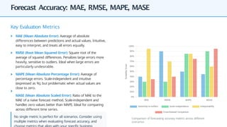


![Finance & Stock Market Forecasting
ARIMA for Stock Price Forecasting
This example demonstrates using ARIMA to forecast stock prices for
a 10- day horizon:
import pandas as pd
import numpy as np
from statsmodels.tsa.arima.model import ARIMA import
matplotlib.pyplot as plt
# Load historical stock data
df = pd.read_csv('tech_stock.csv') df['Date'] =
pd.to_datetime(df['Date']) df = df.set_index('Date')
# Fit ARIMA model (order=3,1,2)
model = ARIMA(df['Close'], order=(3,1,2)) results =
model.fit()
# Generate forecast
forecast = results.forecast(steps=10) forecast_index =
pd.date_range( start=df.index[-1] + pd.Timedelta('1
day'), periods=10, freq='B')
forecast_series = pd.Series(forecast,
index=forecast_index)
Time Series in Financial Markets
Financial markets generate vast amounts of time-ordered data that
make them ideal candidates for time series analysis. Stock prices,
exchange rates, and trading volumes all follow temporal patterns
that can be modeled and forecasted.
Financial time series often exhibit unique
characteristics like volatility clustering and leverage effects
that require specialized models.
Market Efficiency: Markets react quickly to new
information, making prediction challenging but possible in
certain timeframes
Volatility Modeling: GARCH models capture changing
variance in financial returns
Technical Analysis: Using historical price patterns to
predict future movements
Risk Management: Value-at-Risk (VaR) calculations rely on
time series forecasting
Algorithmic Trading: Automated strategies often use
time series signals](https://image.slidesharecdn.com/timeseriesanalysiscompleteguide20250816175008-250907100830-1752d98d/85/time_series_analysis_complete_guide_20250816175008-pptx-71-320.jpg)
![Economics and Macroeconomic Forecasting
Practical Example: GDP Forecasting
Using ARIMA to forecast quarterly GDP growth and inform
policy decisions:
import pandas as pd
import statsmodels.api as sm
# Load quarterly GDP data
gdp_data = pd.read_csv('quarterly_gdp.csv', parse_dates= ['date'])
gdp_data = gdp_data.set_index('date')
# Fit SARIMA model (accounts for seasonality in economic data)
model = sm.tsa.SARIMAX(gdp_data['gdp_growth'],
order=(2,1,2), # ARIMA parameters
seasonal_order=(1,1,1,4)) # Seasonal component results =
model.fit()
# Generate forecast for next 8 quarters (2 years) forecast =
results.get_forecast(steps=8) conf_int = forecast.conf_int()
Macroeconomic Time Series & Policy
Macroeconomic forecasting uses time series models to predict
future values of key economic indicators, providing critical
information for central banks, governments, and businesses to make
informed decisions.
Time series forecasts directly influence monetary policy,
fiscal planning, and regulatory frameworks that affect
entire economies.
GDP growth prediction influences government spending and
taxation policies
Inflation forecasting guides central bank interest rate
decisions
Unemployment rate projections impact labor market
policies Foreign exchange predictions affect international
trade strategies
Consumer confidence index forecasts influence retail
sector planning](https://image.slidesharecdn.com/timeseriesanalysiscompleteguide20250816175008-250907100830-1752d98d/85/time_series_analysis_complete_guide_20250816175008-pptx-72-320.jpg)
![Business Operations & Demand Forecasting
Retail Inventory Optimization
A national retailer implemented time series forecasting to
optimize inventory across 500 stores:
import pandas as pd
from statsmodels.tsa.holtwinters import
ExponentialSmoothing
# Load historical sales data
sales_data = pd.read_csv('store_sales.csv') sales_data['Date'] =
pd.to_datetime(sales_data['Date']) sales_data =
sales_data.set_index('Date')
sales_data = sales_data.asfreq('D')
# Apply Holt-Winters method with weekly seasonality model =
ExponentialSmoothing(
sales_data['Units'],
seasonal='multiplicative',
seasonal_periods=7
).fit()
# Generate 30-day forecast forecast
= model.forecast(30)
Critical for Business Success
Demand forecasting is the process of predicting future customer
demand for products or services, enabling businesses to make
informed decisions about inventory management, staffing, and
resource allocation.
Companies that effectively implement demand forecasting
can reduce costs by 10-20% while improving customer
satisfaction through optimal inventory levels.
Enables optimal inventory levels, reducing carrying costs and
stockouts Supports efficient staffing and resource planning
Improves cash flow management and financial planning
Enhances supplier relationships through consistent ordering
patterns
Supports strategic decision-making for product
development and marketing
Common forecasting methods include time series approaches
(ARIMA, exponential smoothing), machine learning models, and
causal models that incorporate external factors like promotions,](https://image.slidesharecdn.com/timeseriesanalysiscompleteguide20250816175008-250907100830-1752d98d/85/time_series_analysis_complete_guide_20250816175008-pptx-73-320.jpg)
![Healthcare and Life Sciences Applications
ECG Anomaly Detection Example
ECG monitoring generates time series data that can be analyzed to
detect abnormal heart rhythms. Below is an approach using LSTM
networks:
import pandas as pd
import numpy as np
from tensorflow.keras.models import Sequential from
tensorflow.keras.layers import LSTM, Dense
# Load ECG time series data
ecg_data = pd.read_csv('patient_ecg.csv')
# Prepare sequences for LSTM
def create_sequences(data, seq_length): X, y = [],
[]
for i in range(len(data) - seq_length):
X.append(data[i:i+seq_length])
y.append(data[i+seq_length])
return np.array(X), np.array(y)
# Train anomaly detection model
model = Sequential([
LSTM(64, input_shape=(sequence_length, 1),
Time Series in Patient Monitoring
Time series analysis plays a critical role in healthcare by enabling the
monitoring of patient vital signs, disease progression, and treatment
efficacy over time. These applications help clinicians detect anomalies
and make data-driven decisions.
Why it matters: Early detection of deteriorating conditions
through time series pattern recognition can save lives and
reduce healthcare costs.
Real-time monitoring of vital signs (heart rate, blood pressure,
glucose) Detection of arrhythmias and other cardiac
abnormalities
Prediction of patient deterioration in ICU settings
Long-term disease progression tracking (diabetes,
Parkinson's) Monitoring treatment efficacy and
medication adherence
Case Study: Early Warning Systems](https://image.slidesharecdn.com/timeseriesanalysiscompleteguide20250816175008-250907100830-1752d98d/85/time_series_analysis_complete_guide_20250816175008-pptx-74-320.jpg)
![Energy, Utilities & IoT Analytics
Balancing electricity supply
and demand through
forecasting models
Consumption pattern analysis
for billing and personalized
recommendations
Smart Meter Load Forecasting
Smart meters generate hourly or 15-minute interval electricity
consumption data. This example shows how to forecast load using
SARIMA models:
import pandas as pd
from statsmodels.tsa.statespace.sarimax import SARIMAX
# Load smart meter data
energy_data = pd.read_csv('smart_meter_readings.csv',
parse_dates=['timestamp'],
index_col='timestamp')
# Train SARIMA model (captures daily and weekly patterns) model =
SARIMAX(energy_data['kwh_consumption'], order=(1, 1, 1),
seasonal_order=(1, 1, 1, 24)) results =
model.fit()
# Generate forecasts for next 48 hours forecast
= results.forecast(steps=48)
Time Series in Smart Systems
Energy, utilities, and IoT sectors generate vast volumes of time-
stamped data from sensors, smart meters, and connected devices.
Time series analysis enables these industries to optimize operations,
reduce costs, and improve service reliability.
91% of utility companies reported improved operational
efficiency after implementing time series analytics for load
forecasting and predictive maintenance.
Granular data collection (seconds to days) enables precise
monitoring Anomaly detection identifies equipment failures
before they occur Seasonal patterns help optimize resource
allocation
Real-time analytics enable dynamic pricing and demand
response
Smart Grid Management Smart Metering](https://image.slidesharecdn.com/timeseriesanalysiscompleteguide20250816175008-250907100830-1752d98d/85/time_series_analysis_complete_guide_20250816175008-pptx-75-320.jpg)


![SMART-INDIA-HACKATHON-2025[1].ppkow it tx](https://cdn.slidesharecdn.com/ss_thumbnails/smart-india-hackathon-20251-250905190516-fd13dd80-thumbnail.jpg?width=560&fit=bounds)

