SlideShare a Scribd company logo
DATABASE MANAGEMENT SYSTEMS

    MALLA REDDY ENGG. COLLEGE HYD

     II B. Tech CSE       II Semester

           UNIT-VIII PPT SLIDES

Text Books: (1) DBMS by Raghu Ramakrishnan
            (2) DBMS by Sudarshan and Korth
INDEX
                       UNIT-8 PPT SLIDES
S.NO          Module as per                                  Lecture                PPT
              Session planner                                    No                 Slide NO
-------------------------------------------------------------------------------------------------
1.     Data on external storage &
       File organization and indexing                              L1         L1- 1 to L1- 4
2.     Index data structures                                      L2         L2- 1 to L2- 7

3.     Comparison of file organizations                            L3        L3- 1 to L3- 5

4.     Comparison of file organizations                           L4         L4- 1 to L4- 2
5.     Indexes and performance tuning                             L5         L5- 1 to L5- 4
6.     Indexes and performance tuning                             L6         L6- 1 to L6 -5
7.     Intuition for tree indexes & ISAM                          L7         L7- 1 to L7- 7

8.     B+ tree                                                    L8         L8- 1 to L8- 9
Data on External Storage
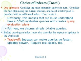
• Disks: Can retrieve random page at fixed cost
   – But reading several consecutive pages is much cheaper
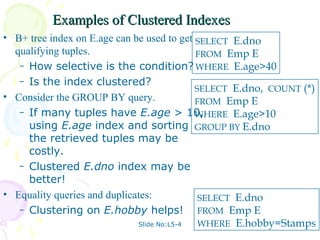
     than reading them in random order
• Tapes: Can only read pages in sequence
   – Cheaper than disks; used for archival storage
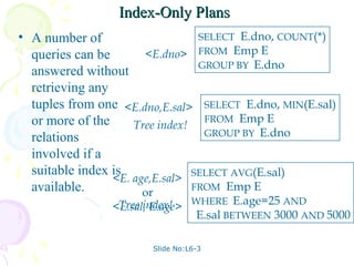
• File organization: Method of arranging a file of records on
  external storage.
   – Record id (rid) is sufficient to physically locate record
   – Indexes are data structures that allow us to find the record
     ids of records with given values in index search key fields
• Architecture: Buffer manager stages pages from external
  storage to main memory buffer pool. File and index layers
  make calls to the buffer manager.


                            Slide No:L1-1
Alternative File Organizations
Many alternatives exist, each ideal for some situations, and
  not so good in others:
   – Heap (random order) files: Suitable when typical access
     is a file scan retrieving all records.
   – Sorted Files: Best if records must be retrieved in some
     order, or only a `range’ of records is needed.
   – Indexes: Data structures to organize records via trees or
     hashing.
       • Like sorted files, they speed up searches for a subset
         of records, based on values in certain (“search key”)
         fields
       • Updates are much faster than in sorted files.


                          Slide No:L1-2
Index Classification
• Primary vs. secondary: If search key contains primary
  key, then called primary index.
   – Unique index: Search key contains a candidate key.

• Clustered vs. unclustered: If order of data records is
  the same as, or `close to’, order of data entries, then
  called clustered index.
   – Alternative 1 implies clustered; in practice,
     clustered also implies Alternative 1 (since sorted
     files are rare).
   – A file can be clustered on at most one search key.
   – Cost of retrieving data records through index varies
     greatly based on whether index is clustered or not!
                        Slide No:L1-3
Clustered vs. Unclustered Index
• Suppose that Alternative (2) is used for data entries, and that the data
  records are stored in a Heap file.
   – To build clustered index, first sort the Heap file (with some free
     space on each page for future inserts).
   – Overflow pages may be needed for inserts. (Thus, order of data
     recs is `close to’, but not identical to, the sort order.)

                            Index entries
                            direct search for
                            data entries


 CLUSTERED                                                                      UNCLUSTERED

                            Data entries                 Data entries
                                            (Index File)
                                                (Data file)


                       Data Records                              Data Records


                                      Slide No:L1-4
Indexes
• An index on a file speeds up selections on the
  search key fields for the index.
   – Any subset of the fields of a relation can be the
     search key for an index on the relation.
   – Search key is not the same as key (minimal set
     of fields that uniquely identify a record in a
     relation).
• An index contains a collection of data entries, and
  supports efficient retrieval of all data entries k*
  with a given key value k.
   – Given data entry k*, we can find record with
     key k in at most one disk I/O. (Details soon …)


                     Slide No:L2-1
B+ Tree Indexes


    Non-leaf
    Pages


    Leaf
    Pages
    (Sorted by search key)

 Leaf pages contain data entries, and are chained (prev & next)
 Non-leaf pages have index entries; only used to direct searches:

                      index entry


                 P0     K 1   P1    K 2   P 2         K m Pm


                                      Slide No:L2-2
Example B+ Tree

                               Root                                 Note how data entries
                                      17                            in leaf level are sorted

          Entries <= 17                                    Entries > 17

              5        13                                     27      30


2*   3*           5*   7* 8*    14* 16*          22* 24*           27* 29*     33* 34* 38* 39*


      • Find 28*? 29*? All > 15* and < 30*
      • Insert/delete: Find data entry in leaf, then change
        it. Need to adjust parent sometimes.
         – And change sometimes bubbles up the tree
                                           Slide No:L2-3
Hash-Based Indexes

• Good for equality selections.
• Index is a collection of buckets.
   – Bucket = primary page plus zero or more
     overflow pages.
   – Buckets contain data entries.
• Hashing function h: h(r) = bucket in which (data
  entry for) record r belongs. h looks at the search
  key fields of r.
   – No need for “index entries” in this scheme.

                      Slide No:L2-4
Alternatives for Data Entry k* in Index
• In a data entry k* we can store:
   – Data record with key value k, or
   – <k, rid of data record with search key value k>, or
   – <k, list of rids of data records with search key k>
• Choice of alternative for data entries is orthogonal to
  the indexing technique used to locate data entries with
  a given key value k.
   – Examples of indexing techniques: B+ trees, hash-
     based structures
   – Typically, index contains auxiliary information
     that directs searches to the desired data entries
                      Slide No:L2-5
Alternatives for Data Entries (Contd.)
• Alternative 1:
  – If this is used, index structure is a file
    organization for data records (instead of a Heap
    file or sorted file).
  – At most one index on a given collection of data
    records can use Alternative 1. (Otherwise, data
    records are duplicated, leading to redundant
    storage and potential inconsistency.)
  – If data records are very large, # of pages
    containing data entries is high. Implies size of
    auxiliary information in the index is also large,
    typically.

                      Slide No:L2-6
Alternatives for Data Entries (Contd.)
• Alternatives 2 and 3:
  – Data entries typically much smaller than data
    records. So, better than Alternative 1 with large
    data records, especially if search keys are small.
    (Portion of index structure used to direct search,
    which depends on size of data entries, is much
    smaller than with Alternative 1.)
  – Alternative 3 more compact than Alternative 2,
    but leads to variable sized data entries even if
    search keys are of fixed length.


                     Slide No:L2-7
Cost Model for Our Analysis
We ignore CPU costs, for simplicity:
  – B: The number of data pages
  – R: Number of records per page
  – D: (Average) time to read or write
    disk page
  – Measuring number of page I/O’s
    ignores gains of pre-fetching a
    sequence of pages; thus, even I/O cost
    is only approximated.
  – Average-case analysis; based on
    several simplistic assumptions.

                  Slide No:L3-1
Comparing File Organizations
•   Heap files (random order; insert at eof)
•   Sorted files, sorted on <age, sal>
•   Clustered B+ tree file, Alternative (1), search key
    <age, sal>
•   Heap file with unclustered B + tree index on search
    key <age, sal>
•   Heap file with unclustered hash index on search key
    <age, sal>


                        Slide No:L3-2
Operations to Compare
•   Scan: Fetch all records from disk
•   Equality search
•   Range selection
•   Insert a record
•   Delete a record


                        Slide No:L3-3
Assumptions in Our Analysis
• Heap Files:
   – Equality selection on key; exactly one match.

• Sorted Files:
   – Files compacted after deletions.

• Indexes:
   – Alt (2), (3): data entry size = 10% size of
     record
   – Hash: No overflow buckets.
      • 80% page occupancy => File size = 1.25
        data size
   – Tree: 67% occupancy (this is typical).
      • Implies file size = 1.5 data size


                    Slide No:L3-4
Assumptions (contd.)
• Scans:
   – Leaf levels of a tree-index are chained.
   – Index data-entries plus actual file
     scanned for unclustered indexes.
• Range searches:
   – We use tree indexes to restrict the set
     of data records fetched, but ignore hash
     indexes.


                   Slide No:L3-5
Cost of Operations

             (a) Scan      (b) Equality   (c ) Range   (d) Insert (e) Delete

(1) Heap     BD            0.5BD          BD           2D         Search
                                                                  +D
(2) Sorted   BD            Dlog 2B    D(log 2 B +      Search     Search
                                      # pgs with       + BD       +BD
                                      match recs)
(3)          1.5BD       Dlog F 1.5B D(log F 1.5B      Search     Search
Clustered                             + # pgs w.       +D         +D
                                      match recs)
(4) Unclust. BD(R+0.15)  D(1 +        D(log F 0.15B    Search     Search
Tree index               log F 0.15B) + # pgs w.       + 2D       + 2D
                                      match recs)
(5) Unclust. BD(R+0.125) 2D           BD               Search     Search
Hash index                                             + 2D       + 2D

                                Slide No:L4-1
Understanding the Workload
• For each query in the workload:
   – Which relations does it access?
   – Which attributes are retrieved?
   – Which attributes are involved in selection/join
     conditions? How selective are these conditions
     likely to be?
• For each update in the workload:
   – Which attributes are involved in selection/join
     conditions? How selective are these conditions
     likely to be?
   – The type of update (INSERT/DELETE/UPDATE), and
     the attributes that are affected.


                      Slide No:L4-2
Choice of Indexes


• What indexes should we create?
   – Which relations should have indexes?
     What field(s) should be the search
     key? Should we build several indexes?
• For each index, what kind of an index should it be?
   – Clustered? Hash/tree?


                     Slide No:L5-1
Choice of Indexes (Contd.)
• One approach: Consider the most important queries in turn. Consider
  the best plan using the current indexes, and see if a better plan is
  possible with an additional index. If so, create it.
   – Obviously, this implies that we must understand
     how a DBMS evaluates queries and creates query
     evaluation plans!
   – For now, we discuss simple 1-table queries.
• Before creating an index, must also consider the impact on updates in
  the workload!
   – Trade-off: Indexes can make queries go faster,
     updates slower. Require disk space, too.


                               Slide No:L5-2
Index Selection Guidelines
• Attributes in WHERE clause are candidates for index keys.
   – Exact match condition suggests hash index.
   – Range query suggests tree index.
       • Clustering is especially useful for range
         queries; can also help on equality queries if
         there are many duplicates.
• Multi-attribute search keys should be considered when a WHERE
  clause contains several conditions.
   – Order of attributes is important for range queries.
   – Such indexes can sometimes enable index-only
     strategies for important queries.
       • For index-only strategies, clustering is not
         important!


                         Slide No:L5-3
Examples of Clustered Indexes
• B+ tree index on E.age can be used to get SELECT E.dno
  qualifying tuples.                        FROM Emp E
   – How selective is the condition? WHERE E.age>40
   – Is the index clustered?
                                            SELECT E.dno, COUNT (*)
• Consider the GROUP BY query.              FROM Emp E
   – If many tuples have E.age > 10,        WHERE E.age>10
     using E.age index and sorting GROUP BY E.dno
     the retrieved tuples may be
     costly.
   – Clustered E.dno index may be
     better!
• Equality queries and duplicates:           SELECT E.dno
   – Clustering on E.hobby helps!            FROM Emp E
                              Slide No:L5-4  WHERE E.hobby=Stamps
Indexes with Composite Search Keys
• Composite Search Keys: Search on a
                                             Examples of composite key
  combination of fields.
                                             indexes using lexicographic order.
   – Equality query: Every field
      value is equal to a
      constant value. E.g. wrt
      <sal,age> index:
       • age=20 and sal =75                  11,80                                    11
                                             12,10                                    12
   – Range query: Some field                                name age sal
                                             12,20                                    12
      value is not a constant.               13,75           bob 12   10              13
      E.g.:                                 <age, sal>       cal 11   80            <age>
       • age =20; or age=20                                  joe 12   20
         and sal > 10                        10,12           sue 13   75              10
                                             20,12                                    20
• Data entries in index sorted by                           Data records
                                             75,13          sorted by name            75
  search key to support range queries.
                                             80,11                                    80
   – Lexicographic order, or
                                            <sal, age>                              <sal>
   – Spatial order.                        Data entries in index           Data entries
                                           sorted by <sal,age>             sorted by <sal>
                                  Slide No:L6-1
Composite Search Keys
• To retrieve Emp records with age=30 AND sal=4000, an
  index on <age,sal> would be better than an index on age or an
  index on sal.
   – Choice of index key orthogonal to clustering
      etc.
• If condition is: 20<age<30 AND 3000<sal<5000:
   – Clustered tree index on <age,sal> or
      <sal,age> is best.
• If condition is: age=30 AND 3000<sal<5000:
   – Clustered <age,sal> index much better than
      <sal,age> index!
• Composite indexes are larger, updated more often.
                          Slide No:L6-2
Index-Only Plans
• A number of                     SELECT E.dno, COUNT(*)
  queries can be       <E.dno> FROM Emp E
                                  GROUP BY E.dno
  answered without
  retrieving any
  tuples from one <E.dno,E.sal> SELECT E.dno, MIN(E.sal)
  or more of the                   FROM Emp E
                     Tree index!
  relations                        GROUP BY E.dno

  involved if a
  suitable index is
                 <E. age,E.sal> SELECT AVG(E.sal)
  available.           or        FROM Emp E

                <E.sal, E.age> WHERE E.age=25 AND
                 Tree index!
                                E.sal BETWEEN 3000 AND 5000

                       Slide No:L6-3
Summary
• Many alternative file organizations exist, each
  appropriate in some situation.
• If selection queries are frequent, sorting the file or
  building an index is important.
   – Hash-based indexes only good for
      equality search.
   – Sorted files and tree-based indexes best
      for range search; also good for equality
      search. (Files rarely kept sorted in
      practice; B+ tree index is better.)
• Index is a collection of data entries plus a way to
  quickly find entries with given key values.
                        Slide No:L6-4
Summary (Contd.)

• Data entries can be actual data records, <key, rid>
  pairs, or <key, rid-list> pairs.
   – Choice orthogonal to indexing
     technique used to locate data entries
     with a given key value.
• Can have several indexes on a given file of data
  records, each with a different search key.
• Indexes can be classified as clustered vs.
  unclustered, primary vs. secondary, and dense vs.
  sparse. Differences have important consequences
  for utility/performance.
                      Slide No:L6-5
Introduction
•   As for any index, 3 alternatives for data entries k*:
     – Data record with key value k
     – <k, rid of data record with search key
       value k>
     – <k, list of rids of data records with
       search key k>
•   Choice is orthogonal to the indexing technique used
    to locate data entries k*.
•   Tree-structured indexing techniques support both
    range searches and equality searches.
•   ISAM: static structure; B+ tree: dynamic, adjusts
    gracefully under inserts and deletes.
                        Slide No:L7-1
Range Searches
• ``Find all students with gpa > 3.0’’
   – If data is in sorted file, do binary
     search to find first such student, then
     scan to find others.
   – Cost of binary search can be quite
     high.
• Simple idea: Create an `index’ file.
           k1 k2                           kN            Index File


  Page 1     Page 2    Page 3                   Page N   Data File


                           Slide No:L7-2
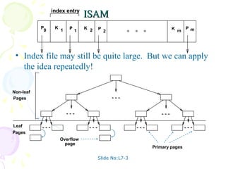
index entry
                                 ISAM
           P     K       P       K 2   P                       K m     Pm
            0        1       1             2


 • Index file may still be quite large. But we can apply
   the idea repeatedly!

Non-leaf
Pages


Leaf
Pages
                     Overflow
                       page
                                                       Primary pages

                                       Slide No:L7-3
Comments on ISAM
                                                        Data
                                                        Pages
• File creation: Leaf (data) pages allocated
     sequentially, sorted by search key; then index
     pages allocated, then space for overflow pages.      Index Pages
• Index entries: <search key value, page id>; they
  `direct’ search for data entries, which are in leaf
  pages.                                                 Overflow pages

• Search: Start at root; use key comparisons to go
  to leaf. Cost log F N ; F = # entries/index pg, N
  = # leaf pgs
          ∝
• Insert: Find leaf data entry belongs to, and put it
  there.
• Delete: Find and remove from leaf; if empty
  overflow page, de-allocate.
                               Slide No:L7-4
Example ISAM Tree
• Each node can hold 2 entries; no need for `next-leaf-
  page’ pointers. (Why?)


                    Root
                                  40


             20    33                                   51   63


 10*   15*   20*   27*     33*   37*     40*     46*   51*   55*   63*   97*


                                 Slide No:L7-5
After Inserting 23*, 48*, 41*, 42* ...


                              Root
Index                                       40

Pages


                       20    33                               51   63


Primary
Leaf
           10*   15*   20*   27*     33*   37*   40*   46*   51*   55*   63*   97*
Pages


Overflow               23*                       48*   41*

Pages
                                                 42*


                                     Slide No:L7-6
... Then Deleting 42*, 51*, 97*


                   Root
                                 40


            20    33                              51   63


10*   15*   20*   27*     33*   37*   40*   46*        55*   63*


            23*                       48*   41*


                           Slide No:L7-7
B+ Tree: Most Widely Used Index
• Insert/delete at log F N cost; keep tree height-balanced.
   (F = fanout, N = # leaf pages)
• Minimum 50% occupancy (except for root). Each
  node contains d <= m <= 2d entries. The parameter
  d is called the order of the tree.
• Supports equality and range-searches efficiently.
                                             Index Entries
                                             (Direct search)


                                             Data Entries
                                             ("Sequence set")


                          Slide No:L8-1
Example B+ Tree
• Search begins at root, and key comparisons direct it
  to a leaf (as in ISAM).
• Search for 5*, 15*, all data entries >= 24* ...


                              Root


                                     13     17     24   30


2*   3*   5*   7*   14* 16*               19* 20* 22*        24* 27* 29*   33* 34* 38* 39*


                                           Slide No:L8-2
B+ Trees in Practice
• Typical order: 100. Typical fill-factor: 67%.
   – average fanout = 133
• Typical capacities:
   – Height 4: 1334 = 312,900,700 records
   – Height 3: 1333 =          2,352,637 records
• Can often hold top levels in buffer pool:
   – Level 1 =            1 page =           8 Kbytes
   – Level 2 =        133 pages =           1 Mbyte
   – Level 3 = 17,689 pages = 133 MBytes


                       Slide No:L8-3
Inserting a Data Entry into a B+ Tree
• Find correct leaf L.
• Put data entry onto L.
   – If L has enough space, done!
   – Else, must split L (into L and a new node L2)

       • Redistribute entries evenly, copy up middle
         key.
       • Insert index entry pointing to L2 into parent
         of L.
• This can happen recursively
   – To split index node, redistribute entries evenly,
     but push up middle key. (Contrast with leaf
     splits.)
• Splits “grow” tree; root split increases height.
   – Tree growth: gets wider or one level taller at
     top.                   Slide No:L8-4
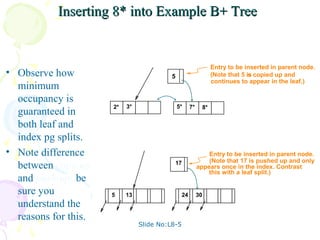
Inserting 8* into Example B+ Tree


                                                                    Entry to be inserted in parent node.
• Observe how                             5                         (Note that 5 is copied up and
                                                                                  s
                                                                    continues to appear in the leaf.)
  minimum
  occupancy is
                      2*   3*                 5*     7*        8*
  guaranteed in
  both leaf and
  index pg splits.
• Note difference                                             Entry to be inserted in parent node.
                                                              (Note that 17 is pushed up and only
  between copy-up                          17
                                                          appears once in the index. Contrast
                                                              this with a leaf split.)
  and push-up; be
  sure you            5    13                   24        30
  understand the
  reasons for this.
                                Slide No:L8-5
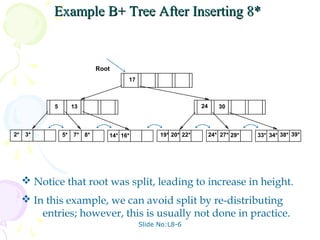
Example B+ Tree After Inserting 8*


                             Root
                                      17


            5        13                                        24      30


2*   3*         5*   7* 8*      14* 16*          19* 20* 22*        24* 27* 29*   33* 34* 38* 39*


      Notice that root was split, leading to increase in height.
      In this example, we can avoid split by re-distributing
         entries; however, this is usually not done in practice.
                                           Slide No:L8-6
Deleting a Data Entry from a B+ Tree
• Start at root, find leaf L where entry belongs.
• Remove the entry.
   – If L is at least half-full, done!
   – If L has only d-1 entries,

       • Try to re-distribute, borrowing from sibling
         (adjacent node with same parent as L).
       • If re-distribution fails, merge L and sibling.
• If merge occurred, must delete entry (pointing to L or sibling)
  from parent of L.
• Merge could propagate to root, decreasing height.


                          Slide No:L8-7
Example Tree After (Inserting 8*, Then)
                Deleting 19* and 20* ...

                             Root

                                    17


            5        13                                  27      30


2*   3*         5*   7* 8*    14* 16*          22* 24*        27* 29*   33* 34* 38* 39*


      • Deleting 19* is easy.
      • Deleting 20* is done with re-distribution. Notice
        how middle key is copied up.
                                         Slide No:L8-8
... And Then Deleting 24*


• Must merge.
                                                                    30

• Observe `toss’ of index
  entry (on right), and                        22*    27*                             38*   39*
                                                            29*          33*    34*
  `pull down’ of index
  entry (below).
                Root
                            5      13     17         30


2*   3*    5*     7*   8*       14* 16*               22* 27* 29*              33* 34* 38* 39*

                                   Slide No:L8-9

More Related Content

What's hot (20)

PPT
Linux - Introductions to Linux Operating System
Vibrant Technologies & Computers
 
PPTX
Cookies in servlets.ppt
Swetha S
 
PPT
windows 7 .ppt
salihazameer
 
PPTX
SOFTWARE PARADIGM
DrThenmozhiKarunanit
 
PPT
Hadoop Map Reduce
VNIT-ACM Student Chapter
 
PPTX
NoSQL Data Architecture Patterns
Maynooth University
 
PDF
Big Data: an introduction
Bart Vandewoestyne
 
PPT
Advanced Database Management System_Introduction Slide.ppt
BikalAdhikari4
 
PPT
Hive(ppt)
Abhinav Tyagi
 
PPT
Unit 3 chapter 1-file management
Kalai Selvi
 
PDF
Distributed Database practicals
Vrushali Lanjewar
 
PDF
Dremel Paper Review
Arinto Murdopo
 
PDF
Static Analysis Techniques For Testing Application Security - Houston Tech Fest
Denim Group
 
PDF
Files and data storage
Zaid Shabbir
 
PDF
Debugging distributed systems
Bert Jan Schrijver
 
PPT
12. Indexing and Hashing in DBMS
koolkampus
 
PPTX
Distributed Database Management System
AAKANKSHA JAIN
 
PPTX
Clustering paradigms and Partitioning Algorithms
Umang MIshra
 
DOCX
Datastructures and algorithms prepared by M.V.Brehmanada Reddy
Malikireddy Bramhananda Reddy
 
Linux - Introductions to Linux Operating System
Vibrant Technologies & Computers
 
Cookies in servlets.ppt
Swetha S
 
windows 7 .ppt
salihazameer
 
SOFTWARE PARADIGM
DrThenmozhiKarunanit
 
Hadoop Map Reduce
VNIT-ACM Student Chapter
 
NoSQL Data Architecture Patterns
Maynooth University
 
Big Data: an introduction
Bart Vandewoestyne
 
Advanced Database Management System_Introduction Slide.ppt
BikalAdhikari4
 
Hive(ppt)
Abhinav Tyagi
 
Unit 3 chapter 1-file management
Kalai Selvi
 
Distributed Database practicals
Vrushali Lanjewar
 
Dremel Paper Review
Arinto Murdopo
 
Static Analysis Techniques For Testing Application Security - Houston Tech Fest
Denim Group
 
Files and data storage
Zaid Shabbir
 
Debugging distributed systems
Bert Jan Schrijver
 
12. Indexing and Hashing in DBMS
koolkampus
 
Distributed Database Management System
AAKANKSHA JAIN
 
Clustering paradigms and Partitioning Algorithms
Umang MIshra
 
Datastructures and algorithms prepared by M.V.Brehmanada Reddy
Malikireddy Bramhananda Reddy
 

Viewers also liked (20)

PPT
Unit 07 dbms
anuragmbst
 
PPT
Unit01 dbms 2
Venkat Reddy
 
PPT
Les11
arnold 7490
 
PPT
Unit 01 dbms
anuragmbst
 
PPT
Indexing and hashing
Jeet Poria
 
PPT
b+ tree
bitistu
 
PPT
Les13
arnold 7490
 
PPT
Les01
arnold 7490
 
PPT
Les06
arnold 7490
 
PPT
Les10
arnold 7490
 
PPT
Les03
arnold 7490
 
PPT
Les09
arnold 7490
 
PPT
Les02
arnold 7490
 
PPT
Les12
arnold 7490
 
PDF
Unit 1 watertech1 merged
anuragmbst
 
PPTX
B+ Tree
cesarpa
 
PPT
Unit 03 dbms
anuragmbst
 
PPT
Unit 04 dbms
anuragmbst
 
PPT
Unit 05 dbms
anuragmbst
 
Unit 07 dbms
anuragmbst
 
Unit01 dbms 2
Venkat Reddy
 
Unit 01 dbms
anuragmbst
 
Indexing and hashing
Jeet Poria
 
b+ tree
bitistu
 
Unit 1 watertech1 merged
anuragmbst
 
B+ Tree
cesarpa
 
Unit 03 dbms
anuragmbst
 
Unit 04 dbms
anuragmbst
 
Unit 05 dbms
anuragmbst
 
Ad

Similar to Unit 08 dbms (20)

PPT
INDEXING METHODS USED IN DATABASE STORAGE
polin38
 
PPT
StorageIndexing_CS541.ppt indexes for dtata bae
syedalishahid6
 
PPT
StorageIndexing_Main memory (RAM) for currently used data. Disk for the main ...
masooda5
 
PPT
Unit08 dbms
arnold 7490
 
PPT
Mba admission in india
Edhole.com
 
PPT
Indexing and hashing
Abdul mannan Karim
 
PPT
9910559 jjjgjgjfs lke lwmerfml lew we.ppt
abduganiyevbekzod011
 
PPT
Tree-structured indexes lectures for student.ppt
abduganiyevbekzod011
 
PPTX
DBMS-Unit5-PPT.pptx important for revision
yuvivarmaa
 
PDF
Modern Database Systems - Lecture 01
Michael Mathioudakis
 
PPT
Database Management Systems index Concepts
bhaskar810658
 
PPT
Database Management Systems full lecture
thiru12741550
 
PDF
Index management in depth
Andrea Giuliano
 
PPT
File organization 1
Rupali Rana
 
PPT
Query processing and optimization
Arif A.
 
PPTX
files,indexing,hashing,linear and non linear hashing
Rohit Kumar
 
PPT
MYCH8 database management system in .ppt
ubaidullah75790
 
PPTX
Database Management System-Module-IV(part-1).pptx
AiswaryaMohan31
 
PPTX
The last mile from db to disk
Bartosz Sypytkowski
 
PPT
[Www.pkbulk.blogspot.com]file and indexing
AnusAhmad
 
INDEXING METHODS USED IN DATABASE STORAGE
polin38
 
StorageIndexing_CS541.ppt indexes for dtata bae
syedalishahid6
 
StorageIndexing_Main memory (RAM) for currently used data. Disk for the main ...
masooda5
 
Unit08 dbms
arnold 7490
 
Mba admission in india
Edhole.com
 
Indexing and hashing
Abdul mannan Karim
 
9910559 jjjgjgjfs lke lwmerfml lew we.ppt
abduganiyevbekzod011
 
Tree-structured indexes lectures for student.ppt
abduganiyevbekzod011
 
DBMS-Unit5-PPT.pptx important for revision
yuvivarmaa
 
Modern Database Systems - Lecture 01
Michael Mathioudakis
 
Database Management Systems index Concepts
bhaskar810658
 
Database Management Systems full lecture
thiru12741550
 
Index management in depth
Andrea Giuliano
 
File organization 1
Rupali Rana
 
Query processing and optimization
Arif A.
 
files,indexing,hashing,linear and non linear hashing
Rohit Kumar
 
MYCH8 database management system in .ppt
ubaidullah75790
 
Database Management System-Module-IV(part-1).pptx
AiswaryaMohan31
 
The last mile from db to disk
Bartosz Sypytkowski
 
[Www.pkbulk.blogspot.com]file and indexing
AnusAhmad
 
Ad

More from anuragmbst (14)

PDF
Unit 7-phaserule
anuragmbst
 
PDF
Unit 6-energy-resources
anuragmbst
 
PDF
Unit 3 polymers
anuragmbst
 
PDF
Unit 2-science-of-corrosion
anuragmbst
 
PDF
Unit 3 requirements engineering processes merged
anuragmbst
 
PPT
Unit 8
anuragmbst
 
PPT
Unit 7
anuragmbst
 
PPT
Unit 6
anuragmbst
 
PPT
Unit 5
anuragmbst
 
PPT
Unit4
anuragmbst
 
PPT
Unit2
anuragmbst
 
PPT
Unit1
anuragmbst
 
PPT
Unit 06 dbms
anuragmbst
 
PPT
Unit 02 dbms
anuragmbst
 
Unit 7-phaserule
anuragmbst
 
Unit 6-energy-resources
anuragmbst
 
Unit 3 polymers
anuragmbst
 
Unit 2-science-of-corrosion
anuragmbst
 
Unit 3 requirements engineering processes merged
anuragmbst
 
Unit 8
anuragmbst
 
Unit 7
anuragmbst
 
Unit 6
anuragmbst
 
Unit 5
anuragmbst
 
Unit4
anuragmbst
 
Unit2
anuragmbst
 
Unit1
anuragmbst
 
Unit 06 dbms
anuragmbst
 
Unit 02 dbms
anuragmbst
 

Recently uploaded (20)

PDF
Enhancing Environmental Monitoring with Real-Time Data Integration: Leveragin...
Safe Software
 
PDF
Supporting the NextGen 911 Digital Transformation with FME
Safe Software
 
PDF
“A Re-imagination of Embedded Vision System Design,” a Presentation from Imag...
Edge AI and Vision Alliance
 
PDF
Why aren't you using FME Flow's CPU Time?
Safe Software
 
PDF
FME as an Orchestration Tool with Principles From Data Gravity
Safe Software
 
PPTX
CapCut Pro PC Crack Latest Version Free Free
josanj305
 
PPTX
MARTSIA: A Tool for Confidential Data Exchange via Public Blockchain - Poster...
Michele Kryston
 
PPTX
MARTSIA: A Tool for Confidential Data Exchange via Public Blockchain - Pitch ...
Michele Kryston
 
PDF
TrustArc Webinar - Navigating APAC Data Privacy Laws: Compliance & Challenges
TrustArc
 
PDF
Bridging CAD, IBM TRIRIGA & GIS with FME: The Portland Public Schools Case
Safe Software
 
PDF
How to Visualize the ​Spatio-Temporal Data Using CesiumJS​
SANGHEE SHIN
 
PDF
Unlocking FME Flow’s Potential: Architecture Design for Modern Enterprises
Safe Software
 
PDF
Pipeline Industry IoT - Real Time Data Monitoring
Safe Software
 
PPTX
01_Approach Cyber- DORA Incident Management.pptx
FinTech Belgium
 
PDF
Hello I'm "AI" Your New _________________
Dr. Tathagat Varma
 
PDF
Quantum Threats Are Closer Than You Think – Act Now to Stay Secure
WSO2
 
PDF
Darley - FIRST Copenhagen Lightning Talk (2025-06-26) Epochalypse 2038 - Time...
treyka
 
PDF
Java 25 and Beyond - A Roadmap of Innovations
Ana-Maria Mihalceanu
 
PPTX
Mastering Authorization: Integrating Authentication and Authorization Data in...
Hitachi, Ltd. OSS Solution Center.
 
PDF
DoS Attack vs DDoS Attack_ The Silent Wars of the Internet.pdf
CyberPro Magazine
 
Enhancing Environmental Monitoring with Real-Time Data Integration: Leveragin...
Safe Software
 
Supporting the NextGen 911 Digital Transformation with FME
Safe Software
 
“A Re-imagination of Embedded Vision System Design,” a Presentation from Imag...
Edge AI and Vision Alliance
 
Why aren't you using FME Flow's CPU Time?
Safe Software
 
FME as an Orchestration Tool with Principles From Data Gravity
Safe Software
 
CapCut Pro PC Crack Latest Version Free Free
josanj305
 
MARTSIA: A Tool for Confidential Data Exchange via Public Blockchain - Poster...
Michele Kryston
 
MARTSIA: A Tool for Confidential Data Exchange via Public Blockchain - Pitch ...
Michele Kryston
 
TrustArc Webinar - Navigating APAC Data Privacy Laws: Compliance & Challenges
TrustArc
 
Bridging CAD, IBM TRIRIGA & GIS with FME: The Portland Public Schools Case
Safe Software
 
How to Visualize the ​Spatio-Temporal Data Using CesiumJS​
SANGHEE SHIN
 
Unlocking FME Flow’s Potential: Architecture Design for Modern Enterprises
Safe Software
 
Pipeline Industry IoT - Real Time Data Monitoring
Safe Software
 
01_Approach Cyber- DORA Incident Management.pptx
FinTech Belgium
 
Hello I'm "AI" Your New _________________
Dr. Tathagat Varma
 
Quantum Threats Are Closer Than You Think – Act Now to Stay Secure
WSO2
 
Darley - FIRST Copenhagen Lightning Talk (2025-06-26) Epochalypse 2038 - Time...
treyka
 
Java 25 and Beyond - A Roadmap of Innovations
Ana-Maria Mihalceanu
 
Mastering Authorization: Integrating Authentication and Authorization Data in...
Hitachi, Ltd. OSS Solution Center.
 
DoS Attack vs DDoS Attack_ The Silent Wars of the Internet.pdf
CyberPro Magazine
 

Unit 08 dbms

  • 1. DATABASE MANAGEMENT SYSTEMS MALLA REDDY ENGG. COLLEGE HYD II B. Tech CSE II Semester UNIT-VIII PPT SLIDES Text Books: (1) DBMS by Raghu Ramakrishnan (2) DBMS by Sudarshan and Korth
  • 2. INDEX UNIT-8 PPT SLIDES S.NO Module as per Lecture PPT Session planner No Slide NO ------------------------------------------------------------------------------------------------- 1. Data on external storage & File organization and indexing L1 L1- 1 to L1- 4 2. Index data structures L2 L2- 1 to L2- 7 3. Comparison of file organizations L3 L3- 1 to L3- 5 4. Comparison of file organizations L4 L4- 1 to L4- 2 5. Indexes and performance tuning L5 L5- 1 to L5- 4 6. Indexes and performance tuning L6 L6- 1 to L6 -5 7. Intuition for tree indexes & ISAM L7 L7- 1 to L7- 7 8. B+ tree L8 L8- 1 to L8- 9
  • 3. Data on External Storage • Disks: Can retrieve random page at fixed cost – But reading several consecutive pages is much cheaper than reading them in random order • Tapes: Can only read pages in sequence – Cheaper than disks; used for archival storage • File organization: Method of arranging a file of records on external storage. – Record id (rid) is sufficient to physically locate record – Indexes are data structures that allow us to find the record ids of records with given values in index search key fields • Architecture: Buffer manager stages pages from external storage to main memory buffer pool. File and index layers make calls to the buffer manager. Slide No:L1-1
  • 4. Alternative File Organizations Many alternatives exist, each ideal for some situations, and not so good in others: – Heap (random order) files: Suitable when typical access is a file scan retrieving all records. – Sorted Files: Best if records must be retrieved in some order, or only a `range’ of records is needed. – Indexes: Data structures to organize records via trees or hashing. • Like sorted files, they speed up searches for a subset of records, based on values in certain (“search key”) fields • Updates are much faster than in sorted files. Slide No:L1-2
  • 5. Index Classification • Primary vs. secondary: If search key contains primary key, then called primary index. – Unique index: Search key contains a candidate key. • Clustered vs. unclustered: If order of data records is the same as, or `close to’, order of data entries, then called clustered index. – Alternative 1 implies clustered; in practice, clustered also implies Alternative 1 (since sorted files are rare). – A file can be clustered on at most one search key. – Cost of retrieving data records through index varies greatly based on whether index is clustered or not! Slide No:L1-3
  • 6. Clustered vs. Unclustered Index • Suppose that Alternative (2) is used for data entries, and that the data records are stored in a Heap file. – To build clustered index, first sort the Heap file (with some free space on each page for future inserts). – Overflow pages may be needed for inserts. (Thus, order of data recs is `close to’, but not identical to, the sort order.) Index entries direct search for data entries CLUSTERED UNCLUSTERED Data entries Data entries (Index File) (Data file) Data Records Data Records Slide No:L1-4
  • 7. Indexes • An index on a file speeds up selections on the search key fields for the index. – Any subset of the fields of a relation can be the search key for an index on the relation. – Search key is not the same as key (minimal set of fields that uniquely identify a record in a relation). • An index contains a collection of data entries, and supports efficient retrieval of all data entries k* with a given key value k. – Given data entry k*, we can find record with key k in at most one disk I/O. (Details soon …) Slide No:L2-1
  • 8. B+ Tree Indexes Non-leaf Pages Leaf Pages (Sorted by search key)  Leaf pages contain data entries, and are chained (prev & next)  Non-leaf pages have index entries; only used to direct searches: index entry P0 K 1 P1 K 2 P 2 K m Pm Slide No:L2-2
  • 9. Example B+ Tree Root Note how data entries 17 in leaf level are sorted Entries <= 17 Entries > 17 5 13 27 30 2* 3* 5* 7* 8* 14* 16* 22* 24* 27* 29* 33* 34* 38* 39* • Find 28*? 29*? All > 15* and < 30* • Insert/delete: Find data entry in leaf, then change it. Need to adjust parent sometimes. – And change sometimes bubbles up the tree Slide No:L2-3
  • 10. Hash-Based Indexes • Good for equality selections. • Index is a collection of buckets. – Bucket = primary page plus zero or more overflow pages. – Buckets contain data entries. • Hashing function h: h(r) = bucket in which (data entry for) record r belongs. h looks at the search key fields of r. – No need for “index entries” in this scheme. Slide No:L2-4
  • 11. Alternatives for Data Entry k* in Index • In a data entry k* we can store: – Data record with key value k, or – <k, rid of data record with search key value k>, or – <k, list of rids of data records with search key k> • Choice of alternative for data entries is orthogonal to the indexing technique used to locate data entries with a given key value k. – Examples of indexing techniques: B+ trees, hash- based structures – Typically, index contains auxiliary information that directs searches to the desired data entries Slide No:L2-5
  • 12. Alternatives for Data Entries (Contd.) • Alternative 1: – If this is used, index structure is a file organization for data records (instead of a Heap file or sorted file). – At most one index on a given collection of data records can use Alternative 1. (Otherwise, data records are duplicated, leading to redundant storage and potential inconsistency.) – If data records are very large, # of pages containing data entries is high. Implies size of auxiliary information in the index is also large, typically. Slide No:L2-6
  • 13. Alternatives for Data Entries (Contd.) • Alternatives 2 and 3: – Data entries typically much smaller than data records. So, better than Alternative 1 with large data records, especially if search keys are small. (Portion of index structure used to direct search, which depends on size of data entries, is much smaller than with Alternative 1.) – Alternative 3 more compact than Alternative 2, but leads to variable sized data entries even if search keys are of fixed length. Slide No:L2-7
  • 14. Cost Model for Our Analysis We ignore CPU costs, for simplicity: – B: The number of data pages – R: Number of records per page – D: (Average) time to read or write disk page – Measuring number of page I/O’s ignores gains of pre-fetching a sequence of pages; thus, even I/O cost is only approximated. – Average-case analysis; based on several simplistic assumptions. Slide No:L3-1
  • 15. Comparing File Organizations • Heap files (random order; insert at eof) • Sorted files, sorted on <age, sal> • Clustered B+ tree file, Alternative (1), search key <age, sal> • Heap file with unclustered B + tree index on search key <age, sal> • Heap file with unclustered hash index on search key <age, sal> Slide No:L3-2
  • 16. Operations to Compare • Scan: Fetch all records from disk • Equality search • Range selection • Insert a record • Delete a record Slide No:L3-3
  • 17. Assumptions in Our Analysis • Heap Files: – Equality selection on key; exactly one match. • Sorted Files: – Files compacted after deletions. • Indexes: – Alt (2), (3): data entry size = 10% size of record – Hash: No overflow buckets. • 80% page occupancy => File size = 1.25 data size – Tree: 67% occupancy (this is typical). • Implies file size = 1.5 data size Slide No:L3-4
  • 18. Assumptions (contd.) • Scans: – Leaf levels of a tree-index are chained. – Index data-entries plus actual file scanned for unclustered indexes. • Range searches: – We use tree indexes to restrict the set of data records fetched, but ignore hash indexes. Slide No:L3-5
  • 19. Cost of Operations (a) Scan (b) Equality (c ) Range (d) Insert (e) Delete (1) Heap BD 0.5BD BD 2D Search +D (2) Sorted BD Dlog 2B D(log 2 B + Search Search # pgs with + BD +BD match recs) (3) 1.5BD Dlog F 1.5B D(log F 1.5B Search Search Clustered + # pgs w. +D +D match recs) (4) Unclust. BD(R+0.15) D(1 + D(log F 0.15B Search Search Tree index log F 0.15B) + # pgs w. + 2D + 2D match recs) (5) Unclust. BD(R+0.125) 2D BD Search Search Hash index + 2D + 2D Slide No:L4-1
  • 20. Understanding the Workload • For each query in the workload: – Which relations does it access? – Which attributes are retrieved? – Which attributes are involved in selection/join conditions? How selective are these conditions likely to be? • For each update in the workload: – Which attributes are involved in selection/join conditions? How selective are these conditions likely to be? – The type of update (INSERT/DELETE/UPDATE), and the attributes that are affected. Slide No:L4-2
  • 21. Choice of Indexes • What indexes should we create? – Which relations should have indexes? What field(s) should be the search key? Should we build several indexes? • For each index, what kind of an index should it be? – Clustered? Hash/tree? Slide No:L5-1
  • 22. Choice of Indexes (Contd.) • One approach: Consider the most important queries in turn. Consider the best plan using the current indexes, and see if a better plan is possible with an additional index. If so, create it. – Obviously, this implies that we must understand how a DBMS evaluates queries and creates query evaluation plans! – For now, we discuss simple 1-table queries. • Before creating an index, must also consider the impact on updates in the workload! – Trade-off: Indexes can make queries go faster, updates slower. Require disk space, too. Slide No:L5-2
  • 23. Index Selection Guidelines • Attributes in WHERE clause are candidates for index keys. – Exact match condition suggests hash index. – Range query suggests tree index. • Clustering is especially useful for range queries; can also help on equality queries if there are many duplicates. • Multi-attribute search keys should be considered when a WHERE clause contains several conditions. – Order of attributes is important for range queries. – Such indexes can sometimes enable index-only strategies for important queries. • For index-only strategies, clustering is not important! Slide No:L5-3
  • 24. Examples of Clustered Indexes • B+ tree index on E.age can be used to get SELECT E.dno qualifying tuples. FROM Emp E – How selective is the condition? WHERE E.age>40 – Is the index clustered? SELECT E.dno, COUNT (*) • Consider the GROUP BY query. FROM Emp E – If many tuples have E.age > 10, WHERE E.age>10 using E.age index and sorting GROUP BY E.dno the retrieved tuples may be costly. – Clustered E.dno index may be better! • Equality queries and duplicates: SELECT E.dno – Clustering on E.hobby helps! FROM Emp E Slide No:L5-4 WHERE E.hobby=Stamps
  • 25. Indexes with Composite Search Keys • Composite Search Keys: Search on a Examples of composite key combination of fields. indexes using lexicographic order. – Equality query: Every field value is equal to a constant value. E.g. wrt <sal,age> index: • age=20 and sal =75 11,80 11 12,10 12 – Range query: Some field name age sal 12,20 12 value is not a constant. 13,75 bob 12 10 13 E.g.: <age, sal> cal 11 80 <age> • age =20; or age=20 joe 12 20 and sal > 10 10,12 sue 13 75 10 20,12 20 • Data entries in index sorted by Data records 75,13 sorted by name 75 search key to support range queries. 80,11 80 – Lexicographic order, or <sal, age> <sal> – Spatial order. Data entries in index Data entries sorted by <sal,age> sorted by <sal> Slide No:L6-1
  • 26. Composite Search Keys • To retrieve Emp records with age=30 AND sal=4000, an index on <age,sal> would be better than an index on age or an index on sal. – Choice of index key orthogonal to clustering etc. • If condition is: 20<age<30 AND 3000<sal<5000: – Clustered tree index on <age,sal> or <sal,age> is best. • If condition is: age=30 AND 3000<sal<5000: – Clustered <age,sal> index much better than <sal,age> index! • Composite indexes are larger, updated more often. Slide No:L6-2
  • 27. Index-Only Plans • A number of SELECT E.dno, COUNT(*) queries can be <E.dno> FROM Emp E GROUP BY E.dno answered without retrieving any tuples from one <E.dno,E.sal> SELECT E.dno, MIN(E.sal) or more of the FROM Emp E Tree index! relations GROUP BY E.dno involved if a suitable index is <E. age,E.sal> SELECT AVG(E.sal) available. or FROM Emp E <E.sal, E.age> WHERE E.age=25 AND Tree index! E.sal BETWEEN 3000 AND 5000 Slide No:L6-3
  • 28. Summary • Many alternative file organizations exist, each appropriate in some situation. • If selection queries are frequent, sorting the file or building an index is important. – Hash-based indexes only good for equality search. – Sorted files and tree-based indexes best for range search; also good for equality search. (Files rarely kept sorted in practice; B+ tree index is better.) • Index is a collection of data entries plus a way to quickly find entries with given key values. Slide No:L6-4
  • 29. Summary (Contd.) • Data entries can be actual data records, <key, rid> pairs, or <key, rid-list> pairs. – Choice orthogonal to indexing technique used to locate data entries with a given key value. • Can have several indexes on a given file of data records, each with a different search key. • Indexes can be classified as clustered vs. unclustered, primary vs. secondary, and dense vs. sparse. Differences have important consequences for utility/performance. Slide No:L6-5
  • 30. Introduction • As for any index, 3 alternatives for data entries k*: – Data record with key value k – <k, rid of data record with search key value k> – <k, list of rids of data records with search key k> • Choice is orthogonal to the indexing technique used to locate data entries k*. • Tree-structured indexing techniques support both range searches and equality searches. • ISAM: static structure; B+ tree: dynamic, adjusts gracefully under inserts and deletes. Slide No:L7-1
  • 31. Range Searches • ``Find all students with gpa > 3.0’’ – If data is in sorted file, do binary search to find first such student, then scan to find others. – Cost of binary search can be quite high. • Simple idea: Create an `index’ file. k1 k2 kN Index File Page 1 Page 2 Page 3 Page N Data File Slide No:L7-2
  • 32. index entry ISAM P K P K 2 P K m Pm 0 1 1 2 • Index file may still be quite large. But we can apply the idea repeatedly! Non-leaf Pages Leaf Pages Overflow page Primary pages Slide No:L7-3
  • 33. Comments on ISAM Data Pages • File creation: Leaf (data) pages allocated sequentially, sorted by search key; then index pages allocated, then space for overflow pages. Index Pages • Index entries: <search key value, page id>; they `direct’ search for data entries, which are in leaf pages. Overflow pages • Search: Start at root; use key comparisons to go to leaf. Cost log F N ; F = # entries/index pg, N = # leaf pgs ∝ • Insert: Find leaf data entry belongs to, and put it there. • Delete: Find and remove from leaf; if empty overflow page, de-allocate. Slide No:L7-4
  • 34. Example ISAM Tree • Each node can hold 2 entries; no need for `next-leaf- page’ pointers. (Why?) Root 40 20 33 51 63 10* 15* 20* 27* 33* 37* 40* 46* 51* 55* 63* 97* Slide No:L7-5
  • 35. After Inserting 23*, 48*, 41*, 42* ... Root Index 40 Pages 20 33 51 63 Primary Leaf 10* 15* 20* 27* 33* 37* 40* 46* 51* 55* 63* 97* Pages Overflow 23* 48* 41* Pages 42* Slide No:L7-6
  • 36. ... Then Deleting 42*, 51*, 97* Root 40 20 33 51 63 10* 15* 20* 27* 33* 37* 40* 46* 55* 63* 23* 48* 41* Slide No:L7-7
  • 37. B+ Tree: Most Widely Used Index • Insert/delete at log F N cost; keep tree height-balanced. (F = fanout, N = # leaf pages) • Minimum 50% occupancy (except for root). Each node contains d <= m <= 2d entries. The parameter d is called the order of the tree. • Supports equality and range-searches efficiently. Index Entries (Direct search) Data Entries ("Sequence set") Slide No:L8-1
  • 38. Example B+ Tree • Search begins at root, and key comparisons direct it to a leaf (as in ISAM). • Search for 5*, 15*, all data entries >= 24* ... Root 13 17 24 30 2* 3* 5* 7* 14* 16* 19* 20* 22* 24* 27* 29* 33* 34* 38* 39* Slide No:L8-2
  • 39. B+ Trees in Practice • Typical order: 100. Typical fill-factor: 67%. – average fanout = 133 • Typical capacities: – Height 4: 1334 = 312,900,700 records – Height 3: 1333 = 2,352,637 records • Can often hold top levels in buffer pool: – Level 1 = 1 page = 8 Kbytes – Level 2 = 133 pages = 1 Mbyte – Level 3 = 17,689 pages = 133 MBytes Slide No:L8-3
  • 40. Inserting a Data Entry into a B+ Tree • Find correct leaf L. • Put data entry onto L. – If L has enough space, done! – Else, must split L (into L and a new node L2) • Redistribute entries evenly, copy up middle key. • Insert index entry pointing to L2 into parent of L. • This can happen recursively – To split index node, redistribute entries evenly, but push up middle key. (Contrast with leaf splits.) • Splits “grow” tree; root split increases height. – Tree growth: gets wider or one level taller at top. Slide No:L8-4
  • 41. Inserting 8* into Example B+ Tree Entry to be inserted in parent node. • Observe how 5 (Note that 5 is copied up and s continues to appear in the leaf.) minimum occupancy is 2* 3* 5* 7* 8* guaranteed in both leaf and index pg splits. • Note difference Entry to be inserted in parent node. (Note that 17 is pushed up and only between copy-up 17 appears once in the index. Contrast this with a leaf split.) and push-up; be sure you 5 13 24 30 understand the reasons for this. Slide No:L8-5
  • 42. Example B+ Tree After Inserting 8* Root 17 5 13 24 30 2* 3* 5* 7* 8* 14* 16* 19* 20* 22* 24* 27* 29* 33* 34* 38* 39*  Notice that root was split, leading to increase in height.  In this example, we can avoid split by re-distributing entries; however, this is usually not done in practice. Slide No:L8-6
  • 43. Deleting a Data Entry from a B+ Tree • Start at root, find leaf L where entry belongs. • Remove the entry. – If L is at least half-full, done! – If L has only d-1 entries, • Try to re-distribute, borrowing from sibling (adjacent node with same parent as L). • If re-distribution fails, merge L and sibling. • If merge occurred, must delete entry (pointing to L or sibling) from parent of L. • Merge could propagate to root, decreasing height. Slide No:L8-7
  • 44. Example Tree After (Inserting 8*, Then) Deleting 19* and 20* ... Root 17 5 13 27 30 2* 3* 5* 7* 8* 14* 16* 22* 24* 27* 29* 33* 34* 38* 39* • Deleting 19* is easy. • Deleting 20* is done with re-distribution. Notice how middle key is copied up. Slide No:L8-8
  • 45. ... And Then Deleting 24* • Must merge. 30 • Observe `toss’ of index entry (on right), and 22* 27* 38* 39* 29* 33* 34* `pull down’ of index entry (below). Root 5 13 17 30 2* 3* 5* 7* 8* 14* 16* 22* 27* 29* 33* 34* 38* 39* Slide No:L8-9

Editor's Notes