SlideShare a Scribd company logo
UNIT – II
Graph Algorithms
• Graph algorithms: Representations of graphs
• Graph traversal: DFS – BFS – applications
• Connectivity, strong connectivity, bi-
connectivity
• Minimum spanning tree: Kruskal’s and Prim’s
algorithm
• Shortest path: Bellman-Ford algorithm -
Dijkstra’s algorithm - Floyd-Warshall algorithm
• Network flow: Flow networks - Ford-Fulkerson
method
• Matching: Maximum bipartite matching
• A graph is a non-linear data structure made of two
components, a set of vertex V and the set of edges E.
• A graph is G= (V, E) where G is graph.
• The graph may be directed or undirected.
• Vertices are referred to as nodes and the arc between
the nodes are referred to as Edges.
• Directed graph
A directed graph G is also called digraph. Each
edge in G is identified with an order pair(U,V) of
node in G rather than an unordered pair
• Undirected graph
An undirected graph g is a graph in which each
edge e is not assigned a direction.
• V(G) = {A, B, C, D, E}
• E(G) = {(A, B), (B, C),(A, D), (B, D), (D, E), (C, E)}
• There are five vertices or nodes and six edges in
the graph (undirected graph)
Example for Graph
• A graph can be directed or undirected.
• If there is an edge from A to B, then there is a
path from A to B but not from B to A.
• The edge (A, B) is said to initiate from node A
(also known as initial node) and terminate at
node B (terminal node).
Terminology of a Directed Graph
• Out-degree of a node
• In-degree of a node
• Degree of a node
• Isolated vertex
• Source
• Sink
• Strongly connected directed graph
• Weakly connected digraph
Graph Terminology
• Adjacent nodes or neighbours
• Degree of a node - the total number of edges
containing the node
• If degree of a node is 0, such a node is known as an
isolated node.
• Regular graph - It is a graph where each vertex has
the same number of neighbours.
• Path A path P written as P = {v0, v1, v2, ..., vn}, of
length n from a node u to v is defined as a sequence of
(n+1) nodes.
• Closed path A path P is known as a closed path if the
edge has the same end-points.
• Connected graph
A graph is called connected if there is a path from
any vertex to any other vertex.
Strongly Connected Graph - If there is a path from
every vertex to every other vertex in a directed graph
then it is said to be strongly connected graph.
Otherwise, it is said to be weakly connected graph.
• Weighted Graph:
Here each edge also has
an associated real
number with it, known
as the edge weight.
• Complete Graph:
If there is an edges from
each vertices to all other
vertices in graph is
called as completed
graph.
• Path
A path is a sequence of distinct vertices, each
adjacent to the next. The length of such a path is
number of edges on that path.
• Sub Graph
A subgraph of G is a graph G’ such that V(G’)
is a subset of V(G) and E(G’) is a subset of E(G)
• Cycle
A path of non-zero length
from and to the same
vertex with no repeated
edges.
• Acyclic Graph
A directed graph which has
no cycles is referred to as
acyclic graph. It is
abbreviated as DAG
[Directed Acyclic Graph]
6
4 5
1
2
3
• Degree
The degree of a vertex is the number of edges
incident to that vertex
For directed graph,
– the in-degree of a vertex v is the number of edges
that have v as the head
– the out-degree of a vertex v is the number of edges
that have v as the tail
3
0
1 2
3
3
3
3
0
1 2
3 4 5 6
2
3 3
1 1 1 1
Graph Representations
• Adjacency Matrices (Sequential Representation)
• Adjacency Lists (Linked Representation)
• Adjacency Multilists
Adjacency Matrix:
• Graph can be represented by Adjacency
Matrix and Adjacency list. The adjacency
Matrix A for a graph G = (V, E) with n vertices
is an n x n matrix, such that
• Aij = 1, if there is an edge Vi to Vj
• Aij = 0, if there is no edge.
UNIT II - Graph Algorithms techniques.pptx
Adjacency List
• An adjacency list represents a graph as an
array of linked list.
• The index of the array represents a vertex and
each element in its linked list represents the
other vertices that form an edge with the
vertex.
UNIT II - Graph Algorithms techniques.pptx
Examples for Adjacency Matrix
0
1
1
1
1
0
1
1
1
1
0
1
1
1
1
0












0
1
0
1
0
0
0
1
0










0
1
1
0
0
0
0
0
1
0
0
1
0
0
0
0
1
0
0
1
0
0
0
0
0
1
1
0
0
0
0
0
0
0
0
0
0
1
0
0
0
0
0
0
1
0
1
0
0
0
0
0
0
1
0
1
0
0
0
0
0
0
1
0


























G1
G2
G4
0
1 2
3
0
1
2
1
0
2
3
4
5
6
7
symmetric
undirected: n2
/2
directed: n2
0
1
2
3
0
1
2
0
1
2
3
4
5
6
7
1 2 3
0 2 3
0 1 3
0 1 2
G1
1
0 2
G3
1 2
0 3
0 3
1 2
5
4 6
5 7
6
G4
0
1 2
3
0
1
2
1
0
2
3
4
5
6
7
An undirected graph with n vertices and e edges ==> n head nodes and 2e list nodes
Adjacency Multi-lists
• Adjacency Multi-lists are an edge, rather than
vertex based, graph representation.
• In the Multilist representation of graph structures;
there are two parts, a directory of Node information
and a set of linked list of edge information.
• There is one entry in the node directory for each
node of the graph.
• The directory entry for node i points to a linked
adjacency list for node i. each record of the linked
list area appears on two adjacency lists: one for the
node at each end of the represented edge.
UNIT II - Graph Algorithms techniques.pptx
Graph Traversals
There are two standard methods of graph traversal.
• Breadth First Traversal (or) Breadth-first search
- Breadth-first search (BFS) is a graph search
algorithm that begins at the root node and explores
all the neighbouring nodes.
- Then for each of those nearest nodes explores their
unexplored neighbour nodes, and so on, until it
finds the goal.
Breadth-first search Algorithm
BREADTH-FIRST SEARCH
• BFS: 0 1 3 8 7 2 4 5 6
• Depth First Traversal (or) Depth-first search
- The depth-first search (DFS) algorithm progresses by
expanding the starting node of a graph and then going
deeper and deeper until the goal node is found, or
until a node that has no children is encountered.
- When a dead-end is reached, the algorithm
backtracks, returning to the most recent node that has
not been completely explored.
Depth-first search Algorithm
DEPTH-FIRST SEARCH
• DFS: 0 1 7 2 3 4 8 5 6
Prim’s Algorithm
• Given n points, connect them in the cheapest possible
way so that there will be a path between every pair of
points.
• Applications:
– To the design of all kinds of networks — including
communication, computer, transportation, and
electrical — by providing the cheapest way to
achieve connectivity.
• We can represent the points given by vertices of a
graph, possible connections by the graph’s edges, and
the connection costs by the edge weights. Then we
have to find the minimum spanning tree.
• Minimum Spanning Tree - Definition
– A spanning tree of an undirected connected graph
is its connected acyclic subgraph that contains all
the vertices of the graph.
– If such a graph has weights assigned to its edges, a
minimum spanning tree is its spanning tree of the
smallest weight, where the weight of a tree is
defined as the sum of the weights on all its edges.
• Prim’s algorithm constructs a minimum spanning tree
through a sequence of expanding subtrees.
• The initial subtree in such a sequence consists of a
single vertex selected arbitrarily from the set V of the
graph’s vertices.
• On each iteration, the algorithm expands the current
tree in the greedy manner by simply attaching to it the
nearest vertex not in that tree.
• The algorithm stops after all the graph’s vertices have
been included in the tree being constructed.
• Since the algorithm expands a tree by exactly one
vertex on each of its iterations, the total number of
such iterations is n-1, where n is the number of
vertices.
Apply Prim’s algorithm to the following graph
Prim’s Algorithm
ALGORITHM Prim(G)
//Prim’s algorithm for constructing a minimum spanning tree
//Input: A weighted connected graph G = (V, E)
//Output: ET, the set of edges composing a minimum
//spanning tree of G
VT ←{v0}
ET ←∅
for i ←1 to |V| − 1 do
find a minimum-weight edge e∗
= (v∗
, u∗
) among all
the edges (v, u) such that v is in VT and u is in V − VT
VT← VT {u
∪ ∗
}
ET ← ET {e
∪ ∗
}
Kruskal’s Algorithm
• Kruskal’s algorithm looks at a minimum spanning
tree of a weighted connected graph G = <V, E >as an
acyclic subgraph with |V| − 1 edges for which the sum
of the edge weights is the smallest.
• This algorithm constructs a minimum spanning tree
as an expanding sequence of subgraphs that are
always acyclic
• The algorithm begins by sorting the graph’s edges in
non-decreasing order of their weights.
• Starting with the empty subgraph, it scans this sorted
list, adding the next edge on the list to the current
subgraph which does not create a cycle.
Kruskal’s Algorithm
ALGORITHM Kruskal(G)
//Kruskal’s algorithm for constructing a minimum spanning tree
//Input: A weighted connected graph G = (V, E)
//Output: ET , the set of edges composing a minimum spanning
//tree of G sort E in non-decreasing order of the edge weights
//w(ei1
) ≤ . . . ≤ w(ei|E|
)
ET ← ;
∅
ecounter ←0 //initialize the set of tree edges and its size
k←0 //initialize the number of processed edges
while ecounter < |V| − 1 do
k←k + 1
if ET {
∪ eik
} is acyclic
ET ←ET {
∪ eik
}
ecounter ←ecounter + 1
Apply Kruskal’s algorithm to find a minimum
spanning tree of the following graph.
Shortest Path Problem
 Weighted path length (cost): The sum of the
weights of all links on the path.
 The single-source shortest path problem: Given a
weighted graph G and a source vertex s, find the
shortest (minimum cost) path from s to every
other vertex in G.
Dijkstra's Algorithm
• Single-source shortest-paths problem
• For a given vertex called the source in a weighted
connected graph, find shortest paths to all its
other vertices.
• This algorithm is applicable to graphs with
nonnegative weights only.
• Dijkstra's algorithm finds the shortest paths to a
graph's vertices in order of their distance from a
given source
UNIT II - Graph Algorithms techniques.pptx
Comparison
 Negative link weight: The Bellman-Ford
algorithm works; Dijkstra’s algorithm doesn’t.
 Distributed implementation: The Bellman-Ford
algorithm can be easily implemented in a
distributed way. Dijkstra’s algorithm cannot.
 Time complexity: The Bellman-Ford algorithm
is higher than Dijkstra’s algorithm.
The Bellman-Ford Algorithm
,nil
,nil
,nil
0
6
7
9
5
-3
8
7
-4
2
,nil
s
y z
x
t
-2
The Bellman-Ford Algorithm
,nil
,nil
,nil
0
6
7
9
5
-3
8
7
-4
2
,nil
s
y z
x
t
-2
6,s
7,s
,nil
0
6
7
9
5
-3
8
7
-4
2
,nil
s
y z
x
t
-2
Initialization After pass 1
6,s
7,s
4,y
0
6
7
9
5
-3
8
7
-4
2
2,t
s
y z
x
t
-2
After pass 2
2,x
7,s
4,y
0
6
7
9
5
-3
8
7
-4
2
2,t
s
y z
x
t
-2
After pass 3
The order of edges examined in each pass:
(t, x), (t, z), (x, t), (y, x), (y, t), (y, z), (z, x), (z, s), (s, t), (s, y)
The Bellman-Ford Algorithm
After pass 4
2,x
7,s
4,y
0
6
7
9
5
-3
8
7
-4
2
-2,t
s
y z
x
t
-2
The order of edges examined in each pass:
(t, x), (t, z), (x, t), (y, x), (y, t), (y, z), (z, x), (z, s), (s, t), (s, y)
The Bellman-Ford Algorithm
Bellman-Ford(G, w, s)
Initialize-Single-Source(G, s)
for i := 1 to |V| - 1 do
for each edge (u, v)  E do
B-F(u, v, w)
for each vertex v  u.adj do
if d[v] > d[u] + w(u, v)
then return False
return True
B-F(u, v, w)
if d[v] > d[u] + w(u, v)
then d[v] := d[u] + w(u, v)
parent[v] := u
Time Complexity
Bellman-Ford(G, w, s)
1. Initialize-Single-Source(G, s)
2. for i := 1 to |V| - 1 do
3. for each edge (u, v)  E do
4. B-F(u, v, w)
5. for each vertex v  u.adj do
6. if d[v] > d[u] + w(u, v)
7. then return False // there is a negative
cycle
8. return True
O(|V|)
O(|V||E|)
O(|E|)
Time complexity: O(|V||E|)
Warshall’s Algorithm
• It is named after Stephen Warshall.
• It is used to constructs transitive closure of a
directed graph.
• The transitive closure of a directed graph with n
vertices can be defined as the n×n boolean matrix
T = {tij }, in which the element in the ith
row and the
jth
column is 1 if there exists a nontrivial path from
the ith
vertex to the jth
vertex; otherwise, tij is 0.
• Warshall’s algorithm constructs the transitive closure
through a series of n × n boolean matrices:
R(0), . . . , R(k−1), R(k), . . . R(n)
• The central point of the algorithm is to compute all
the elements of each matrix R(k)
from its immediate
predecessor R(k−1)
in series.
• Let rij
(k)
, the element in the ith
row and jth
column of
matrix R(k)
, be equal to 1. This means that there exists
a path from the ith
vertex vi to the jth
vertex vj with
each intermediate vertex numbered not higher than k.
Pseudocode
ALGORITHM Warshall(A[1..n, 1..n])
//Implements Warshall’s algorithm for computing the
//transitive closure
//Input: The adjacency matrix A of a digraph with n vertices
//Output: The transitive closure of the digraph
R(0)
←A
for k←1 to n do
for i ←1 to n do
for j ←1 to n do
R(k)
[i, j ] ← R(k−1)
[i, j ] or
(R(k−1)
[i, k] and R(k−1)
[k, j])
return R(n)
• Time Efficiency : Ө (n3
)
• Space Efficiency: Matrices can be written over
their predecessors
Exercise
• Apply Warshall’s algorithm to find the transitive
closure of the digraph defined by the following
adjacency matrix:
Floyd’sAlgorithm
• It also known as all-pairs shortest path
• This algorithm is used to find the lengths of the
shortest paths from each vertex to all other vertices in a
weighted (directed/undirected) graph.
• The lengths of shortest paths in an n×n matrix D is
called the distance matrix. The element dij in the ith
row and the jth
column of this matrix indicates the
length of the shortest path from the ith
vertex to the jth
vertex
Pseudo Code
ALGORITHM Floyd(W[1..n, 1..n])
//Implements Floyd’s algorithm for the all-pairs
shortest-//paths problem
//Input: The weight matrix W of a graph with no
negative-//length cycle
//Output: The distance matrix of the shortest paths’
//lengths
D ←W //is not necessary if W can be overwritten
for k←1 to n do
for i ←1 to n do
for j ←1 to n do
D[i, j ]←min{D[i, j ], D[i, k]+ D[k, j]}
return D
Exercise
Solve the all-pairs shortest-path problem for the digraph
with the following weight matrix:
Maximum-Flow Problem
• The problem of maximizing the flow of a
material through a transportation network
• The transportation network can be represented
by a connected weighted digraph with n
vertices numbered from 1 to n and a set of
edges E, with some properties.
Properties are,
• It contains exactly one vertex with no entering
edges, this vertex is called the source
• It contains exactly one vertex with no leaving
edges, this vertex is called the sink
• The weight uij of each directed edge (i, j) is a
positive integer, called the edge capacity.
A digraph satisfying these properties is called a
flow network or network
Flow-conservation requirement
• The source and the sink are the only source and
destination of the material respectively. All the other
vertices serve only as points where a flow can be
redirected without consuming material flow through
it.
• In other words, the total amount of the material
entering an intermediate vertex must be equal to the
total amount of the material leaving the vertex. This
condition is called the flow-conservation
requirement.
• Flow Conservation:
• The quantity of the total outflow from the
source or equivalently, the total inflow into the
sink is called the value of the flow.
Ford-Fulkerson Method
• Given a graph which represent a flow network
where every edge has a capacity. Also given
two vertices source ‘s’ and sink ‘t’ in a graph.
• Find the maximum possible flow from s to t
with some constraints,
– Flow on an edge does not exceed the given
capacity of the edge.
– In-flow must be equal to out-flow for every vertex
except source and sink.
• Residual Network/Graph:
It is a graph which indicates
additional possible flow. If there is such path
from source to sink then there is possibility to
add the flow.
• Residual Capacity
It is the original capacity which
represents capacity of edge minus flow.
• Minimal Cut
It is also known as bottle neck capacity, which
decides maximum possible flow from source
to sink through an augmented path.
• Augmenting Path
Augmenting path can classified as two types,
Non-full forward edges
Non-empty backward edges
Algorithm
• Initially Start with the flow value as 0.
• While there is an augmenting path from source
to sink, add that path flow value to flow.
• Finally return the flow
Examples
• https://cp-algorithms.com/graph/edmonds_karp.html#toc-tgt-1
UNIT II - Graph Algorithms techniques.pptx
MAXIMUM MATCHING IN BIPARTITE
GRAPHS
• Bipartite graph: a graph whose vertices can be
partitioned into two disjoint sets V and U, not
necessarily of the same size, so that every edge
connects a vertex in V to a vertex in U.
• A graph is bipartite if and only if it does not
have a cycle of an odd length.
• A bipartite graph is 2-colorable: the vertices
can be coloured in two colours so that every
edge has its vertices coloured differently.
Matching in a Graph
• A matching in a graph is a subset of its edges
with the property that no two edges share a
vertex
• A maximum (or maximum cardinality)
matching is a matching with the largest
number of edges
Theorem: A matching M is maximum if and
only if there exists no augmenting path with
respect to M.
• Start with some initial matching. e.g., the
empty set
• Find an augmenting path and augment the
current matching along that path. e.g., using
breadth-first search like method
• When no augmenting path can be found,
terminate and return the last matching, which
is maximum
UNIT II - Graph Algorithms techniques.pptx

More Related Content

Similar to UNIT II - Graph Algorithms techniques.pptx (20)

PPTX
Graph Algorithms
Ashwin Shiv
 
PPTX
ppt 1.pptx
ShasidharaniD
 
PPTX
Unit ix graph
Tribhuvan University
 
PPTX
Unit 9 graph
Dabbal Singh Mahara
 
PDF
Graphhhhhhhhhhhhhhhhhhhhhhhhhhhhhhhh.pdf
timoemin50
 
PPTX
Data Structure of computer science and technology
bhaskarsai499
 
PPSX
Unit-6 Graph.ppsx ppt
DhruvilSTATUS
 
PPT
GraphAlgorithms.pptsfjaaaaaaaaaaaaaaaaaaa
robozenbd
 
PDF
LEC 12-DSALGO-GRAPHS(final12).pdf
MuhammadUmerIhtisham
 
PPT
1535 graph algorithms
Dr Fereidoun Dejahang
 
PPT
Chap10 slides
BaliThorat1
 
PPTX
NON-LINEAR DATA STRUCTURE-Graphs.pptx
Rajitha Reddy Alugati
 
PPT
Shortest path (Dijkistra's Algorithm) & Spanning Tree (Prim's Algorithm)
Mohanlal Sukhadia University (MLSU)
 
PPT
Unit VI - Graphs.ppt
HODElex
 
PPT
Data Structures-Non Linear DataStructures-Graphs
sailaja156145
 
PPTX
Graph Data Structure
Afaq Mansoor Khan
 
PPTX
Graphs
KomalPaliwal3
 
PPTX
10.graph
jashobhan pradhan
 
PPTX
Unit II_Graph.pptxkgjrekjgiojtoiejhgnltegjte
pournima055
 
Graph Algorithms
Ashwin Shiv
 
ppt 1.pptx
ShasidharaniD
 
Unit ix graph
Tribhuvan University
 
Unit 9 graph
Dabbal Singh Mahara
 
Graphhhhhhhhhhhhhhhhhhhhhhhhhhhhhhhh.pdf
timoemin50
 
Data Structure of computer science and technology
bhaskarsai499
 
Unit-6 Graph.ppsx ppt
DhruvilSTATUS
 
GraphAlgorithms.pptsfjaaaaaaaaaaaaaaaaaaa
robozenbd
 
LEC 12-DSALGO-GRAPHS(final12).pdf
MuhammadUmerIhtisham
 
1535 graph algorithms
Dr Fereidoun Dejahang
 
Chap10 slides
BaliThorat1
 
NON-LINEAR DATA STRUCTURE-Graphs.pptx
Rajitha Reddy Alugati
 
Shortest path (Dijkistra's Algorithm) & Spanning Tree (Prim's Algorithm)
Mohanlal Sukhadia University (MLSU)
 
Unit VI - Graphs.ppt
HODElex
 
Data Structures-Non Linear DataStructures-Graphs
sailaja156145
 
Graph Data Structure
Afaq Mansoor Khan
 
Unit II_Graph.pptxkgjrekjgiojtoiejhgnltegjte
pournima055
 

Recently uploaded (20)

PPTX
Electron Beam Machining for Production Process
Rajshahi University of Engineering & Technology(RUET), Bangladesh
 
PPTX
Cyclic_Redundancy_Check_Presentation.pptx
alhjranyblalhmwdbdal
 
PPTX
File Strucutres and Access in Data Structures
mwaslam2303
 
PPTX
Mining Presentation Underground - Copy.pptx
patallenmoore
 
PDF
Lecture Information Theory and CodingPart-1.pdf
msc9219
 
PPTX
Coding about python and MySQL connectivity
inderjitsingh1985as
 
PPTX
site survey architecture student B.arch.
sri02032006
 
PDF
OT-cybersecurity-solutions-from-TXOne-Deployment-Model-Overview-202306.pdf
jankokersnik70
 
PDF
Number Theory practice session 25.05.2025.pdf
DrStephenStrange4
 
PDF
IoT - Unit 2 (Internet of Things-Concepts) - PPT.pdf
dipakraut82
 
PDF
Passive building design opening approach
Dr-Fatima Um Mgdad
 
PPTX
Pharmaceuticals and fine chemicals.pptxx
jaypa242004
 
PDF
A presentation on the Urban Heat Island Effect
studyfor7hrs
 
PPTX
原版一样(Acadia毕业证书)加拿大阿卡迪亚大学毕业证办理方法
Taqyea
 
PPTX
Heart Bleed Bug - A case study (Course: Cryptography and Network Security)
Adri Jovin
 
PPT
04 Origin of Evinnnnnnnnnnnnnnnnnnnnnnnnnnl-notes.ppt
LuckySangalala1
 
PDF
13th International Conference of Networks and Communications (NC 2025)
JohannesPaulides
 
PPTX
Structural Functiona theory this important for the theorist
cagumaydanny26
 
PDF
Detailed manufacturing Engineering and technology notes
VIKKYsing
 
PPT
Oxygen Co2 Transport in the Lungs(Exchange og gases)
SUNDERLINSHIBUD
 
Electron Beam Machining for Production Process
Rajshahi University of Engineering & Technology(RUET), Bangladesh
 
Cyclic_Redundancy_Check_Presentation.pptx
alhjranyblalhmwdbdal
 
File Strucutres and Access in Data Structures
mwaslam2303
 
Mining Presentation Underground - Copy.pptx
patallenmoore
 
Lecture Information Theory and CodingPart-1.pdf
msc9219
 
Coding about python and MySQL connectivity
inderjitsingh1985as
 
site survey architecture student B.arch.
sri02032006
 
OT-cybersecurity-solutions-from-TXOne-Deployment-Model-Overview-202306.pdf
jankokersnik70
 
Number Theory practice session 25.05.2025.pdf
DrStephenStrange4
 
IoT - Unit 2 (Internet of Things-Concepts) - PPT.pdf
dipakraut82
 
Passive building design opening approach
Dr-Fatima Um Mgdad
 
Pharmaceuticals and fine chemicals.pptxx
jaypa242004
 
A presentation on the Urban Heat Island Effect
studyfor7hrs
 
原版一样(Acadia毕业证书)加拿大阿卡迪亚大学毕业证办理方法
Taqyea
 
Heart Bleed Bug - A case study (Course: Cryptography and Network Security)
Adri Jovin
 
04 Origin of Evinnnnnnnnnnnnnnnnnnnnnnnnnnl-notes.ppt
LuckySangalala1
 
13th International Conference of Networks and Communications (NC 2025)
JohannesPaulides
 
Structural Functiona theory this important for the theorist
cagumaydanny26
 
Detailed manufacturing Engineering and technology notes
VIKKYsing
 
Oxygen Co2 Transport in the Lungs(Exchange og gases)
SUNDERLINSHIBUD
 
Ad

UNIT II - Graph Algorithms techniques.pptx

  • 1. UNIT – II Graph Algorithms
  • 2. • Graph algorithms: Representations of graphs • Graph traversal: DFS – BFS – applications • Connectivity, strong connectivity, bi- connectivity • Minimum spanning tree: Kruskal’s and Prim’s algorithm • Shortest path: Bellman-Ford algorithm - Dijkstra’s algorithm - Floyd-Warshall algorithm • Network flow: Flow networks - Ford-Fulkerson method • Matching: Maximum bipartite matching
  • 3. • A graph is a non-linear data structure made of two components, a set of vertex V and the set of edges E. • A graph is G= (V, E) where G is graph. • The graph may be directed or undirected. • Vertices are referred to as nodes and the arc between the nodes are referred to as Edges.
  • 4. • Directed graph A directed graph G is also called digraph. Each edge in G is identified with an order pair(U,V) of node in G rather than an unordered pair • Undirected graph An undirected graph g is a graph in which each edge e is not assigned a direction.
  • 5. • V(G) = {A, B, C, D, E} • E(G) = {(A, B), (B, C),(A, D), (B, D), (D, E), (C, E)} • There are five vertices or nodes and six edges in the graph (undirected graph) Example for Graph
  • 6. • A graph can be directed or undirected. • If there is an edge from A to B, then there is a path from A to B but not from B to A. • The edge (A, B) is said to initiate from node A (also known as initial node) and terminate at node B (terminal node).
  • 7. Terminology of a Directed Graph • Out-degree of a node • In-degree of a node • Degree of a node • Isolated vertex • Source • Sink • Strongly connected directed graph • Weakly connected digraph
  • 8. Graph Terminology • Adjacent nodes or neighbours • Degree of a node - the total number of edges containing the node • If degree of a node is 0, such a node is known as an isolated node. • Regular graph - It is a graph where each vertex has the same number of neighbours. • Path A path P written as P = {v0, v1, v2, ..., vn}, of length n from a node u to v is defined as a sequence of (n+1) nodes. • Closed path A path P is known as a closed path if the edge has the same end-points.
  • 9. • Connected graph A graph is called connected if there is a path from any vertex to any other vertex. Strongly Connected Graph - If there is a path from every vertex to every other vertex in a directed graph then it is said to be strongly connected graph. Otherwise, it is said to be weakly connected graph.
  • 10. • Weighted Graph: Here each edge also has an associated real number with it, known as the edge weight. • Complete Graph: If there is an edges from each vertices to all other vertices in graph is called as completed graph.
  • 11. • Path A path is a sequence of distinct vertices, each adjacent to the next. The length of such a path is number of edges on that path. • Sub Graph A subgraph of G is a graph G’ such that V(G’) is a subset of V(G) and E(G’) is a subset of E(G)
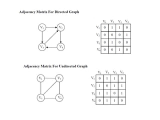
  • 12. • Cycle A path of non-zero length from and to the same vertex with no repeated edges. • Acyclic Graph A directed graph which has no cycles is referred to as acyclic graph. It is abbreviated as DAG [Directed Acyclic Graph] 6 4 5 1 2 3
  • 13. • Degree The degree of a vertex is the number of edges incident to that vertex For directed graph, – the in-degree of a vertex v is the number of edges that have v as the head – the out-degree of a vertex v is the number of edges that have v as the tail 3 0 1 2 3 3 3 3 0 1 2 3 4 5 6 2 3 3 1 1 1 1
  • 14. Graph Representations • Adjacency Matrices (Sequential Representation) • Adjacency Lists (Linked Representation) • Adjacency Multilists
  • 15. Adjacency Matrix: • Graph can be represented by Adjacency Matrix and Adjacency list. The adjacency Matrix A for a graph G = (V, E) with n vertices is an n x n matrix, such that • Aij = 1, if there is an edge Vi to Vj • Aij = 0, if there is no edge.
  • 17. Adjacency List • An adjacency list represents a graph as an array of linked list. • The index of the array represents a vertex and each element in its linked list represents the other vertices that form an edge with the vertex.
  • 19. Examples for Adjacency Matrix 0 1 1 1 1 0 1 1 1 1 0 1 1 1 1 0             0 1 0 1 0 0 0 1 0           0 1 1 0 0 0 0 0 1 0 0 1 0 0 0 0 1 0 0 1 0 0 0 0 0 1 1 0 0 0 0 0 0 0 0 0 0 1 0 0 0 0 0 0 1 0 1 0 0 0 0 0 0 1 0 1 0 0 0 0 0 0 1 0                           G1 G2 G4 0 1 2 3 0 1 2 1 0 2 3 4 5 6 7 symmetric undirected: n2 /2 directed: n2
  • 20. 0 1 2 3 0 1 2 0 1 2 3 4 5 6 7 1 2 3 0 2 3 0 1 3 0 1 2 G1 1 0 2 G3 1 2 0 3 0 3 1 2 5 4 6 5 7 6 G4 0 1 2 3 0 1 2 1 0 2 3 4 5 6 7 An undirected graph with n vertices and e edges ==> n head nodes and 2e list nodes
  • 21. Adjacency Multi-lists • Adjacency Multi-lists are an edge, rather than vertex based, graph representation. • In the Multilist representation of graph structures; there are two parts, a directory of Node information and a set of linked list of edge information. • There is one entry in the node directory for each node of the graph. • The directory entry for node i points to a linked adjacency list for node i. each record of the linked list area appears on two adjacency lists: one for the node at each end of the represented edge.
  • 24. There are two standard methods of graph traversal. • Breadth First Traversal (or) Breadth-first search - Breadth-first search (BFS) is a graph search algorithm that begins at the root node and explores all the neighbouring nodes. - Then for each of those nearest nodes explores their unexplored neighbour nodes, and so on, until it finds the goal.
  • 26. BREADTH-FIRST SEARCH • BFS: 0 1 3 8 7 2 4 5 6
  • 27. • Depth First Traversal (or) Depth-first search - The depth-first search (DFS) algorithm progresses by expanding the starting node of a graph and then going deeper and deeper until the goal node is found, or until a node that has no children is encountered. - When a dead-end is reached, the algorithm backtracks, returning to the most recent node that has not been completely explored.
  • 29. DEPTH-FIRST SEARCH • DFS: 0 1 7 2 3 4 8 5 6
  • 30. Prim’s Algorithm • Given n points, connect them in the cheapest possible way so that there will be a path between every pair of points. • Applications: – To the design of all kinds of networks — including communication, computer, transportation, and electrical — by providing the cheapest way to achieve connectivity. • We can represent the points given by vertices of a graph, possible connections by the graph’s edges, and the connection costs by the edge weights. Then we have to find the minimum spanning tree.
  • 31. • Minimum Spanning Tree - Definition – A spanning tree of an undirected connected graph is its connected acyclic subgraph that contains all the vertices of the graph. – If such a graph has weights assigned to its edges, a minimum spanning tree is its spanning tree of the smallest weight, where the weight of a tree is defined as the sum of the weights on all its edges. • Prim’s algorithm constructs a minimum spanning tree through a sequence of expanding subtrees. • The initial subtree in such a sequence consists of a single vertex selected arbitrarily from the set V of the graph’s vertices.
  • 32. • On each iteration, the algorithm expands the current tree in the greedy manner by simply attaching to it the nearest vertex not in that tree. • The algorithm stops after all the graph’s vertices have been included in the tree being constructed. • Since the algorithm expands a tree by exactly one vertex on each of its iterations, the total number of such iterations is n-1, where n is the number of vertices.
  • 33. Apply Prim’s algorithm to the following graph
  • 34. Prim’s Algorithm ALGORITHM Prim(G) //Prim’s algorithm for constructing a minimum spanning tree //Input: A weighted connected graph G = (V, E) //Output: ET, the set of edges composing a minimum //spanning tree of G VT ←{v0} ET ←∅ for i ←1 to |V| − 1 do find a minimum-weight edge e∗ = (v∗ , u∗ ) among all the edges (v, u) such that v is in VT and u is in V − VT VT← VT {u ∪ ∗ } ET ← ET {e ∪ ∗ }
  • 35. Kruskal’s Algorithm • Kruskal’s algorithm looks at a minimum spanning tree of a weighted connected graph G = <V, E >as an acyclic subgraph with |V| − 1 edges for which the sum of the edge weights is the smallest. • This algorithm constructs a minimum spanning tree as an expanding sequence of subgraphs that are always acyclic • The algorithm begins by sorting the graph’s edges in non-decreasing order of their weights. • Starting with the empty subgraph, it scans this sorted list, adding the next edge on the list to the current subgraph which does not create a cycle.
  • 36. Kruskal’s Algorithm ALGORITHM Kruskal(G) //Kruskal’s algorithm for constructing a minimum spanning tree //Input: A weighted connected graph G = (V, E) //Output: ET , the set of edges composing a minimum spanning //tree of G sort E in non-decreasing order of the edge weights //w(ei1 ) ≤ . . . ≤ w(ei|E| ) ET ← ; ∅ ecounter ←0 //initialize the set of tree edges and its size k←0 //initialize the number of processed edges while ecounter < |V| − 1 do k←k + 1 if ET { ∪ eik } is acyclic ET ←ET { ∪ eik } ecounter ←ecounter + 1
  • 37. Apply Kruskal’s algorithm to find a minimum spanning tree of the following graph.
  • 38. Shortest Path Problem  Weighted path length (cost): The sum of the weights of all links on the path.  The single-source shortest path problem: Given a weighted graph G and a source vertex s, find the shortest (minimum cost) path from s to every other vertex in G.
  • 39. Dijkstra's Algorithm • Single-source shortest-paths problem • For a given vertex called the source in a weighted connected graph, find shortest paths to all its other vertices. • This algorithm is applicable to graphs with nonnegative weights only. • Dijkstra's algorithm finds the shortest paths to a graph's vertices in order of their distance from a given source
  • 41. Comparison  Negative link weight: The Bellman-Ford algorithm works; Dijkstra’s algorithm doesn’t.  Distributed implementation: The Bellman-Ford algorithm can be easily implemented in a distributed way. Dijkstra’s algorithm cannot.  Time complexity: The Bellman-Ford algorithm is higher than Dijkstra’s algorithm.
  • 43. The Bellman-Ford Algorithm ,nil ,nil ,nil 0 6 7 9 5 -3 8 7 -4 2 ,nil s y z x t -2 6,s 7,s ,nil 0 6 7 9 5 -3 8 7 -4 2 ,nil s y z x t -2 Initialization After pass 1 6,s 7,s 4,y 0 6 7 9 5 -3 8 7 -4 2 2,t s y z x t -2 After pass 2 2,x 7,s 4,y 0 6 7 9 5 -3 8 7 -4 2 2,t s y z x t -2 After pass 3 The order of edges examined in each pass: (t, x), (t, z), (x, t), (y, x), (y, t), (y, z), (z, x), (z, s), (s, t), (s, y)
  • 44. The Bellman-Ford Algorithm After pass 4 2,x 7,s 4,y 0 6 7 9 5 -3 8 7 -4 2 -2,t s y z x t -2 The order of edges examined in each pass: (t, x), (t, z), (x, t), (y, x), (y, t), (y, z), (z, x), (z, s), (s, t), (s, y)
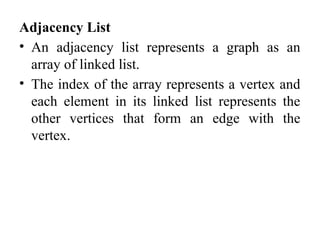
  • 45. The Bellman-Ford Algorithm Bellman-Ford(G, w, s) Initialize-Single-Source(G, s) for i := 1 to |V| - 1 do for each edge (u, v)  E do B-F(u, v, w) for each vertex v  u.adj do if d[v] > d[u] + w(u, v) then return False return True B-F(u, v, w) if d[v] > d[u] + w(u, v) then d[v] := d[u] + w(u, v) parent[v] := u
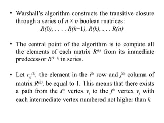
  • 46. Time Complexity Bellman-Ford(G, w, s) 1. Initialize-Single-Source(G, s) 2. for i := 1 to |V| - 1 do 3. for each edge (u, v)  E do 4. B-F(u, v, w) 5. for each vertex v  u.adj do 6. if d[v] > d[u] + w(u, v) 7. then return False // there is a negative cycle 8. return True O(|V|) O(|V||E|) O(|E|) Time complexity: O(|V||E|)
  • 47. Warshall’s Algorithm • It is named after Stephen Warshall. • It is used to constructs transitive closure of a directed graph. • The transitive closure of a directed graph with n vertices can be defined as the n×n boolean matrix T = {tij }, in which the element in the ith row and the jth column is 1 if there exists a nontrivial path from the ith vertex to the jth vertex; otherwise, tij is 0.
  • 48. • Warshall’s algorithm constructs the transitive closure through a series of n × n boolean matrices: R(0), . . . , R(k−1), R(k), . . . R(n) • The central point of the algorithm is to compute all the elements of each matrix R(k) from its immediate predecessor R(k−1) in series. • Let rij (k) , the element in the ith row and jth column of matrix R(k) , be equal to 1. This means that there exists a path from the ith vertex vi to the jth vertex vj with each intermediate vertex numbered not higher than k.
  • 49. Pseudocode ALGORITHM Warshall(A[1..n, 1..n]) //Implements Warshall’s algorithm for computing the //transitive closure //Input: The adjacency matrix A of a digraph with n vertices //Output: The transitive closure of the digraph R(0) ←A for k←1 to n do for i ←1 to n do for j ←1 to n do R(k) [i, j ] ← R(k−1) [i, j ] or (R(k−1) [i, k] and R(k−1) [k, j]) return R(n)
  • 50. • Time Efficiency : Ө (n3 ) • Space Efficiency: Matrices can be written over their predecessors
  • 51. Exercise • Apply Warshall’s algorithm to find the transitive closure of the digraph defined by the following adjacency matrix:
  • 52. Floyd’sAlgorithm • It also known as all-pairs shortest path • This algorithm is used to find the lengths of the shortest paths from each vertex to all other vertices in a weighted (directed/undirected) graph. • The lengths of shortest paths in an n×n matrix D is called the distance matrix. The element dij in the ith row and the jth column of this matrix indicates the length of the shortest path from the ith vertex to the jth vertex
  • 53. Pseudo Code ALGORITHM Floyd(W[1..n, 1..n]) //Implements Floyd’s algorithm for the all-pairs shortest-//paths problem //Input: The weight matrix W of a graph with no negative-//length cycle //Output: The distance matrix of the shortest paths’ //lengths D ←W //is not necessary if W can be overwritten for k←1 to n do for i ←1 to n do for j ←1 to n do D[i, j ]←min{D[i, j ], D[i, k]+ D[k, j]} return D
  • 54. Exercise Solve the all-pairs shortest-path problem for the digraph with the following weight matrix:
  • 55. Maximum-Flow Problem • The problem of maximizing the flow of a material through a transportation network • The transportation network can be represented by a connected weighted digraph with n vertices numbered from 1 to n and a set of edges E, with some properties.
  • 56. Properties are, • It contains exactly one vertex with no entering edges, this vertex is called the source • It contains exactly one vertex with no leaving edges, this vertex is called the sink • The weight uij of each directed edge (i, j) is a positive integer, called the edge capacity. A digraph satisfying these properties is called a flow network or network
  • 57. Flow-conservation requirement • The source and the sink are the only source and destination of the material respectively. All the other vertices serve only as points where a flow can be redirected without consuming material flow through it. • In other words, the total amount of the material entering an intermediate vertex must be equal to the total amount of the material leaving the vertex. This condition is called the flow-conservation requirement.
  • 58. • Flow Conservation: • The quantity of the total outflow from the source or equivalently, the total inflow into the sink is called the value of the flow.
  • 59. Ford-Fulkerson Method • Given a graph which represent a flow network where every edge has a capacity. Also given two vertices source ‘s’ and sink ‘t’ in a graph. • Find the maximum possible flow from s to t with some constraints, – Flow on an edge does not exceed the given capacity of the edge. – In-flow must be equal to out-flow for every vertex except source and sink.
  • 60. • Residual Network/Graph: It is a graph which indicates additional possible flow. If there is such path from source to sink then there is possibility to add the flow. • Residual Capacity It is the original capacity which represents capacity of edge minus flow.
  • 61. • Minimal Cut It is also known as bottle neck capacity, which decides maximum possible flow from source to sink through an augmented path. • Augmenting Path Augmenting path can classified as two types, Non-full forward edges Non-empty backward edges
  • 62. Algorithm • Initially Start with the flow value as 0. • While there is an augmenting path from source to sink, add that path flow value to flow. • Finally return the flow
  • 67. MAXIMUM MATCHING IN BIPARTITE GRAPHS • Bipartite graph: a graph whose vertices can be partitioned into two disjoint sets V and U, not necessarily of the same size, so that every edge connects a vertex in V to a vertex in U. • A graph is bipartite if and only if it does not have a cycle of an odd length.
  • 68. • A bipartite graph is 2-colorable: the vertices can be coloured in two colours so that every edge has its vertices coloured differently.
  • 69. Matching in a Graph • A matching in a graph is a subset of its edges with the property that no two edges share a vertex • A maximum (or maximum cardinality) matching is a matching with the largest number of edges
  • 70. Theorem: A matching M is maximum if and only if there exists no augmenting path with respect to M. • Start with some initial matching. e.g., the empty set • Find an augmenting path and augment the current matching along that path. e.g., using breadth-first search like method • When no augmenting path can be found, terminate and return the last matching, which is maximum