Unsupervised learning Algorithms and Assumptions

UNIT II
Unsupervised Learning
Dr. T. Veeramakali
Assoc. Prof. / DSBS
SRM Institute of Science & Technology
Kattankulathur, Chennai-603203.

Topics :
 Introduction to unsupervised learning
 Unsupervised learning Algorithms and Assumptions
 K-Means algorithm – introduction
 Implementation of K-means algorithm
 Hierarchical Clustering – need and importance of hierarchical clustering
 Agglomerative Hierarchical Clustering
 Working of dendrogram
 Steps for implementation of AHC using Python
 Gaussian Mixture Models – Introduction, importance and need of the model
 Normal , Gaussian distribution
 Implementation of Gaussian mixture model
 Understand the different distance metrics used in clustering
 Euclidean, Manhattan, Cosine, Mahala Nobis
 Features of a Cluster – Labels, Centroids, Inertia, Eigen vectors and Eigen
values
 Principal component analysis
Intro to Machine Learning
2

Supervised vs. Unsupervised Learning
 Supervised learning (classification)
 Supervision: The training data (observations,
measurements, etc.) are accompanied by labels
indicating the class of the observations
 New data is classified based on the training set
 Unsupervised learning (clustering)
 The class labels of training data is unknown
 Given a set of measurements, observations, etc. with
the aim of establishing the existence of classes or
clusters in the data

Issues: Data Preparation
 Data cleaning
 Preprocess data in order to reduce noise and handle
missing values
 Relevance analysis (feature selection)
 Remove the irrelevant or redundant attributes
 Data transformation
 Generalize and/or normalize data

Unsupervised Machine Learning
 Unsupervised Machine Learning is a technique that teaches machines to use
unlabeled or unclassified data.
 The idea is to expose computers to large volumes of varying data and allow
them to learn from that data to provide previously unknown insights and
identify hidden patterns.

 Unsupervised learning models utilize three main algorithms: clustering,
association, and dimensionality reduction.

 Clustering is the process of grouping similar entities together by categories.
 Unsupervised Machine Learning algorithms aim to find similarities in the data
points of the dataset and group them to give us insights into the underlying
patterns of different groups, for example, grouping documents by similar
topics.

Start with practical applications

What is Cluster Analysis?
 Cluster: a collection of data objects
 Similar to one another within the same cluster
 Dissimilar to the objects in other clusters
 Cluster analysis
 Finding similarities between data according to the
characteristics found in the data and grouping similar
data objects into clusters
 Unsupervised learning: no predefined classes
 Typical applications
 As a stand-alone tool to get insight into data distribution
 As a preprocessing step for other algorithms

Quality: What Is Good
Clustering?
 A good clustering method will produce high quality
clusters with
 high intra-class similarity
 low inter-class similarity
 The quality of a clustering result depends on both the
similarity measure used by the method and its
implementation
 The quality of a clustering method is also measured by its
ability to discover some or all of the hidden patterns

Measure the Quality of
Clustering
 Dissimilarity/Similarity metric: Similarity is expressed in
terms of a distance function, typically metric: d(i, j)
 There is a separate “quality” function that measures the
“goodness” of a cluster.
 The definitions of distance functions are usually very
different for interval-scaled, boolean, categorical, ordinal
ratio, and vector variables.
 Weights should be associated with different variables
based on applications and data semantics.
 It is hard to define “similar enough” or “good enough”
 the answer is typically highly subjective.

Typical Alternatives to Calculate the
Distance between Clusters
 Single link: smallest distance between an element in one cluster
and an element in the other, i.e., dis(Ki, Kj) = min(tip, tjq)
 Complete link: largest distance between an element in one cluster
and an element in the other, i.e., dis(Ki, Kj) = max(tip, tjq)
 Average: avg distance between an element in one cluster and an
element in the other, i.e., dis(Ki, Kj) = avg(tip, tjq)
 Centroid: distance between the centroids of two clusters, i.e.,
dis(Ki, Kj) = dis(Ci, Cj)
 Medoid: distance between the medoids of two clusters, i.e., dis(Ki,
Kj) = dis(Mi, Mj)
 Medoid: one chosen, centrally located object in the cluster

Centroid, Radius and Diameter of a
Cluster (for numerical data sets)
 Centroid: the “middle” of a cluster
N
t
N
i ip
m
C
)
(
1




Major Clustering Approaches (I)
 Partitioning approach:
 Construct various partitions and then evaluate them by some criterion,
e.g., minimizing the sum of square errors
 Typical methods: k-means, k-medoids, CLARANS
 Hierarchical approach:
 Create a hierarchical decomposition of the set of data (or objects) using
some criterion
 Typical methods: Diana, Agnes, BIRCH, ROCK, CAMELEON
 Density-based approach:
 Based on connectivity and density functions
 Typical methods: DBSACN, OPTICS, DenClue

Partitioning Algorithms: Basic Concept
 Partitioning method: Construct a partition of a database D of n objects
into a set of k clusters, s.t., min sum of squared distance
 Given a k, find a partition of k clusters that optimizes the chosen
partitioning criterion
 Global optimal: exhaustively enumerate all partitions
 Heuristic methods: k-means and k-medoids algorithms
 k-means (MacQueen’67): Each cluster is represented by the center
of the cluster
2
1 )
( mi
m
Km
t
k
m t
C
mi


 


K-Means Clustering-
 K-Means clustering is an unsupervised iterative clustering technique.
• It partitions the given data set into k predefined distinct clusters.
• A cluster is defined as a collection of data points exhibiting certain
similarities.
 It partitions the data set such that-
• Each data point belongs to a cluster with the nearest mean.
• Data points belonging to one cluster have high degree of similarity.
• Data points belonging to different clusters have high degree of
dissimilarity.
The K-Means Clustering Method

 Given k, the k-means algorithm is implemented in four
steps:
 Partition objects into k nonempty subsets
 Compute seed points as the centroids of the
clusters of the current partition (the centroid is the
center, i.e., mean point, of the cluster)
 Assign each object to the cluster with the nearest
seed point
 Go back to Step 2, stop when no more new
assignment

 Step 1: First, we need to provide the number of clusters, K, that need to
be generated by this algorithm.
 Step 2: Next, choose K data points at random and assign each to a
cluster. Briefly, categorize the data based on the number of data points.
 Step 3: The cluster centroids will now be computed.
 Step 4: Iterate the steps below until we find the ideal centroid, which is
the assigning of data points to clusters that do not vary.
 4.1 The sum of squared distances between data points and
centroids would be calculated first.
 4.2 At this point, we need to allocate each data point to the cluster
that is closest to the others (centroid).
 4.3 Finally, compute the centroids for the clusters by averaging all of
the cluster’s data points.

 K-means implements the Expectation-Maximization strategy to
solve the problem. The Expectation-step is used to assign data points to
the nearest cluster, and the Maximization-step is used to compute the
centroid of each cluster.
 When using the K-means algorithm, we must keep the
following points in mind:
 It is suggested to normalize the data while dealing with clustering
algorithms such as K-Means since such algorithms employ distance-
based measurement to identify the similarity between data points.
 Because of the iterative nature of K-Means and the random initialization
of centroids, K-Means may become stuck in a local optimum and fail to
converge to the global optimum. As a result, it is advised to employ
distinct centroids’ initializations.

Implementation of K Means Clustering
Graphical Form
 STEP 1: Let us pick k clusters, i.e., K=2, to separate the dataset and
assign it to its appropriate clusters. We will select two random places to
function as the cluster’s centroid.
 STEP 2: Now, each data point will be assigned to a scatter plot
depending on its distance from the nearest K-point or centroid. This will
be accomplished by establishing a median between both centroids.
Consider the following illustration:
 STEP 3: The points on the line’s left side are close to the blue centroid,
while the points on the line’s right side are close to the yellow centroid.
The left Form cluster has a blue centroid, whereas the right Form cluster
has a yellow centroid.
 STEP 4: Repeat the procedure, this time selecting a different centroid.
To choose the new centroids, we will determine their new center of
gravity, which is represented below:

Graphical Form
 STEP 5: After that, we’ll re-assign each data point to its new centroid. We shall
repeat the procedure outlined before (using a median line). The blue cluster will
contain the yellow data point on the blue side of the median line.
 STEP 6: Now that reassignment has occurred, we will repeat the previous step of
locating new centroids.

 STEP 7: We will repeat the procedure outlined above for determining the center
of gravity of centroids, as shown below.
 STEP 8: Similar to the previous stages, we will draw the median line and
reassign the data points after locating the new centroids.
Implementation of K Means Clustering Graphical
Form

 STEP 9: We will finally group points depending on their distance
from the median line, ensuring that two distinct groups are
established and that no dissimilar points are included in a single
group.
 The final Cluster is as follows:
Implementation of K Means Clustering Graphical
Form

 Example
0
1
2
3
4
5
6
7
8
9
10
0 1 2 3 4 5 6 7 8 9 10
0
1
2
3
4
5
6
7
8
9
10
0 1 2 3 4 5 6 7 8 9 10
0
1
2
3
4
5
6
7
8
9
10
0 1 2 3 4 5 6 7 8 9 10
0
1
2
3
4
5
6
7
8
9
10
0 1 2 3 4 5 6 7 8 9 10
0
1
2
3
4
5
6
7
8
9
10
0 1 2 3 4 5 6 7 8 9 10
K=2
Arbitrarily choose K
object as initial
cluster center
Assign
each
objects
to most
similar
center
Update
the
cluster
means
Update
the
cluster
means
reassign
reassign
Graphical Form

Distance Metrics
 Euclidean Distance represents the shortest distance between two
points.

The K-Means Clustering Problem
 Use K-Means Algorithm to create two clusters-

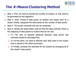
 Solution-
 Assume A(2, 2) and C(1, 1) are centers of the two clusters.
 Iteration-01:
 We calculate the distance of each point from each of the center of
the two clusters. The distance is calculated by using the euclidean
distance formula.
 The following illustration shows the calculation of distance between
point A(2, 2) and each of the center of the two clusters-

Calculating Distance Between A(2, 2) and
C1(2, 2)-
Ρ(A, C1)
= sqrt [ (x2 – x1)2 + (y2 – y1)2 ]
= sqrt [ (2 – 2)2 + (2 – 2)2 ]
= sqrt [ 0 + 0 ]
= 0
Calculating Distance Between A(2, 2)
and C2(1, 1)-
Ρ(A, C2)
= sqrt [ (x2 – x1)2 + (y2 – y1)2 ]
= sqrt [ (1 – 2)2 + (1 – 2)2 ]
= sqrt [ 1 + 1 ]
= sqrt [ 2 ]
= 1.41

 From here, New clusters are-
 Now, We re-compute the new cluster clusters.
 The new cluster center is computed by taking mean of all the points
contained in that cluster.
 This is completion of Iteration-01.
 Next, we go to iteration-02, iteration-03 and so on until the centers do not change
anymore.
Cluster-01:
First cluster contains points-
A(2, 2)
B(3, 2)
D(3, 1)
Cluster-02:
Second cluster contains points-
C(1, 1)
E(1.5, 0.5)

 Iteration-2
Given Points Distance from
centroid 1
(2.67,1.67)
Distance from
centroid 2
(1.25,0.75)
Point belongs
to cluster
A (2,2) 0.74 1.45 C1
B(3,2) 0.33 2.15 C1
C(1,1) 1.79 0.35 C2
D(3,1) 0.74 1.76 C1
E(1.5,0.5) 1.65 0.35 C2

Clustering: Rich Applications and
Multidisciplinary Efforts
 Pattern Recognition
 Spatial Data Analysis
 Create thematic maps in GIS by clustering feature
spaces
 Detect spatial clusters or for other spatial mining tasks
 Image Processing
 Economic Science (especially market research)
 WWW
 Document classification
 Cluster Weblog data to discover groups of similar access
patterns

Examples of Clustering
Applications
 Marketing: Help marketers discover distinct groups in their customer
bases, and then use this knowledge to develop targeted marketing
programs
 Land use: Identification of areas of similar land use in an earth
observation database
 Insurance: Identifying groups of motor insurance policy holders with
a high average claim cost
 City-planning: Identifying groups of houses according to their house
type, value, and geographical location
 Earth-quake studies: Observed earth quake epicenters should be
clustered along continent faults

Comments on the K-Means Method
 Strength: Relatively efficient: O(tkn), where n is # objects, k is #
clusters, and t is # iterations. Normally, k, t << n.
 Comment: Often terminates at a local optimum. The global optimum
may be found using techniques such as: deterministic annealing and
genetic algorithms
 Weakness
 Applicable only when mean is defined, then what about categorical
data?
 Need to specify k, the number of clusters, in advance
 Unable to handle noisy data and outliers
 Not suitable to discover clusters with non-convex shapes

Hierarchical Clustering
 In hierarchical clustering, we assign each object
(data point) to a separate cluster.
 Then compute the distance (similarity) between
each of the clusters and join the two most similar
clusters.
 Let’s say we have the below points and we want
to cluster them into groups:

 Let’s say we have the below points and we want
to cluster them into groups:
 We can assign each of these points to a separate
cluster:

 Now, based on the similarity of these clusters, we
can combine the most similar clusters together
and repeat this process until only a single cluster
is left:
 We are essentially building a hierarchy of clusters.
That’s why this algorithm is called hierarchical
clustering.

 Types of Hierarchical Clustering
 There are mainly two types of hierarchical
clustering:
 Agglomerative hierarchical clustering
 Divisive Hierarchical clustering

Agglomerative Hierarchical
Clustering
 We assign each point to an individual cluster in
this technique. Suppose there are 4 data points.
 We will assign each of these points to a cluster
and hence will have 4 clusters in the beginning:
 Then, at each iteration, we merge the closest pair
of clusters and repeat this step until only a single
cluster is left:

Divisive Hierarchical Clustering
 Divisive hierarchical clustering works in the opposite way. Instead of
starting with n clusters (in case of n observations), we start with a
single cluster and assign all the points to that cluster.
 Now, at each iteration, we split the farthest point in the cluster and
repeat this process until each cluster only contains a single point:
 We are splitting (or dividing) the clusters at each step, hence the
name divisive hierarchical clustering.

Agglomerative Hierarchical
Clustering - Example
 Suppose a teacher wants to divide her students into different groups.
 She has the marks scored by each student in an assignment and
based on these marks, she wants to segment them into groups.
 Let’s take a sample of 5 students:

Example
 Creating a Proximity Matrix:
 First, we will create a proximity matrix which will tell us the distance
between each of these points.
 Since we are calculating the distance of each point from each of the
other points, we will get a square matrix of shape n X n (where n is
the number of observations).
 Let’s make the 5 x 5 proximity matrix for our example:
 √(10-7)^2 = √9 = 3
 √(10-28)^2 = √324 = 18
 √(10-20)^2 = √100 = 10
 √(10-35)^2 = √625 = 25
 √(7-10)^2 = √9 = 3
 √(7-28)^2 = √441 = 21
 √(7-20)^2 = √169 = 13
 √(7-35)^2 = √784 = 28

Steps to Perform Hierarchical Clustering
 Step 1: First, we assign all the points to an individual cluster:
 Step 2: Next, we will look at the smallest distance in the proximity
matrix and merge the points with the smallest distance. We then
update the proximity matrix:
 Here, the smallest distance is 3 and hence we will merge point 1 and
2.

 Let’s look at the updated clusters and accordingly update the
proximity matrix:
 Max(7,10)=10
 Now, we will again calculate the proximity matrix for these clusters:

 Step 3: We will repeat step 2 until only a single cluster is left.
 So, we will first look at the minimum distance in the proximity matrix
and then merge the closest pair of clusters. We will get the merged
clusters as shown below after repeating these steps:

Working of dendrogram
A dendrogram is a diagram that shows the attribute distances between each pair
of sequentially merged classes.
To avoid crossing lines, the diagram is graphically arranged so that members of
each pair of classes to be merged are neighbors in the diagram.

Working of dendrogram
Step by step working of the algorithm:
Step-1: The data points P2 and P3 merged together and form a cluster,
correspondingly a dendrogram is created,.
Step-2: In the next step, P5 and P6 form a cluster, and the corresponding
dendrogram is created
Step-3: Again, two new dendrograms are formed that combine P1, P2, and P3 in one
dendrogram, and P4, P5, and P6, in another dendrogram.
Step-4: At last, the final dendrogram is formed that combines all the data points
together.

 To get the number of clusters for hierarchical clustering, we make use
of an awesome concept called a Dendrogram.
 A dendrogram is a tree-like diagram that records the sequences of
merges or splits.

 The number of clusters will be the number of vertical lines which are
being intersected by the line drawn using the threshold.
 In the above example, since the red line intersects 2 vertical lines, we
will have 2 clusters.
 One cluster will have a sample (1,2,4) and the other will have a
sample (3,5).

Gaussian Distribution
 A distribution in statistics is a function that shows
the possible values for a variable and how often
they occur.
 In probability theory and statistics, the Normal
Distribution, also called the Gaussian
Distribution.
 is the most significant continuous probability
distribution.
 Sometimes it is also called a bell curve.

Gaussian Distribution
Where,
x is the variable
μ is the mean
σ is the standard deviation
Normal distribution is the most used distribution in data science.
In a normal distribution graph, data is symmetrically distributed with no skew.
When plotted, the data follows a bell shape, with most values clustering around
a central region and tapering off as they go further away from the center.

 A Gaussian mixture model is a probabilistic model
that assumes all the data points are generated
from a mixture of a finite number of Gaussian
distributions with unknown parameters.
 One can think of mixture models as generalizing
k-means clustering to incorporate information
about the covariance structure of the data as well
as the centers of the latent Gaussians.


 Pros:
 Speed:It is the fastest algorithm for learning
mixture models
 Agnostic:As this algorithm maximizes only the
likelihood, it will not bias the means towards zero,
or bias the cluster sizes to have specific structures
that might or might not apply.

 Cons:
 Singularities: When one has insufficiently many points per
mixture, estimating the covariance matrices becomes
difficult, and the algorithm is known to diverge and find
solutions with infinite likelihood unless one regularizes the
covariances artificially.
 Number of components:This algorithm will always use all
the components it has access to, needing held-out data or
information theoretical criteria to decide how many
components to use in the absence of external cues.

Understand the different distance metrics
used in clustering
 A metric or distance function is a function d(x,y) d ( x , y ) that defines
the distance between elements of a set as a non-negative real
number.
 Distance metrics are a key part of several machine learning algorithms.
 These distance metrics are used in both supervised and unsupervised
learning, generally to calculate the similarity between data points.
 An effective distance metric improves the performance of our machine
learning model.

used in clustering
 to create clusters using a clustering algorithm such as K-Means Clustering or
k-nearest neighbor algorithm (knn)
 How will you define the similarity between different observations?
 How can we say that two points are similar to each other?
 This will happen if their features are similar, right?
 When we plot these points, they will be closer to each other by distance.

used in clustering
 how do we calculate this distance, and what are the different distance metrics
in machine learning?
 Also, are these metrics different for different learning problems?
 Do we use any special theorem for this?
 Types of Distance Metrics in Machine Learning
 Euclidean Distance
 Manhattan Distance
 Minkowski Distance
 Hamming Distance

used in clustering
Euclidean Distance
 Euclidean Distance represents the shortest distance between two vectors.
 It is the square root of the sum of squares of differences between
corresponding elements.

used in clustering
Euclidean Distance
 Formula for Euclidean Distance

used in clustering
Euclidean Distance
We can generalize this for an n-dimensional space as:
Where,
•n = number of dimensions
•pi, qi = data points

used in clustering
# importing the library
from scipy.spatial import distance
# defining the points
point_1 = (1, 2, 3)
point_2 = (4, 5, 6)
point_1, point_2
OUTPUT:
 ((1, 2, 3), (4, 5, 6))

used in clustering
# importing the library
from scipy.spatial import distance
# defining the points
point_1 = (1, 2, 3)
point_2 = (4, 5, 6)
point_1, point_2
# computing the euclidean distance
euclidean_distance = distance.euclidean(point_1, point_2)
print('Euclidean Distance b/w', point_1, 'and', point_2, 'is: ', euclidean_distance)
OUTPUT:
Euclidean Distance b/w (1, 2, 3) and (4, 5, 6) is: 5.196152422706632

used in clustering
Manhattan Distance
Manhattan Distance is the sum of absolute differences between points across all
the dimensions.
Formula for Manhattan Distance

used in clustering
Manhattan Distance
Manhattan Distance is the sum of absolute differences between points across all
the dimensions.
formula for an n-dimensional space is given as:
Where,
•n = number of dimensions
•pi, qi = data points

used in clustering
Manhattan Distance
manhattan_distance = distance.cityblock(point_1, point_2)
print('Manhattan Distance b/w', point_1, 'and', point_2, 'is: ',
manhattan_distance)
OUTPUT:
Manhattan Distance b/w (1, 2, 3) and (4, 5, 6) is: 9

used in clustering
Cosine
Cosine similarity is the cosine of the angle between the vectors;
that is, it is the dot product of the vectors divided by the product of their
lengths.
The cosine similarity is calculated as:
The cosine distance formula is then: 1 - Cosine Similarity

Cosine Distance & Cosine Similarity:
 Cosine distance & Cosine Similarity metric is
mainly used to find similarities between two data
points. As the cosine distance between the data
points increases, the cosine similarity, or the
amount of similarity decreases, and vice versa.
Thus, Points closer to each other are more similar
than points that are far away from each other.
Cosine similarity is given by Cos θ, and cosine
distance is 1- Cos θ. Example:-

In the above image, there are two data
points shown in blue, the angle between
these points is 90 degrees, and Cos 90 =
0. Therefore, the shown two points are not
similar, and their cosine distance is 1 —
Cos 90 = 1.

Now if the angle between the two points is
0 degrees in the above figure, then the
cosine similarity, Cos 0 = 1 and Cosine
distance is 1- Cos 0 = 0. Then we can
interpret that the two points are 100%
similar to each other.

In the above figure, imagine the value of θ
to be 60 degrees, then by cosine similarity
formula, Cos 60 =0.5 and Cosine distance
is 1- 0.5 = 0.5. Therefore the points are
50% similar to each other.

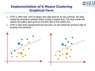
used in clustering
Cosine Distance:
Let's use an example to calculate the similarity between two fruits –
strawberries (vector A) and blueberries (vector B). Since our data is
already represented as a vector, we can calculate the distance.
Strawberry → [4,0,1]
Blueberry → [3,0,1]

The distance can be calculated using the below formula:-
Minkowski distance is a generalized distance metric.
We can manipulate the above formula by substituting ‘p’ to
calculate the distance between two data points in different ways.
Thus, Minkowski Distance is also known as Lp norm distance.
Some common values of ‘p’ are:-
•p = 1, Manhattan Distance
•p = 2, Euclidean Distance
•p = infinity, Chebychev Distance

Unsupervised learning Algorithms and Assumptions

used in clustering
Cosine Distance:

 Mahalanobis Distance is used for calculating the distance
between two data points in a multivariate space.
 Mahala Nobis distance takes covariance in account which
helps in measuring the strength/similarity between two
different data objects.
99
Mahalanobis Distance
Here, S is the covariance metrics. We are using inverse of the
covariance metric to get a variance-normalized distance
equation.

 In a regular Euclidean space, variables (e.g. x, y,
z) are represented by axes drawn at right angles
to each other;
 The distance between any two points can be
measured with a ruler.
 For uncorrelated variables, the Euclidean distance
equals the MD.
 However, if two or more variables are correlated,
the axes are no longer at right angles, and the
measurements become impossible with a ruler.

 In addition, if you have more than three variables,
you can’t plot them in regular 3D space at all.
 The MD solves this measurement problem, as it
measures distances between points, even
correlated points for multiple variables.

Mahalanobis distance plot example. A
contour plot overlaying the scatterplot of
100 random draws from a bivariate normal
distribution with mean zero, unit variance,
and 50% correlation. The centroid defined
by the marginal means is noted by a blue
square.

 The Mahalanobis distance measures distance
relative to the centroid — a base or central point
which can be thought of as an overall mean for
multivariate data.
 The centroid is a point in multivariate space where
all means from all variables intersect.
 The larger the MD, the further away from the
centroid the data point is.

 if the dimensions (columns in your dataset) are
correlated to one another, which is typically the case in
real-world datasets, the Euclidean distance between a
point and the center of the points (distribution) can
give little or misleading information about how close a
point really is to the cluster.

 Uses
 The most common use for the Mahalanobis
distance is to find multivariate outliers, which
indicates unusual combinations of two or more
variables. For example, it’s fairly common to find a
6′ tall woman weighing 185 lbs, but it’s rare to find
a 4′ tall woman who weighs that much.

 Inertia measures how well a dataset was clustered by K-
Means.
 It is calculated by measuring the distance between each
data point and its centroid, squaring this distance, and
summing these squares across one cluster.
 A good model is one with low inertia AND a low number of
clusters (K).
 However, this is a tradeoff because as K increases, inertia
decreases..
107
Inertia

 To find the optimal K for a dataset, use the Elbow method;
find the point where the decrease in inertia begins to slow.
 K=3 is the “elbow” of this graph.
108
Inertia

 It tells us how far the points within a cluster are.
So, inertia actually calculates the sum of distances of
all the points within a cluster from the centroid of that
cluster.
 Normally, we use Euclidean distance as the distance
metric, as long as most of the features are numeric;
otherwise, Manhattan distance in case most of the
features are categorical.
 We calculate this for all the clusters; the final inertial value
is the sum of all these distances. This distance within the
clusters is known as intracluster distance. So, inertia
gives us the sum of intracluster distances:

the distance between them should be as
low as possible.

Eigen vectors and Eigen values
 Eigenvalues and eigenvectors are concepts from
linear algebra that are used to analyze and
understand linear transformations, particularly
those represented by square matrices.
 They are used in many different areas of
mathematics, including machine learning and
artificial intelligence.
 used to determine a set of important variables (in
form of a vector) along with scale along different
dimensions (key dimensions based on variance)
for analyzing the data in a better manner.

 In machine learning, eigenvalues and eigenvectors are
used to represent data, to perform operations on
data, and to train machine learning models.
 In artificial intelligence, eigenvalues and eigenvectors
are used to develop algorithms for tasks such as
image recognition, natural language processing, and
robotics.
112

 Eigenvalues are the special set of scalar values that is
associated with the set of linear equations most probably in
the matrix equations.
 Eigenvectors are also termed as characteristic roots. It is a
non-zero vector that can be changed at most by its scalar
factor after the application of linear transformations.
 Av=λv
113

1. Eigenvalue (λ): An eigenvalue of a square matrix
A is a scalar (a single number) λ such that there
exists a non-zero vector v (the eigenvector) for
which the following equation holds:
Av = λv
In other words, when you multiply the matrix A by
the eigenvector v, you get a new vector that is
just a scaled version of v (scaled by the
eigenvalue λ).

 2. Eigenvector: The vector v mentioned above is
called an eigenvector corresponding to the
eigenvalue λ. Eigenvectors only change in
scale (magnitude) when multiplied by the
matrix A; their direction remains the same.
 Mathematically, to find eigenvalues and
eigenvectors, you typically solve the following
equation for λ and v:
 (A — λI)v = 0

(A — λI)v = 0
Where:
A is the square matrix for which you want to find
eigenvalues and eigenvectors.
λ is the eigenvalue you’re trying to find.
I is the identity matrix (a diagonal matrix with 1s on
the diagonal and 0s elsewhere).
v is the eigenvector you’re trying to find.

 Eigenvectors are the vectors that when
multiplied by a matrix (linear combination or
transformation) result in another vector having
the same direction but scaled (hence scaler
multiple) in forward or reverse direction by a
magnitude of the scaler multiple which can be
termed as

 Eigenvalue. In simpler words, the eigenvalues
are scalar values that represent the scaling factor
by which a vector is transformed when a linear
transformation is applied.
 In other words, eigenvalues are the values that
scale eigenvectors when a linear transformation is
applied.

When the matrix multiplication with
vector results in another vector in the
same/opposite direction but scaled in forward /
reverse direction by a magnitude of scaler multiple or
eigenvalue ,
then the vector is called the eigenvector of that matrix.
Here is the diagram representing the eigenvector x of
matrix A because the vector Ax is in the same/opposite
direction of x.

An eigenvector is a vector whose direction remains unchanged when a linear
transformation is applied to it. Consider the image below in which three vectors
are shown. The green square is only drawn to illustrate the linear transformation
that is applied to each of these three vectors.
Eigenvectors (red) do not change direction when a
linear transformation (e.g. scaling) is applied to
them. Other vectors (yellow) do.

Second Eigen value
We then arbitrarily choose , and find .
Therefore, the eigenvector that corresponds to eigenvalue is

Use of Eigenvalues and Eigenvectors
in Machine Learning and AI:
1. Dimensionality Reduction (PCA): In Principal
Component Analysis (PCA), you calculate the
eigenvectors and e¯igenvalues of the covariance matrix of
your datˀa. The eigenvectors (principal components) with
the largest eigenvalues capture the most variance in the
data and can be used to reduce the dimensionality of the
dataset while preserving important information.
2. Image Compression: Eigenvectors and eigenvalues are
used in techniques like Singular Value Decomposition
(SVD) for image compression. By representing images in
terms of their eigenvectors and eigenvalues, you can
reduce storage requirements while retaining essential
image features.

3. Support vector machines: Support vector
machines (SVMs) are a type of machine learning
algorithm that can be used for classification and
regression tasks. SVMs work by finding a
hyperplane that separates the data into two classes.
The eigenvalues and eigenvectors of the kernel
matrix of the SVM can be used to improve the
performance of the algorithm.
4. Graph Theory: Eigenvectors play a role in
analyzing networks and graphs. They can be used
to find important nodes or communities in social
networks or other interconnected systems.

5. Natural Language Processing (NLP): In NLP,
eigenvectors can help identify the most relevant
terms in a large document-term matrix, enabling
techniques like Latent Semantic Analysis (LSA) for
document retrieval and text summarization.
6. Machine Learning Algorithms: Eigenvalues and
eigenvectors can be used to analyze the stability
and convergence properties of machine learning
algorithms, especially in deep learning when dealing
with weight matrices in neural networks.

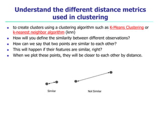
Example 1: Principal Component
Analysis (PCA)
 PCA is a widely used dimensionality reduction technique in machine
learning and data analysis.
 It employs eigenvectors and eigenvalues to reduce the number of
features while retaining as much information as possible.
 Imagine you have a dataset with two variables, X and Y, and you want
to reduce it to one dimension. You calculate the covariance matrix of
your data and find its eigenvectors and eigenvalues. Let’s say you
obtain the following:
• Eigenvalue 1 (λ₁) = 5
• Eigenvalue 2 (λ₂) = 1
• Eigenvector 1 (v₁) = [0.8, 0.6]
• Eigenvector 2 (v₂) = [-0.6, 0.8]
 In PCA, you would choose the eigenvector corresponding to the
largest eigenvalue as the principal component. In this case, it’s v₁. You
project your data onto this eigenvector to reduce it to one dimension,
effectively capturing most of the variance in the data.

 There are several key properties of eigenvalues and
eigenvectors that are important to understand. These
include:
1. Eigenvectors are non-zero vectors: Eigenvectors
cannot be zero vectors, as this would imply that the
transformation has no effect on the vector.
2. Eigenvalues can be real or complex: Eigenvalues can
be either real or complex numbers, depending on the
matrix being analyzed.
3. Eigenvectors can be scaled: Eigenvectors can be scaled
by any non-zero scalar value and still be valid eigenvectors.
4. Eigenvectors can be orthogonal: Eigenvectors that
correspond to different eigenvalues are always orthogonal
to each other.

 Principal component analysis (PCA) is a dimensionality
reduction and machine learning method used to simplify a
large data set into a smaller set.
 which is the process of reducing the number of predictor
variables in a dataset.
 PCA is an unsupervised type of feature extraction, where
original variables are combined and reduced to their most
important and descriptive components.
 The goal of PCA is to identify patterns in a data set, and
then distill the variables down to their most important
features so that the data is simplified without losing
important traits.
130
Principal component analysis

 PCA looks at the overall structure of the continuous
variables in a data set to extract meaningful signals from the
noise in the data set.
 It aims to eliminate redundancy in variables while preserving
important information.
131

 PCA originally hails from the field of linear algebra.
 It is a transformation method that creates (weighted linear)
combinations of the original variables in a data set, with the
intent that the new combinations will capture as
much variance (i.e., the separation between points) in the
dataset as possible while eliminating correlations (i.e.,
redundancy).
 PCA creates the new variables by transforming the original
(mean-centered) observations (records) in a dataset to a
new set of variables (dimensions) using the eigenvectors
and eigenvalues calculated from a covariance matrix of your
original variables.
132

Basic Terminologies of PCA
 Before getting into PCA, we need to understand
some basic terminologies,
• Variance – for calculating the variation of data
distributed across dimensionality of graph
• Covariance – calculating dependencies and
relationship between features
• Standardizing data – Scaling our dataset within
a specific range for unbiased output

in scaling, you're changing the range of your data
Normalization: in normalization you're changing the shape of
the distribution of your data. Data is transformed into a range
between 0 and 1 by normalization, which involves dividing a
vector by its length.
Standardization is divided by the standard deviation after the
mean has been subtracted.

 Covariance matrix – Used for
calculating interdependencies
between the features or
variables and also helps in
reduce it to improve the
performance
•Covariance matrix – Used for calculating
interdependencies between the features or variables and
also helps in reduce it to improve the performance

How does PCA work?
 The steps involved for PCA are as follows-
1. Original Data
2. Normalize the original data (mean =0, variance
=1)
3. Calculating covariance matrix
4. Calculating Eigen values, Eigen vectors, and
normalized Eigenvectors
5. Calculating Principal Component (PC)
6. Plot the graph for orthogonality between PCs

 A variance-covariance matrix is a square matrix
(has the same number of rows and columns) that
gives the covariance between each pair of
elements available in the data.
 Covariance measures the extent to which to
variables move in the same direction.

 A covariance matrix is:
• Symmetric
• The square matrix is equal to its transpose: 𝐴=𝐴𝑇.
• Positive semi-definite
• With main diagonal containing the variances
(covariances of variables on themselves)

variance-covariance-matrix-using-
python/
 Variance-Covariance Matrix Example
 First, let’s consider some sample data to work
with:
 Age Experience Salary
 0 25 2 2000
 1 32 6 3000
 2 37 9 3500

 https://www.turing.com/kb/guide-to-principal-
component-analysis
 https://pyshark.com/compute-variance-
covariance-matrix-using-python/

 Step 1: Standardization
 First, we need to standardize our dataset to ensure that
each variable has a mean of 0 and a standard deviation of
1.
 Here, μ is the mean of independent features

 σ is the standard deviation of independent features
147

 Step2: Covariance Matrix Computation
 Covariance measures the strength of joint variability
between two or more variables, indicating how much they
change in relation to each other. To find the covariance we
can use the formula:
 The value of covariance can be positive, negative, or zeros.
 Positive: As the x1 increases x2 also increases.
 Negative: As the x1 increases x2 also decreases.
 Zeros: No direct relation
148

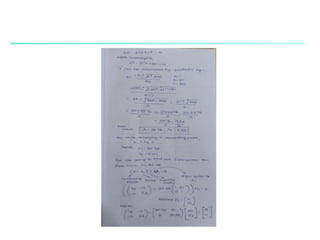
149

 How Principal Component Analysis(PCA) works?
import pandas as pd
import numpy as np
# Here we are using inbuilt dataset of scikit learn
from sklearn.datasets import load_breast_cancer
# instantiating
cancer = load_breast_cancer(as_frame=True)
# creating dataframe
df = cancer.frame
# checking shape
print('Original Dataframe shape :',df.shape)
# Input features
X = df[cancer['feature_names']]
print('Inputs Dataframe shape :', X.shape)
150

first calculate the mean and standard deviation of each feature in the feature space.
# Mean
X_mean = X.mean()
# Standard deviation
X_std = X.std()
# Standardization
Z = (X - X_mean) / X_std
151

The covariance matrix helps us visualize how strong the dependency of two features is with each other in
the feature space.
# covariance
c = Z.cov()
# Plot the covariance matrix
import matplotlib.pyplot as plt
import seaborn as sns
sns.heatmap(c)
plt.show()
152

Now we will compute the eigenvectors and eigenvalues for our feature space which serve a great purpose in
identifying the principal components for our feature space.
eigenvalues, eigenvectors = np.linalg.eig(c)
print('Eigen values:n', eigenvalues)
print('Eigen values Shape:', eigenvalues.shape)
print('Eigen Vector Shape:', eigenvectors.shape)
153

Sort the eigenvalues in descending order and sort the corresponding eigenvectors accordingly.
# Index the eigenvalues in descending order
idx = eigenvalues.argsort()[::-1]
# Sort the eigenvalues in descending order
eigenvalues = eigenvalues[idx]
# sort the corresponding eigenvectors accordingly
eigenvectors = eigenvectors[:,idx]
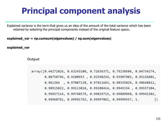
154

Explained variance is the term that gives us an idea of the amount of the total variance which has been
retained by selecting the principal components instead of the original feature space..
explained_var = np.cumsum(eigenvalues) / np.sum(eigenvalues)
explained_var
155

 Determine the Number of Principal Components
 Here we can either consider the number of principal components of any value of our choice or by
limiting the explained variance.
 Here considering explained variance more than equal to 50%.
 Let’s check how many principal components come into this.
n_components = np.argmax(explained_var >= 0.50) + 1
n_components
Output:
2
156

# PCA component or unit matrix
u = eigenvectors[:,:n_components]
pca_component = pd.DataFrame(u,
index = cancer['feature_names'],
columns = ['PC1','PC2']
)
# plotting heatmap
plt.figure(figsize =(5, 7))
sns.heatmap(pca_component)
plt.title('PCA Component')
plt.show()
157

# Matrix multiplication or dot Product
Z_pca = Z @ pca_component
# Rename the columns name
Z_pca.rename({'PC1': 'PCA1', 'PC2': 'PCA2'},
axis=1, inplace=True)
# Print the Pricipal Component values
print(Z_pca)
158

 The eigenvectors of the covariance matrix of the data are referred to as the
principal axes of the data, and the projection of the data instances onto these
principal axes are called the principal components.
 Dimensionality reduction is then obtained by only retaining those axes
(dimensions) that account for most of the variance, and discarding all others.
159

 PCA using Using Sklearn
 There are different libraries in which the whole process of the principal
component analysis has been automated by implementing it in a package
as a function and we just have to pass the number of principal components
which we would like to have. Sklearn is one such library that can be used
for the PCA as shown below.
# Importing PCA
from sklearn.decomposition import PCA
# Let's say, components = 2
pca = PCA(n_components=2)
pca.fit(Z)
x_pca = pca.transform(Z)
# Create the dataframe
df_pca1 = pd.DataFrame(x_pca,
columns=['PC{}'.
format(i+1)
for i in range(n_components)])
print(df_pca1)
160

 # giving a larger plot
 plt.figure(figsize=(8, 6))
 plt.scatter(x_pca[:, 0], x_pca[:, 1],
 c=cancer['target'],
 cmap='plasma')
 # labeling x and y axes
 plt.xlabel('First Principal Component')
 plt.ylabel('Second Principal Component')
 plt.show()
161

 # components
 pca.components_
162

Unsupervised learning Algorithms and Assumptions

Recommended

More Related Content

What's hot (20)

Similar to Unsupervised learning Algorithms and Assumptions (20)

Recently uploaded (20)

Unsupervised learning Algorithms and Assumptions