


![n개의 이전 단어 예측 단어
[1, 0, 0, 0, 0, 0, 0], [0, 1, 0, 0, 0, 0, 0],
[0, 0, 1, 0, 0, 0, 0], [0, 0, 0, 1, 0, 0, 0].
[0, 0, 0, 0, 1, 0, 0]
[0, 1, 0, 0, 0, 0, 0], [0, 0, 1, 0, 0, 0, 0]
[0, 0, 0, 1, 0, 0, 0], [0, 0, 0, 0, 1, 0, 0]
[0, 0, 0, 0, 0, 1, 0]
[0, 0, 1, 0, 0, 0, 0] [0, 0, 0, 1, 0, 0, 0],
[0, 0, 0, 0, 1, 0, 0], [0, 0, 0, 0, 0, 1, 0].
[0, 0, 0, 0, 0, 0, 1]
what will the fat cat sit on
what will the fat cat sit on
what will the fat cat sit on
예측할 다음 단어
이전 단어
window size=4. 앞의 단어 4개만을 참고
결과적으로 앞의 n개의 단어를 참고하는 셈이다.](https://image.slidesharecdn.com/deeplearningnlp-220122073423/85/PPT-Deep-Learning-for-Natural-Language-Processing-55-320.jpg)


![중심 단어 주변 단어
[1, 0, 0, 0, 0, 0, 0] [0, 1, 0, 0, 0, 0, 0], [0, 0, 1, 0, 0, 0, 0]
[0, 1, 0, 0, 0, 0, 0]
[1, 0, 0, 0, 0, 0, 0], [0, 0, 1, 0, 0, 0, 0],
[0, 0, 0, 1, 0, 0, 0]
[0, 0, 1, 0, 0, 0, 0]
[1, 0, 0, 0, 0, 0, 0], [0, 1, 0, 0, 0, 0, 0],
[0, 0, 0, 1, 0, 0, 0], [0, 0, 0, 0, 1, 0, 0]
[0, 0, 0, 1, 0, 0, 0]
[0, 1, 0, 0, 0, 0, 0], [0, 0, 1, 0, 0, 0, 0],
[0, 0, 0, 0, 1, 0, 0], [0, 0, 0, 0, 0, 1, 0]
[0, 0, 0, 0, 1, 0, 0]
[0, 0, 1, 0, 0, 0, 0], [0, 0, 0, 1, 0, 0, 0],
[0, 0, 0, 0, 0, 1, 0], [0, 0, 0, 0, 0, 0, 1]
[0, 0, 0, 0, 0, 1, 0]
[0, 0, 0, 1, 0, 0, 0], [0, 0, 0, 0, 1, 0, 0],
[0, 0, 0, 0, 0, 0, 1]
[0, 0, 0, 0, 0, 0, 1] [0, 0, 0, 0, 1, 0, 0], [0, 0, 0, 0, 0, 1, 0]
The fat cat sat on the mat
The fat cat sat on the mat
The fat cat sat on the mat
The fat cat sat on the mat
The fat cat sat on the mat
The fat cat sat on the mat
The fat cat sat on the mat
중심 단어
주변 단어
window size=2. 좌, 우 단어 2개씩을 참고.](https://image.slidesharecdn.com/deeplearningnlp-220122073423/85/PPT-Deep-Learning-for-Natural-Language-Processing-63-320.jpg)


![0.5 2.1 1.9 1.5
0.8 1.2 2.8 1.8
0.1 0.8 1.2 0.9
2.1 1.8 1.5 1.7
…
1.2 0.7 0.5 2.1
0.1 0.5 0.4 0.1
Word → Integer → lookup table → embedding vector
케라스의 embedding layer는 각 단어를 정수로 인코딩하고
이를 바탕으로 embedding layer를 사용하여 임베딩 벡터를 만든다.
본질적으로 lookup table이다.
위 embedding table은 모델의 학습 과정에서 값이 학습된다.
멋있어 1
최고야 2
짱이야 3
감탄이다 4
… …
최상의 14
퀄리티 15
['멋있어 최고야 짱이야 감탄이다', '헛소리 지껄이네', '닥쳐 자식아', '우와 대단하다', '우수한 성적', '형편없다', '
최상의 퀄리티']
를 정수로 인코딩하면
[[1, 2, 3, 4], [5, 6], [7, 8], [9, 10], [11, 12], [13], [14, 15]]
이제 여기에 embedding layer를 사용하면
0.5 2.1 1.9 1.5
단어 ‘멋있어’의
임베딩 벡터
훈련 과정에서 학습된다.](https://image.slidesharecdn.com/deeplearningnlp-220122073423/85/PPT-Deep-Learning-for-Natural-Language-Processing-81-320.jpg)


![LSTM LSTM LSTM
<sos> je suis
embedding embedding embedding
I am a student
LSTM LSTM LSTM LSTM
embedding embedding embedding embedding
dot product
ℎ1 ℎ2 ℎ3 ℎ4
𝑠𝑡−1
𝑇
Attention
Score
𝑒𝑡 = [𝑠𝑡−1
𝑇
ℎ1, . . . , 𝑠𝑡−1
𝑇
ℎ𝑁]
score(𝑠𝑡−1, ℎ𝑖) = 𝑠𝑡−1
𝑇
ℎ𝑖
1. 우선 어텐션 스코어를 구한다.](https://image.slidesharecdn.com/deeplearningnlp-220122073423/85/PPT-Deep-Learning-for-Natural-Language-Processing-140-320.jpg)


![BERT(12-layers)
Dense
[CLS] I love you
embedding
긍정 사람
BERT(12-layers)
[CLS] When Sebastian Thrun
embedding
Dense Dense Dense
X 사람
감성 분류 개체명 인식](https://image.slidesharecdn.com/deeplearningnlp-220122073423/85/PPT-Deep-Learning-for-Natural-Language-Processing-186-320.jpg)
![BERT(12-layers)
Dense
[CLS] I love you
embedding
Positive
[SEP]](https://image.slidesharecdn.com/deeplearningnlp-220122073423/85/PPT-Deep-Learning-for-Natural-Language-Processing-187-320.jpg)
![X
BERT(12-layers)
[CLS] Mike joined Aiimi
embedding
Dense Dense Dense
Person Organization
[SEP]
BERT(12-layers)](https://image.slidesharecdn.com/deeplearningnlp-220122073423/85/PPT-Deep-Learning-for-Natural-Language-Processing-188-320.jpg)
![BERT(12-layers)
[CLS] my dog is cute [SEP] he likes play ##ing [SEP]
Dense
True](https://image.slidesharecdn.com/deeplearningnlp-220122073423/85/PPT-Deep-Learning-for-Natural-Language-Processing-189-320.jpg)
![BERT(12-layers)
[CLS] Token1 [SEP] [SEP]
Label
Token2 Token3 Token4 Token5 Token6 Token7 Token8
Dense Dense Dense Dense](https://image.slidesharecdn.com/deeplearningnlp-220122073423/85/PPT-Deep-Learning-for-Natural-Language-Processing-190-320.jpg)
![BERT(12-layers)
[CLS] I love
love
입력 임베딩
출력 임베딩
[CLS] I you
you](https://image.slidesharecdn.com/deeplearningnlp-220122073423/85/PPT-Deep-Learning-for-Natural-Language-Processing-191-320.jpg)
![BERT(12-layers)
[CLS] I love you
love
BERT(12-layers)
[CLS] I love you
[CLS]
입력 임베딩
출력 임베딩](https://image.slidesharecdn.com/deeplearningnlp-220122073423/85/PPT-Deep-Learning-for-Natural-Language-Processing-192-320.jpg)
![[CLS] I love you
BERT Layer #1](https://image.slidesharecdn.com/deeplearningnlp-220122073423/85/PPT-Deep-Learning-for-Natural-Language-Processing-193-320.jpg)
![[CLS] I love you
BERT Layer #2
…
BERT Layer #12
Multi-head
Self-Attention
FFNN FFNN FFNN FFNN
Add & Norm
Add & Norm](https://image.slidesharecdn.com/deeplearningnlp-220122073423/85/PPT-Deep-Learning-for-Natural-Language-Processing-194-320.jpg)
![BERT(12-layers)
[CLS] I love you
0 1 2 3
+ + + +
Word Embedding
Position Embedding](https://image.slidesharecdn.com/deeplearningnlp-220122073423/85/PPT-Deep-Learning-for-Natural-Language-Processing-195-320.jpg)
![BERT(12-layers)
Dense
[CLS] I love you
embedding
긍정
BERT(12-layers)
Dense
[CLS] I love you
embedding
긍정](https://image.slidesharecdn.com/deeplearningnlp-220122073423/85/PPT-Deep-Learning-for-Natural-Language-Processing-196-320.jpg)
![BERT(12-layers)
[CLS] my dog is
0 1 2 3
+ + + +
WordPiece
Position
cute
4
+
[SEP] he likes play
5 6 7 8
+ + + +
##ing
9
+
[SEP]
10
+
0 0 0 0
+ + + +
0
+
0 1 1 1
+ + + +
1
+
1
+
Segment
Dense](https://image.slidesharecdn.com/deeplearningnlp-220122073423/85/PPT-Deep-Learning-for-Natural-Language-Processing-197-320.jpg)
![cat
BERT(12-layers)
[CLS] my [MASK] is cute [SEP] he likes play ##ing [SEP]
MLM
Classifier](https://image.slidesharecdn.com/deeplearningnlp-220122073423/85/PPT-Deep-Learning-for-Natural-Language-Processing-198-320.jpg)
![MLM
Classifier
BERT(12-layers)
[CLS] my [MASK] is cute [SEP] king likes play ##ing [SEP]
MLM
Classifier
MLM
Classifier](https://image.slidesharecdn.com/deeplearningnlp-220122073423/85/PPT-Deep-Learning-for-Natural-Language-Processing-199-320.jpg)
![MLM
Classifier
BERT(12-layers)
[CLS] my [MASK] is cute [SEP] king likes play ##ing [SEP]
MLM
Classifier
MLM
Classifier
NSP
Classifier](https://image.slidesharecdn.com/deeplearningnlp-220122073423/85/PPT-Deep-Learning-for-Natural-Language-Processing-200-320.jpg)
![BERT(12-layers)
[CLS] my dog is cute [SEP] [PAD] [PAD] [PAD] [PAD] [PAD]
Dense
1 1 1 1 1 1 0 0 0 0 0](https://image.slidesharecdn.com/deeplearningnlp-220122073423/85/PPT-Deep-Learning-for-Natural-Language-Processing-201-320.jpg)
![85.0%
12.0%
1.5% 1.5%
전체 단어
미사용
[MASK]로 변경 후 예측
랜덤으로 변경 후 예측
미변경 후 예측](https://image.slidesharecdn.com/deeplearningnlp-220122073423/85/PPT-Deep-Learning-for-Natural-Language-Processing-202-320.jpg)

![BERT(12-layers)
[CLS] I love
love
[CLS] I you
you
pooling
해당 문장의 표현 벡터](https://image.slidesharecdn.com/deeplearningnlp-220122073423/85/PPT-Deep-Learning-for-Natural-Language-Processing-204-320.jpg)


![[GomGuard] 뉴런부터 YOLO 까지 - 딥러닝 전반에 대한 이야기](https://cdn.slidesharecdn.com/ss_thumbnails/part1mlp2cnn-slidesharev-180308015531-thumbnail.jpg?width=560&fit=bounds)
![[우리가 데이터를 쓰는 법] 좋다는 건 알겠는데 좀 써보고 싶소. 데이터! - 넘버웍스 하용호 대표](https://cdn.slidesharecdn.com/ss_thumbnails/3-160416163055-thumbnail.jpg?width=560&fit=bounds)


![[DL輪読会]Batch Renormalization: Towards Reducing Minibatch Dependence in Batch-...](https://cdn.slidesharecdn.com/ss_thumbnails/dlu8f2au8aadu4f1av2-170407001546-thumbnail.jpg?width=560&fit=bounds)
![[226]대용량 텍스트마이닝 기술 하정우](https://cdn.slidesharecdn.com/ss_thumbnails/226-161025031656-thumbnail.jpg?width=560&fit=bounds)


![SSII2022 [TS1] Transformerの最前線〜 畳込みニューラルネットワークの先へ 〜](https://cdn.slidesharecdn.com/ss_thumbnails/ts120220608ssiitransformerr2-220607054025-3adacf07-thumbnail.jpg?width=560&fit=bounds)


![[야생의 땅: 듀랑고]의 식물 생태계를 담당하는 21세기 정원사의 OpenCL 경험담](https://cdn.slidesharecdn.com/ss_thumbnails/ndc2015-150521082100-lva1-app6891-thumbnail.jpg?width=560&fit=bounds)
Ad
More Related Content
What's hot (20)
Similar to 딥 러닝 자연어 처리 학습을 위한 PPT! (Deep Learning for Natural Language Processing) (20)


![[244] 분산 환경에서 스트림과 배치 처리 통합 모델](https://cdn.slidesharecdn.com/ss_thumbnails/244-150915025618-lva1-app6891-thumbnail.jpg?width=560&fit=bounds)


Ad
딥 러닝 자연어 처리 학습을 위한 PPT! (Deep Learning for Natural Language Processing)
- 1. 이 문서는 파워포인트로 자연어 처리의 여러 기법들을 이해하기 위한 ‘이미지’들을 만들어놓은 파일입니다. 발표용 자료가 아니므로 설명이 거의 없습니다. 각 페이지에 대한 설명은 오른쪽 하단 링크에 있습니다. 링크 : https://wikidocs.net/book/2155
- 2. LSA(Latent Semantic Analysis) 링크 : https://wikidocs.net/24949
- 3. 𝛴𝑡 𝑉𝑡 𝑇 Full SVD Truncated SVD = = 𝐴 𝑈 𝛴 𝑉𝑇 𝐴′ 𝑈𝑡 잠재 의미 분석(LSA)는 텍스트의 잠재된 의미를 도출하기 위해 차원 축소를 실행하는데, 이때 사용하는 것이 Truncated SVD이다. SVD(Singular Value Decomposition)
- 4. LDA(Latent Dirichlet Allocation) 링크 : https://wikidocs.net/30708
- 5. word apple banana apple dog dog topic B B ??? A A word cute book king apple apple topic B B B B B word apple banana apple dog dog topic B B ??? A A word cute book king apple apple topic B B B B B word apple banana apple dog dog topic B B ??? A A word cute book king apple apple topic B B B B B LDA 알고리즘은 모든 문서의 각 단어들에 대해서 루프를 돌리면서 토픽을 체크하고 업데이트합니다. 각 단어에 대해서 토픽은 아래의 두 가지 기준으로 할당됩니다. 1. How prevalent is that word across topics? 2. How prevalent are topics in the document? 1. How prevalent is that word across topics? ‘사과’라는 단어는 두 문서 전체에서 토픽 B의 약 절반을 차기합니다. 반면에, 토픽 A에서는 아무 지분도 차지하지 않습니다. 이 기준에 따르면 토픽 B에 할당될 가능성이 높 습니다. 2. How prevalent are topics in the document? Doc 1에서 토픽 A와 토픽 B는 50:50 비율입니다. 이 기준에 따르면 ‘사과'라는 단어는 절반의 확률을 가집니다. doc1 doc2 doc1 doc2 doc1 doc2
- 6. 코사인 유사도 : -1 코사인 유사도 : 0 코사인 유사도 : 1 코사인 유사도 링크 : https://wikidocs.net/24603
- 7. 통계 기반의 언어모델 링크 : https://wikidocs.net/21687
- 8. ) spreading is boy ( ) spreading is boy ( ) spreading is boy | ( Count Count P w w 통계적 언어 모델 An adorable little boy is spreading ? 무시됨! n-1개의 단어 N-gram 언어 모델
- 9. 머신 러닝 링크 : https://wikidocs.net/21679
- 10. 룰 베이스로 이미지 인식과 같은 문제를 풀고자하면? 규칙을 일일히 나열하는 것만으로는 해결 불가능한 문제들이 있다. (여기 고양이 사진은 현 PPT 공유자의 것이 아님.)
- 11. Data def predection(Data): ... program ... return 해답 해답 Data Data : 해답 1번 사진 : 강아지 2번 사진 : 고양이 3번 사진 : 강아지 4번 사진 : 고양이 5번 사진 : 강아지 ... 규칙성 해답 전통적인 프로그래밍의 접근 방법 머신 러닝의 접근 방법
- 12. 𝑥1 𝑥2 𝑥3 𝑥4 … 𝑥𝑛 𝑥1 𝑥2 𝑥3 𝑥4 … 𝑥𝑛 𝑥1 𝑥2 𝑥3 𝑥4 … 𝑥𝑛 𝑥1 𝑥2 𝑥3 𝑥4 … 𝑥𝑛 … … … … … … 𝑥1 𝑥2 𝑥3 𝑥4 … 𝑥𝑛 Sample-1 Sample-2 Sample-3 Sample-4 … Sample-m Feature-1 Feature-2 Feature-3 Feature-4 … Feature-n 머신 러닝 데이터셋에서 샘플(sample)과 특성(feature)의 개념 이해하기
- 13. 배포 수집 점검 및 탐색 머신 러닝 워크플로우 전처리 및 정제 모델링 및 훈련 평가 테스트 데이터 전체 데이터(Original Data) 훈련(Training) 테스트 (Testing) 테스트 (Testing) 훈련(Training) 검증 (Validation) 훈련 데이터와 검증 데이터의 분할
- 14. 선형 회귀와 경사 하강법 링크 : https://wikidocs.net/21670
- 16. cost W 접선의 기울기 = 0 cost W 접선의 기울기 = 0 ∂𝑐𝑜𝑠𝑡(𝑊) ∂𝑊 < 0 ∂𝑐𝑜𝑠𝑡(𝑊) ∂𝑊 > 0
- 17. 경사 하강법 SGD 배치 경사 하강법 vs. SGD
- 18. 로지스틱 회귀 링크 : https://wikidocs.net/22881
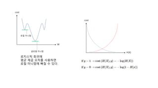
- 19. cost H(X) cost W 로컬 미니멈 글로벌 미니멈 로지스틱 회귀에 평균 제곱 오차를 사용하면 로컬 미니멈에 빠질 수 있다.
- 20. 소프트맥스 회귀 (다중 클래스 분류) -특성이 4개, 클래스가 3개 - iris data set으로 이해하기 링크 : https://wikidocs.net/35476
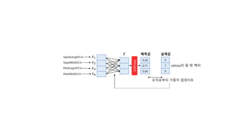
- 21. Softmax 𝑧1 SepalLengthCm SepalWidthCm PetalLegnthCm PetalWidthCm 𝑥1 𝑥2 𝑥3 𝑥4 소프트맥스 함수의 입력으로 어떻게 바꿀까? 오차를 어떻게 구할까? 예측값 1 : virginica 2 : setosa 3 : versicolor 화살표는 입력 데이터가 해당 품종일 확률 0.26 0.71 0.04
- 22. Softmax 𝑧1 SepalLengthCm SepalWidthCm PetalLegnthCm PetalWidthCm 0.26 0.71 0.04 𝑥1 𝑥2 𝑥3 𝑥4 오차 0 1 0 setosa의 원-핫 벡터 예측값 실제값 1 0 0 0 1 0 0 0 1 virginica의 원-핫 벡터 setosa의 원-핫 벡터 versicolor의 원-핫 벡터
- 23. Softmax 𝑧1 SepalWidthCm PetalLegnthCm PetalWidthCm 0.26 0.71 0.04 𝑥1 𝑥2 𝑥3 𝑥4 예측값 실제값 0 1 0 setosa의 원-핫 벡터 오차로부터 가중치 업데이트 SepalLengthCm
- 24. Softmax 𝑧1 SepalWidthCm PetalLegnthCm PetalWidthCm 0.26 0.71 0.04 𝑥1 𝑥2 𝑥3 𝑥4 예측값 실제값 0 1 0 setosa의 원-핫 벡터 오차로부터 가중치와 편향 업데이트 bias SepalLengthCm
- 25. 1 bias 𝑦1 𝑦2 … 𝑦𝑚 … 𝑥1 𝑥2 𝑥3 𝑥𝑛 현재 다룬 소프트맥스 회귀는 사실 얕은 인공 신경망으로도 볼 수 있다. Softmax 𝑧1 SepalWidthCm PetalLegnthCm PetalWidthCm 0.26 0.71 0.04 𝑥1 𝑥2 𝑥3 𝑥4 예측값 실제값 0 1 0 setosa의 원-핫 벡터 오차로부터 가중치와 편향 업데이트 bias SepalLengthCm
- 26. softmax ( ) × = 예측값𝑡 c × 1 𝑥1 𝑊 𝑥 + 𝑏 c × 1 f × 1 c × f 소프트맥스 회귀를 벡터와 행렬 연산으로 표현하면? f : 특성(feature)의 수 c : 클래스(class)의 수
- 29. 출력층(output layer) … 입력층(input layer) 1 bias 𝑥1 𝑥2 𝑥3 𝑥𝑛 … 𝑊1 𝑊2 𝑊3 𝑊 𝑛 𝑦 이 두 개의 층을 입력층과 출력층이라고 부른다.
- 30. 𝒙𝟏 𝒙𝟐 (0,1) (0,0) (1,0) (1,1) OR GATE 𝒙𝟏 𝒙𝟐 (0,1) (0,0) (1,0) (1,1) NAND GATE 𝒙𝟏 𝒙𝟐 𝒚 0 0 0 0 1 1 1 0 1 1 1 1 𝒙𝟏 𝒙𝟐 𝒚 0 0 1 0 1 1 1 0 1 1 1 0 퍼셉트론으로 OR 게이트와 NAND 게이트를 구현할 수 있다.
- 31. 𝒙𝟏 𝒙𝟐 𝒚 0 0 0 0 1 0 1 0 0 1 1 1 𝒙𝟏 𝒙𝟐 (0,1) (0,0) (1,0) (1,1) AND GATE 𝒙𝟏 𝒙𝟐 𝒚 0 0 0 0 1 1 1 0 1 1 1 0 𝒙𝟏 𝒙𝟐 (0,1) (0,0) (1,0) (1,1) ? XOR GATE 퍼셉트론으로 AND 게이트를 구현할 수 있지만 XOR 게이트는?
- 32. 𝒙𝟏 𝒙𝟐 (0,1) (0,0) (1,0) (1,1) XOR GATE 초기 퍼셉트론의 한계인 XOR 문제
- 33. 은닉층(hidden layer) 출력층 입력층 NAND OR AND 1 1 bias bias 𝑥1 𝑥2 𝑠1 𝑠2 𝑦 1 다층 퍼셉트론의 등장으로 XOR 문제를 해결하였다.
- 34. 은닉층(hidden layer) 출력층(output layer) 입력층(input layer) … … … 은닉층을 좀 더 추가하면 신경망이 깊어진다.
- 35. … … … 1 bias 1 bias 1 bias 은닉층(hidden layer) 출력층(output layer) 입력층(input layer) 은닉층을 좀 더 추가하면 신경망이 깊어진다. bias 추가한 그림.
- 36. 은닉층(hidden layer) 출력층(output layer) 입력층(input layer) … … … 각 층과 이름을 부각시킨 그림.
- 37. 다양한 인공 신경망 (얕은 신경망, 깊은 신경망, RNN) 링크 : https://wikidocs.net/24987
- 38. 𝑥2 𝑊2 입력층(input layer) 출력층(output layer) 𝑥1 𝑥3 𝑊1 𝑊3 𝑦1 입력층(input layer) 은닉층(hidden layer) y1 𝑥4 y1 𝑠3 𝑠1 𝑠2 𝑠4 y1 y1 𝑠7 𝑠5 𝑠6 𝑠8 𝑦1 출력층(output layer) 𝑥2 𝑥1 𝑥3 단층 퍼셉트론 다층 퍼셉트론 은닉층이 2개 미만인 신경망은 얕은 신경망(Shallow Neural Network)
- 39. y1 y1 y1 y1 은닉층이 2개인 다층 퍼셉트론. 은닉층이 2개 이상이므로 DNN(Deep Neural Network)! 이걸 학습하면 딥 러닝(Deep Learning)!
- 40. 순방향 신경망(Feed-Forward Neural Network) (또는 피드 포워드 신경망이라고도 한다.) 순환 신경망(Recurrent Neural Network) Vs. RNN(순환 신경망)은 은닉층에 사이클이 존재하는 신경망이라는 점에서 앞서 본 신경망들과 다르다.
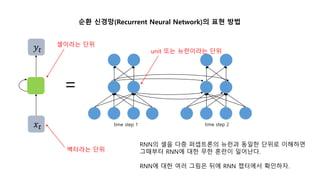
- 41. 순환 신경망(Recurrent Neural Network)의 표현 방법 time step 1 time step 2 = 𝑥𝑡 𝑦𝑡 unit 또는 뉴런이라는 단위 셀이라는 단위 벡터라는 단위 RNN의 셀을 다층 퍼셉트론의 뉴런과 동일한 단위로 이해하면 그때부터 RNN에 대한 무한 혼란이 일어난다. RNN에 대한 여러 그림은 뒤에 RNN 챕터에서 확인하자.
- 42. 인공신경망의 학습 링크 : https://wikidocs.net/36033
- 43. 200 200 200 200 200 200 200 200 200 200 Total data : 2,000 Batch size : 200 Iteration : 10 + 1 epoch Epoch와 batch size와 iteration의 관계 𝑋𝑚 x 𝑛 × 𝑊? x ? + 𝐵? x ? = 𝑌𝑚 x 𝑗 𝑋𝑚 x 𝑛 × 𝑊𝑛 x ? + 𝐵𝑚 x 𝑗 = 𝑌𝑚 x 𝑗 같아야 한다 𝑋𝑚 x 𝑛 × 𝑊? x ? + 𝐵𝑚 x 𝑗 = 𝑌𝑚 x 𝑗 같아야 한다 𝑋𝑚 x 𝑛 × 𝑊𝑛 x 𝑗 + 𝐵𝑚 x 𝑗 = 𝑌𝑚 x 𝑗 같아야 한다 인공 신경망의 가중치 행렬과 편향 행렬의 크기 계산
- 44. … … … 가중치 가중치 가중치 예측값 순전파(Forward Propagation)
- 45. 출력층(output layer) 입력층(input layer) … … … 가중치 가중치 가중치 예측값 실제값(레이블) 손실 함수(Loss function) 옵티마이저 (역전파 과정) 가중치 업데이트
- 46. … … … 예측값 실제값(레이블) 손실 함수(Loss function) 옵티마이저 (역전파 과정) 가중치 업데이트 가중치 가중치 가중치 역전파(Back Propagation)
- 47. 실제 계산 예제로 이해하는 역전파 설명 : https://wikidocs.net/37406
- 48. 𝑜1 𝑜2 ℎ1 ℎ2 𝑥1 𝑥2 𝑊1 𝑊2 𝑊4 𝑊3 𝑊5 𝑊6 𝑊8 𝑊7 𝑧1 𝑧2 𝑧3 𝑧4 1 1 𝑏1 𝑏2 역전파(Back Propagation) 𝑜1 𝑜2 ℎ1 ℎ2 𝑥1 𝑥2 𝑊1 𝑊2 𝑊4 𝑊3 𝑊5 𝑊6 𝑊8 𝑊7 𝑧1 𝑧2 𝑧3 𝑧4 1 1 𝑏1 𝑏2 역전파(Back Propagation) .1 .2 .3 .25 .4 .35 .45 .4 .7 .6 .15 .2 실제값 : 0.4 실제값 : 0.6 bias도 있는 경우
- 49. 𝑜1 𝑜2 ℎ1 ℎ2 𝑥1 𝑥2 𝑊1 𝑊2 𝑊4 𝑊3 𝑊5 𝑊6 𝑊8 𝑊7 𝑧1 𝑧2 𝑧3 𝑧4 𝑜1 𝑜2 ℎ1 ℎ2 𝑥1 𝑥2 𝑊1 𝑊2 𝑊4 𝑊3 𝑊5 𝑊6 𝑊8 𝑊7 𝑧1 𝑧2 𝑧3 𝑧4 .1 역전파(Back Propagation) 역전파(Back Propagation) .2 .3 .25 .4 .35 .45 .4 .7 .6 실제값 : 0.4 실제값 : 0.6 𝑜1 𝑜2 ℎ1 ℎ2 𝑥1 𝑥2 𝑊1 𝑊2 𝑊4 𝑊3 𝑊5 𝑊6 𝑊8 𝑊7 𝑧1 𝑧2 𝑧3 𝑧4 𝑜1 𝑜2 ℎ1 ℎ2 𝑥1 𝑥2 𝑊1 𝑊2 𝑊4 𝑊3 𝑊5 𝑊6 𝑊8 𝑊7 𝑧1 𝑧2 𝑧3 𝑧4 가중치 업데이트 완료 bias를 배제한 경우
- 50. 드롭아웃
- 52. 다양한 단어의 표현 방법 링크 : https://wikidocs.net/31767
- 53. Word Representation Local Representation Continuous Representation Count Based One-hot Vector Bag of Words (DTM, TF-IDF) N-gram Count Based Prediction Based Full Document LSA, LDA Windows GloVe Word2Vec (FastText)
- 54. NNLM (Neural Network Language Model) N-gram 언어 모델의 sparsity problem을 해결하기 위해 인공 신경망 언어 모델 NNLM이 제안되다. 이 NNLM은 향후 Word2Vec으로 발전한다. 링크 : https://wikidocs.net/45609 인공 신경망 언어 모델의 등장!
- 55. n개의 이전 단어 예측 단어 [1, 0, 0, 0, 0, 0, 0], [0, 1, 0, 0, 0, 0, 0], [0, 0, 1, 0, 0, 0, 0], [0, 0, 0, 1, 0, 0, 0]. [0, 0, 0, 0, 1, 0, 0] [0, 1, 0, 0, 0, 0, 0], [0, 0, 1, 0, 0, 0, 0] [0, 0, 0, 1, 0, 0, 0], [0, 0, 0, 0, 1, 0, 0] [0, 0, 0, 0, 0, 1, 0] [0, 0, 1, 0, 0, 0, 0] [0, 0, 0, 1, 0, 0, 0], [0, 0, 0, 0, 1, 0, 0], [0, 0, 0, 0, 0, 1, 0]. [0, 0, 0, 0, 0, 0, 1] what will the fat cat sit on what will the fat cat sit on what will the fat cat sit on 예측할 다음 단어 이전 단어 window size=4. 앞의 단어 4개만을 참고 결과적으로 앞의 n개의 단어를 참고하는 셈이다.
- 56. will(one-hot vector) the(one-hot vector) fat(one-hot vector) cat(one-hot vector) sit(one-hot vector) Projection layer (linear) Hidden layer (nonlinear) Output layer Input layer NNLM(2003)은 총 4개의 layer로 구성된다. n × V n × m 500 < h < 1000 (typically) V
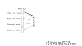
- 57. Input layer 우선 Projection layer 단계에서는 각 원-핫 벡터는 테이블 룩업을 진행한다. will(one-hot vector) the(one-hot vector) fat(one-hot vector) cat(one-hot vector)
- 58. 0.5 2.1 1.9 1.5 0.8 0.8 1.2 2.8 1.8 2.1 0.1 0.8 1.2 0.9 0.7 2.1 1.8 1.5 1.7 2.7 0 0 0 1 0 0 0 × = 2.1 1.8 1.5 1.7 2.7 lookup table 𝑥𝑓𝑎𝑡 × 𝑊𝑉×𝑀 = 𝑒𝑓𝑎𝑡 테이블 룩-업이란? V가 vocabular의 크기, M을 embedding vecto의 차원이면 원-핫 벡터가 V x M 행렬을 곱해서 더 작은 차원의 벡터가 된다.
- 59. Input layer Projection layer (linear) concatenate n × V n × m 테이블 룩-업으로 차원이 축소된 각 단어 벡터들이 모두 연결이 되면 projection layer의 결과물이다. will(one-hot vector) the(one-hot vector) fat(one-hot vector) cat(one-hot vector)
- 60. Projection layer (linear) Hidden layer (nonlinear) Input layer n × m h will(one-hot vector) the(one-hot vector) fat(one-hot vector) cat(one-hot vector)
- 61. Hidden layer (nonlinear) sit(one-hot vector) 0 0 0 0 0 1 0 0.1 0.03 0.02 0.05 0.01 0.7 0.09 𝑦𝑝𝑟𝑒𝑑𝑖𝑐𝑡𝑒𝑑 cross entropy Output layer Projection layer (linear) Input layer will(one-hot vector) the(one-hot vector) fat(one-hot vector) cat(one-hot vector) h V 𝑦 NNLM은 희소 문제(Data Sparsity) 문제를 해결했지만 N-gram 언어 모델과 마찬가지로 앞의 n개의 단어만을 참고한다는 문제가 있다.
- 62. Word2Vec 링크 : https://wikidocs.net/22660 NNLM이 발전되어 단어 임베딩 그 자체에 집중한 Word2Vec이 등장한다.
- 63. 중심 단어 주변 단어 [1, 0, 0, 0, 0, 0, 0] [0, 1, 0, 0, 0, 0, 0], [0, 0, 1, 0, 0, 0, 0] [0, 1, 0, 0, 0, 0, 0] [1, 0, 0, 0, 0, 0, 0], [0, 0, 1, 0, 0, 0, 0], [0, 0, 0, 1, 0, 0, 0] [0, 0, 1, 0, 0, 0, 0] [1, 0, 0, 0, 0, 0, 0], [0, 1, 0, 0, 0, 0, 0], [0, 0, 0, 1, 0, 0, 0], [0, 0, 0, 0, 1, 0, 0] [0, 0, 0, 1, 0, 0, 0] [0, 1, 0, 0, 0, 0, 0], [0, 0, 1, 0, 0, 0, 0], [0, 0, 0, 0, 1, 0, 0], [0, 0, 0, 0, 0, 1, 0] [0, 0, 0, 0, 1, 0, 0] [0, 0, 1, 0, 0, 0, 0], [0, 0, 0, 1, 0, 0, 0], [0, 0, 0, 0, 0, 1, 0], [0, 0, 0, 0, 0, 0, 1] [0, 0, 0, 0, 0, 1, 0] [0, 0, 0, 1, 0, 0, 0], [0, 0, 0, 0, 1, 0, 0], [0, 0, 0, 0, 0, 0, 1] [0, 0, 0, 0, 0, 0, 1] [0, 0, 0, 0, 1, 0, 0], [0, 0, 0, 0, 0, 1, 0] The fat cat sat on the mat The fat cat sat on the mat The fat cat sat on the mat The fat cat sat on the mat The fat cat sat on the mat The fat cat sat on the mat The fat cat sat on the mat 중심 단어 주변 단어 window size=2. 좌, 우 단어 2개씩을 참고.
- 64. fat(one-hot vector) cat(one-hot vector) on(one-hot vector) the(one-hot vector) sat(one-hot vector) Output layer Projection layer Input layer Word2Vec은 총 3개의 layer로 구성된다. 가운데 층을 hidden layer라고 하는 그림도 있지만 중요한 건 은닉층에 활성화 함수가 없다는 것이다. 이를 일반적인 은닉층과 구분하기 위해 projection layer라고도 부른다.
- 65. cat(one-hot vector) on(one-hot vector) sat(one-hot vector) 0 0 0 1 0 0 0 0 0 0 0 1 0 0 0 0 1 0 0 0 0 𝑊𝑉×𝑀 𝑊𝑉×𝑀 𝑊′𝑀×𝑉 M Projection layer Output layer Input layer
- 66. 0.5 2.1 1.9 1.5 0.8 0.8 1.2 2.8 1.8 2.1 2.1 1.8 1.5 1.7 2.7 0 0 1 0 0 0 0 × = 2.1 1.8 1.5 1.7 2.7 lookup table 𝒙𝒄𝒂𝒕 × 𝑾𝑽×𝑴 = 𝑽𝒄𝒂𝒕 cat(one-hot vector) on(one-hot vector) sat(one-hot vector) 0 0 0 1 0 0 0 0 0 0 0 1 0 0 0 0 1 0 0 0 0 𝑊′𝑀×𝑉 M
- 67. cat(one-hot vector) on(one-hot vector) sat(one-hot vector) 0 0 0 1 0 0 0 0 0 0 0 1 0 0 0 0 1 0 0 0 0 fat(one-hot vector) the(one-hot vector) 𝒗 = 𝑽𝒇𝒂𝒕 + 𝑽𝒄𝒂𝒕 + 𝑽𝒐𝒏 + 𝑽𝒕𝒉𝒆 𝟐×𝒏(𝒘𝒊𝒏𝒐𝒘 𝒔𝒊𝒛𝒆) M
- 68. cat(one-hot vector) on(one-hot vector) 0 0 0 0 1 0 0 0 0 1 0 0 0 0 𝑾′𝑴×𝑽× 𝒗 = 𝒛 𝒚 = 𝒔𝒐𝒇𝒕𝒎𝒂𝒙(𝒛) sat(one-hot vector) 0 0 0 1 0 0 0 0.1 0.03 0.02 0.7 0.01 0.05 0.09 cross entropy Output layer V 𝑦𝑝𝑟𝑒𝑑𝑖𝑐𝑡𝑒𝑑 𝑦 M
- 69. fat(one-hot vector) cat(one-hot vector) on(one-hot vector) the(one-hot vector) sat(one-hot vector) Output layer Projection layer Input layer Skip-gram
- 70. NNLM vs Word2Vec 링크 : https://wikidocs.net/22660 NNLM이 발전되어 Word2Vec이 등장한다.
- 71. Input layer Projection layer Hidden layer Output layer V n × m V n × m h Feed forward NNLM Word2Vec(CBOW) n : 학습에 사용되는 단어의 수 m : 임베딩 벡터의 크기 h : 은닉층의 크기 V : 단어 집합의 크기
- 73. 중심 단어 주변 단어 cat The cat Fat cat sat cat on sat fat sat cat sat on sat the The fat cat sat on the mat The fat cat sat on the mat 중심 단어 주변 단어 window size=2. 좌, 우 단어 2개씩을 참고.
- 74. sat The fat cat sat on the mat 중심 단어 주변 단어 cat sat Skip-gram Skip-gram (Negative Sampling) 0.88 cat
- 75. 입력 레이블 cat The cat fat cat sat cat on sat fat sat cat sat on sat the … … The fat cat sat on the mat The fat cat sat on the mat 중심 단어 주변 단어 입력1 입력2 레이블 cat The 1 cat fat 1 cat sat 1 cat on 1 sat fat 1 sat cat 1 sat on 1 sat the 1 … … … 입력과 레이블의 변화
- 76. 입력1 입력2 레이블 cat The 1 cat fat 1 cat sat 1 cat on 1 입력1 입력2 레이블 cat The 1 cat fat 1 cat pizza 0 cat computer 0 cat sat 1 cat on 1 단어 집합에서 랜덤으로 선택된 단어들을 레이블 0의 샘플로 추가. Negative Sampling 입력과 레이블의 변화
- 77. 입력1 입력2 레이블 cat The 1 cat fat 1 cat pizza 0 cat computer 0 cat sat 1 cat on 1 cat cute 1 cat mighty 0 … … … Embedding layer Embedding layer
- 78. Embedding layer Embedding layer cat The fat pizza
- 79. cat The fat pizza ⋅ Embedding layer Embedding layer cat The fat pizza = 0.55 1 = 0.88 1 = 0.45 0 예측값 레이블 Error 임베딩 벡터 업데이트!
- 80. 딥 러닝 프레임워크에서의 임베딩 층(Embedding layer) 링크 : https://wikidocs.net/33793
- 81. 0.5 2.1 1.9 1.5 0.8 1.2 2.8 1.8 0.1 0.8 1.2 0.9 2.1 1.8 1.5 1.7 … 1.2 0.7 0.5 2.1 0.1 0.5 0.4 0.1 Word → Integer → lookup table → embedding vector 케라스의 embedding layer는 각 단어를 정수로 인코딩하고 이를 바탕으로 embedding layer를 사용하여 임베딩 벡터를 만든다. 본질적으로 lookup table이다. 위 embedding table은 모델의 학습 과정에서 값이 학습된다. 멋있어 1 최고야 2 짱이야 3 감탄이다 4 … … 최상의 14 퀄리티 15 ['멋있어 최고야 짱이야 감탄이다', '헛소리 지껄이네', '닥쳐 자식아', '우와 대단하다', '우수한 성적', '형편없다', ' 최상의 퀄리티'] 를 정수로 인코딩하면 [[1, 2, 3, 4], [5, 6], [7, 8], [9, 10], [11, 12], [13], [14, 15]] 이제 여기에 embedding layer를 사용하면 0.5 2.1 1.9 1.5 단어 ‘멋있어’의 임베딩 벡터 훈련 과정에서 학습된다.
- 82. RNN(순환 신경망) 링크 : https://wikidocs.net/22886
- 83. … = 𝑥𝑡 𝑦𝑡 Cell 𝑥𝑡 𝑥1 𝑥2 𝑥3 𝑥𝑡 𝑦𝑡 𝑦1 𝑦2 𝑦3 𝑦𝑡 아래의 RNN은 기본적으로 입, 출력이 벡터로 가정되고 있다.
- 84. 일 대 다(one-to-many) 다 대 일(many-to-one) 다 대 다(many-to-many)
- 85. claim your winning 스팸 메일 x2 y2 prize 스팸 메일 분류 다 대 일(many-to-one) 구조의 RNN
- 86. EU rejects GERMAN 조직이름 해당없음 나라이름 해당없음 x2 y2 call 개체명 인식 다 대 다(many-to-many) 구조의 RNN
- 88. tanh ( ) × = ℎ𝑡 𝐷ℎ× 1 𝑥𝑡 𝑊 𝑥 × 𝑊ℎ ℎ𝑡−1 + + 𝑏 𝐷ℎ× 1 𝐷ℎ× 1 d × 1 𝐷ℎ× d 𝐷ℎ× 𝐷ℎ RNN을 벡터와 행렬 연산으로 표현하면? d : t time-step의 단어의 차원 𝐷ℎ : hidden size의 크기
- 89. … 𝑥1 𝑥2 𝑥3 𝑥𝑡 𝑦1 𝑦2 𝑦3 𝑦𝑡 깊은 RNN
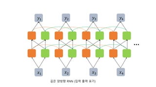
- 90. 𝑦1 𝑦2 𝑦3 𝑦4 𝑥1 𝑥2 𝑥3 𝑥4 양방향 RNN. 출력을 결정할 때마다 앞의 단어들만 보지말고 뒤의 단어들도 보자.
- 91. 깊은 양방향 RNN (은닉층이 2개)
- 92. … 𝑦2 𝑦3 𝑦4 𝑥1 𝑥2 𝑥3 𝑥4 깊은 양방향 RNN (입력 출력 표기) 𝑦1
- 93. No. of samples = batch_size input_length = timeseries = timesteps input_dim = Dimensionality of word representation RNN의 입출력 이해를 위해서는 3D 텐서를 이해해야한다.
- 94. 11 0 5 82 99 -8 3 4 78 1 43 28 51 7 32 -2 99 0 31 83 5 11 11 0 5 82 99 -8 3 4 78 1 43 28 11 0 5 82 99 -8 3 4 78 1 43 28 11 0 5 82 99 -8 3 4 78 1 43 28 SCALAR VECTOR MATRIX 3D TENSOR/CUBE 4D TENSOR VECTOR OF CUBES 5D TENSOR MATRIX OF CUBES 다양한 텐서
- 95. 𝑦𝑡 𝑤𝑦 𝑤𝑥 𝑥𝑡 𝑤ℎ ℎ𝑡 ℎ𝑡−1 ℎ𝑡 𝑤𝑥 𝑥𝑡 𝑤ℎ ℎ𝑡−1 ℎ𝑡−1 출력층을 포함한 그림 입력층과 은닉층만을 표현한 그림 인터넷에는 두 종류의 RNN 그림이 있다. 두 그림의 차이를 이해하자.
- 96. 𝑥1 𝑥2 𝑥3 ℎ1 ℎ2 ℎ3 𝑥1 𝑥2 𝑥3 ℎ3 다음층으로 마지막 은닉 상태만 전달 다음층으로 모든 은닉 상태 전달 return_sequences=True
- 97. 𝑥1 𝑥2 𝑥3 𝑦1 𝑦2 𝑦3 BPTT(Backpropagation Through Time) 𝐿3 𝐿2 𝐿1 ℎ1 ℎ2 ℎ3
- 98. RNNLM 링크 : https://wikidocs.net/46496 피드포워드 신경망으로 만든 NNLM의 단점인 입력의 길이가 고정된다는 단점을 RNN으로 극복해보자.
- 99. 𝑥1 𝑥2 𝑥3 𝑥4 𝑦1 𝑦2 𝑦3 𝑦4 what will the fat will the fat cat 다음 단어 예측 Task. 언어 모델링이라고도 부른다. 예측된 단어는 다음 time step의 입력이 된다. …
- 100. ‘cat’의 원-핫 벡터 t=1 t=2 t=3 t=4 softmax 실제값 0 0 0 0 1 0 0 예측값 0.1 0.05 0.05 0.1 0.7 0.03 0.07 cross-entropy embedding Dense what will the fat 소프트맥스 함수를 인공 신경망의 출력층으로 사용하는 경우 다음과 같이 표현하기도 한다. Dense + softmax Fully connected N units + softmax FFNN + softmax 여기서는 첫번째 표기를 사용한다. embedding embedding embedding
- 101. fat(one-hot vector) cat(one-hot vector) Embedding layer (linear) Hidden layer (nonlinear) Output layer Input layer RNNLM은 총 4개의 layer로 구성된다. time step=4일 경우
- 102. 𝑾′𝑴×𝑽× 𝒗 = 𝒛 𝒚 = 𝒔𝒐𝒇𝒕𝒎𝒂𝒙(𝒛) 0 0 0 0 1 0 0 0.1 0.05 0.05 0.1 0.7 0.03 0.07 cross entropy Output layer V 𝑦𝑡𝑝𝑟𝑒𝑑𝑖𝑐𝑡𝑒𝑑 𝑥𝑡𝑝𝑟𝑒𝑑𝑖𝑐𝑡𝑒𝑑 lookup table 0 0 0 1 0 0 0 Input layer Embedding layer (linear) 𝑒𝑡𝑝𝑟𝑒𝑑𝑖𝑐𝑡𝑒𝑑 ℎ𝑡−1𝑝𝑟𝑒𝑑𝑖𝑐𝑡𝑒𝑑 RNN Cell ℎ𝑡 Hidden layer (nonlinear) 𝑦𝑡 앞의 그림을 좀 더 자세히 보자!
- 103. 0.5 2.1 1.9 1.5 0.8 0.8 1.2 2.8 1.8 2.1 0.1 0.8 1.2 0.9 0.7 2.1 1.8 1.5 1.7 2.7 0 0 0 1 0 0 0 × = 2.1 1.8 1.5 1.7 2.7 lookup table 𝑥𝑡 × 𝑊𝑉×𝑀 = 𝑒𝑡 테이블 룩-업이란? V가 vocabular의 크기, M을 embedding vecto의 차원이면 원-핫 벡터가 V x M 행렬을 곱해서 더 작은 차원의 벡터가 된다.
- 104. 𝑦1 𝑦2 𝑦3 𝑦4 𝑥1 𝑥2 𝑥3 𝑥4 주의할 점! 양방향 RNN으로는 RNNLM을 만들 수 없다. RNNLM은 이전 단어로부터 다음 단어를 예측하는데 양방향 RNN은 이미 다음 단어를 컨닝하고 있다. 언어 모델에서 양방향으로 참고할 수 있게 하려면? 이것이 BERT에서 나오는 Masked Language Model
- 105. Char RNN 링크 : https://wikidocs.net/48649 RNN의 입력 단위를 글자로 했을 때, 다대일 RNN과 RNN 언어 모델을 구현해보자.
- 106. a p p e x2 y2 l Char RNN x2 y2 a p p l p p l e
- 107. LSTM 링크 : https://wikidocs.net/22888 참고 : https://colah.github.io/posts/2015-08-Understanding-LSTMs/
- 108. … 𝑥1 𝑥2 𝑥3 𝑥𝑡 𝑦1 𝑦2 𝑦3 𝑦𝑡 바닐라 RNN의 고질적인 문제인 장기 의존성 문제를 보여준다. (뒤로 갈수록 앞의 정보가 소실된다.) 이를 보완하여 LSTM이 탄생한다.
- 109. 𝑊ℎ 𝑦𝑡 ℎ𝑡 𝑊 𝑥 𝑊 𝑦 tan h ℎ𝑡 𝑊ℎ 𝑥𝑡 ℎ𝑡−1 𝑊ℎ ℎ𝑡−1 𝑊 𝑥 𝑦𝑡 𝐶𝑡−1 σ σ tan h tan h σ ℎ𝑡 𝑊ℎ 𝑊 𝑥 𝑦𝑡−1 𝑊 𝑦 𝑊 𝑦 ℎ𝑡−1 𝑥𝑡−1 𝑥𝑡 ℎ𝑡 𝐶𝑡 바닐라 RNN의 색을 초록색 LSTM의 색을 주황색으로 표현하였다.
- 110. 𝑦𝑡 σ σ tan h tan h σ ℎ𝑡 𝑊 𝑦 𝑥𝑡 ℎ𝑡 𝐶𝑡 기본 LSTM 그림 ℎ𝑡−1 𝐶𝑡−1 𝑖𝑡=𝜎(𝑊𝑥𝑖𝑥𝑡+𝑊ℎ𝑖ℎ𝑡−1+𝑏𝑖) 𝑔𝑡=𝑡𝑎𝑛ℎ(𝑊 𝑥𝑔𝑥𝑡+𝑊ℎ𝑔ℎ𝑡−1+𝑏𝑔) 𝑓𝑡=𝜎(𝑊𝑥𝑓𝑥𝑡+𝑊ℎ𝑓ℎ𝑡−1+𝑏𝑓) 𝑐𝑡=𝑓𝑡 𝑐𝑡−1+𝑖𝑡 𝑔𝑡 𝑜𝑡=𝜎(𝑊 𝑥𝑜𝑥𝑡+𝑊ℎ𝑜ℎ𝑡−1+𝑏𝑜) ℎ𝑡=𝑜𝑡 𝑡𝑎𝑛ℎ(𝑐𝑡) 𝑊𝑥𝑖, 𝑊 𝑥𝑔, 𝑊𝑥𝑓, 𝑊 𝑥𝑜 𝑊ℎ𝑖, 𝑊ℎ𝑔, 𝑊ℎ𝑓, 𝑊ℎ𝑜 𝑏𝑖, 𝑏𝑔, 𝑏𝑓, 𝑏𝑜 LSTM의 수식
- 111. 셀상태(cell state)를 보여준다. σ σ tan h tan h σ ℎ𝑡 ℎ𝑡 𝐶𝑡 𝐶𝑡−1
- 112. 입력 게이트 σ tan h σ ℎ𝑡 𝑥𝑡 ℎ𝑡 ℎ𝑡−1 σ tan h 𝑖𝑡 𝑔𝑡
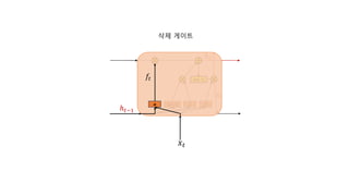
- 113. σ σ tan h tan h ℎ𝑡 𝑥𝑡 ℎ𝑡 삭제 게이트 ℎ𝑡−1 σ 𝑓𝑡
- 114. 셀 상태 𝑥𝑡 σ σ tan h tan h σ ℎ𝑡 ℎ𝑡 𝐶𝑡 𝐶𝑡−1 𝑓𝑡 𝑖𝑡 𝑔𝑡
- 115. 출력 게이트와 은닉 상태 σ tan h σ 𝑥𝑡 ℎ𝑡−1 𝐶𝑡−1 tan h ℎ𝑡 σ ℎ𝑡 𝑜𝑡
- 116. 태깅 작업 RNN의 다 대 다 문제 링크 : https://wikidocs.net/33805
- 117. 일 대 다(one-to-many) 다 대 일(many-to-one) 다 대 다(many-to-many) return_sequences = True 케라스에서 return_sequences=True를 하면 모든 time step에서 hidden state를 출력 시퀀스 레이블링 작업(ex) 태깅 작업)은 다 대 다 RNN으로 구현한다. 입력 시퀀스로부터 하나의 결론을 내는 작업(ex) 텍스트 분류)는 다 대 일 RNN으로 구현한다.
- 118. EU rejects GERMAN B-ORG O B-MISC 𝑥1 𝑦1 𝑥2 𝑦2 𝑥3 𝑦3 O x2 y2 𝑥4 𝑦4 call 단방향 RNN으로 태깅 작업을 할 경우
- 119. EU rejects GERMAN call B-ORG O B-MISC O 𝑦1 𝑦2 𝑦3 𝑦4 𝑥1 𝑥2 𝑥3 𝑥4 양방향 RNN으로 태깅 작업을 할 경우. 앞의 단어들도 참고하고 뒤의 단어들도 참고한다.
- 120. B-Org O 𝒘𝒐𝒓𝒅𝟏 𝒘𝒐𝒓𝒅𝟐 𝒘𝒐𝒓𝒅𝟑 𝒘𝒐𝒓𝒅𝟒 Activation Dense Activation Dense Activation Dense Activation Dense 0.7 0.12 0.08 0.04 0.06 I-Org B-Per I-Per embedding embedding embedding embedding 0.02 0.6 0.12 0.08 0.18 0.02 0.01 0.78 0.05 0.14 0.01 0.02 0.06 0.9 0.01 B-Per I-Per B-Org I-Org 양방향 RNN 개체명 인식 모델! 성능이 꽤 좋다. 그런데 아직도 개선할 것은 남아있다.
- 121. B-Org O 0.04 0.12 0.08 0.7 0.06 I-Org B-Per I-Per embedding embedding embedding embedding 0.02 0.6 0.12 0.08 0.18 0.02 0.01 0.14 0.05 0.78 0.01 0.02 0.06 0.9 0.01 I-Org I-Per O I-Org 양방향 RNN이 BIO 규칙을 제대로 반영하지 못 할 경우가 있다. 양방향 RNN은 이전 ‘레이블‘ 자체를 다음 ‘레이블'을 결정하는 일에 직접적으로 반영하지는 못 한다. 이전 ‘단어’를 참고는 하지만 예를 들어 I-Per을 결정할 때 앞에 I-Org라는 레이블이 등장했다는 사실에 대한 정보가 충분히 반영되지 못 한다. Activation Dense Activation Dense Activation Dense Activation Dense 𝒘𝒐𝒓𝒅𝟏 𝒘𝒐𝒓𝒅𝟐 𝒘𝒐𝒓𝒅𝟑 𝒘𝒐𝒓𝒅𝟒
- 122. B-Org O 0.7 0.12 0.08 0.04 0.06 I-Org B-Per I-Per embedding embedding embedding embedding 0.02 0.6 0.12 0.08 0.18 0.02 0.01 0.78 0.05 0.14 0.01 0.02 0.9 0.06 0.01 CRF 층을 추가하면 레이블간의 의존성을 고려하므로 B-I-O 패턴이라는 제약사항을 직접적으로 학습할 수 있다. CRF 𝒘𝒐𝒓𝒅𝟏 𝒘𝒐𝒓𝒅𝟐 𝒘𝒐𝒓𝒅𝟑 𝒘𝒐𝒓𝒅𝟒 Activation Dense Activation Dense Activation Dense Activation Dense B-Per I-Per I-Org I-Org B-Per O B-Org I-Per I-Per B-Org I-Org …… I-Per 예측 0.1 0.7 0.05 … CRF layer를 추가!
- 123. 링크 : https://wikidocs.net/33930 참고 : https://jalammar.github.io/illustrated-bert/
- 124. Broadway play produced by embedding embedding embedding embedding softmax 0.1 0.05 … 0.7 0.1 cat it … him unity Dense ELMo는 사전 훈련된 언어 모델을 사용
- 125. Broadway play produced embedding embedding embedding embedding embedding embedding 순방향 언어 모델 (Forward Language Model) 역방향 언어 모델 (Backward Language Model) Broadway play produced ELMo는 사전 훈련된 양방향 언어 모델을 사용 (기존의 BiLSTM하고는 다른데, ELMo에서는 양방향으로 분리해서 훈련하는 것에 가깝다.) 여기서는 순방향 언어 모델의 RNN 셀을 초록색, 역방향 언어 모델의 RNN 셀들을 초록색으로 표현하겠다.
- 126. embedding embedding embedding embedding embedding embedding 순방향 언어 모델 (Forward Language Model) 역방향 언어 모델 (Backward Language Model) Broadway play produced Broadway play produced Residual connection을 표현
- 127. embedding embedding embedding embedding embedding embedding 순방향 언어 모델 (Forward Language Model) 역방향 언어 모델 (Backward Language Model) Broadway play produced Broadway play produced
- 128. × s1 × s2 × s3 × s1 × s2 × s3 + + = γ × = ELMo 표현 연산 과정 1) 각 층의 출력값을 연결(concatenate)한다. 2) 각 층의 출력값 별로 가중치를 준다. 이 가중치를 여기서는 s1, s2, s3라고 합시다. 3) 각 층의 출력값을 모두 더한다. 2)번과 3)번의 단계를 요약하여 가중합(Weighted Sum)을 한다고 할 수 있습니다. 4) 벡터의 크기를 결정하는 스칼라 매개변수를 곱한다. 이 스칼라 매개변수를 여기서는 γ이라고 합시다.
- 129. ELMo 표현을 NLP 태스크에서 사용하는 방법의 예제 ELMo representation NLP Tasks Corpus biLMs Embedding vector embedding
- 131. je suis étudiant 기계 번역기 (SEQUENCE TO SEQUENCE) 인코더 (Encoder) 디코더 (Decoder) SEQ2SEQ 모델 CONTEXT I am a student je suis étudiant I am a student 기계 번역은 대표적으로 seq2seq 구조를 가지는 예이다. 여기서는 인코더의 RNN 셀들을 주황색 디코더의 RNN 셀들을 초록색으로 표현하겠다.
- 132. CONTEXT LSTM LSTM LSTM LSTM 디코더(Decoder) 0.15 0.21 -0.11 0.91 CONTEXT I am a student je suis étudiant <eos> <sos> je suis étudiant LSTM LSTM LSTM LSTM 인코더(Encoder) 0.157 -0.25 0.478 -0.78 I 0.78 0.29 -0.96 0.52 am 0.75 -0.81 0.96 0.12 a 0.88 0.17 -0.29 0.48 student 위의 벡터들은 임베딩 벡터들을 나타낸다. 위 벡터는 컨텍스트 벡터를 나타낸다.
- 133. CONTEXT LSTM LSTM LSTM LSTM 디코더(Decoder) 0.15 0.21 -0.11 0.91 CONTEXT I am a student je suis étudiant <eos> <sos> je suis étudiant 0.15 0.21 -0.11 0.91 I 0.15 0.21 -0.11 0.91 am 0.15 0.21 -0.11 0.91 a 0.15 0.21 -0.11 0.91 student embedding layer LSTM LSTM LSTM LSTM 인코더(Encoder) embedding embedding embedding embedding embedding embedding embedding embedding 아래의 벡터는 인코더의 hidden state를 의미한다.
- 134. 현재 time step t에서의 입력 벡터 현재 time step t에서의 은닉 상태 time step t-1에서의 은닉 상태 time step t에서의 은닉 상태 RNN 셀의 입, 출력을 보여준다. LSTM 셀으로 생각할 경우에는 cell state는 그림에서 생략되었다고 봐야한다.
- 135. LSTM LSTM LSTM LSTM 디코더(Decoder) je suis étudiant <eos> <sos> je suis étudiant embedding embedding embedding embedding softmax softmax softmax softmax Dense Dense Dense Dense 디코더는 기본적으로 RNN 언어모델이다. 이전 time step의 출력을 다음 time step의 입력으로 사용하는 Generation 모델이기 때문이다. Decoder RNN: A language model that generates the target sentence conditioned with the encoding created by the encoder.
- 136. LSTM LSTM LSTM LSTM 디코더(Decoder) <sos> je suis étudiant embedding embedding embedding embedding CONTEXT I am a student LSTM LSTM LSTM LSTM 인코더(Encoder) embedding embedding embedding embedding je suis étudiant <eos> softmax softmax softmax softmax Dense Dense Dense Dense 완전체 그림
- 137. seq2seq+attention 링크 : https://wikidocs.net/22893 참고 : https://web.stanford.edu/class/cs224n/assi gnments/a4.pdf
- 138. Query Attention Value Key1 Key2 Key3 Value1 Value2 Value3 Source 어텐션을 함수로 표현한 경우를 보여준다.
- 139. étudiant softmax LSTM LSTM LSTM <sos> je suis embedding embedding embedding I am a student LSTM LSTM LSTM LSTM embedding embedding embedding embedding softmax Dense seq2seq + attention의 완전체 그림
- 140. LSTM LSTM LSTM <sos> je suis embedding embedding embedding I am a student LSTM LSTM LSTM LSTM embedding embedding embedding embedding dot product ℎ1 ℎ2 ℎ3 ℎ4 𝑠𝑡−1 𝑇 Attention Score 𝑒𝑡 = [𝑠𝑡−1 𝑇 ℎ1, . . . , 𝑠𝑡−1 𝑇 ℎ𝑁] score(𝑠𝑡−1, ℎ𝑖) = 𝑠𝑡−1 𝑇 ℎ𝑖 1. 우선 어텐션 스코어를 구한다.
- 141. ℎ𝑖 𝑠𝑡−1 𝑇 × 이름 어텐션 스코어 함수 1. 어텐션 스코어를 구하는 방법을 여기서는 dot product(내적)을 사용하였지만 사실 어텐션 스코어 함수를 무엇을 사용하는지에 따라 다르다.
- 142. LSTM LSTM LSTM <sos> je suis embedding embedding embedding I am a student LSTM LSTM LSTM LSTM embedding embedding embedding embedding softmax Attention Distribution 2. 어텐션 분포를 구한다. 𝑒𝑡 = 𝑠𝑡−1 𝑇 ℎ1, . . . , 𝑠𝑡−1 𝑇 ℎ𝑁 𝑒𝑡에 소프트맥스 함수를 사용한다.
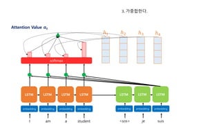
- 143. LSTM LSTM LSTM <sos> je suis embedding embedding embedding I am a student LSTM LSTM LSTM LSTM embedding embedding embedding embedding softmax Attention Value 𝒂𝒕 ℎ1 ℎ2 ℎ3 ℎ4 3. 가중합한다.
- 144. LSTM LSTM LSTM <sos> je suis embedding embedding embedding softmax concatenate Attention Value 𝒂𝒕 𝒔𝒕−𝟏 𝑣𝑡 4. 연결한다.
- 145. simple seq2seq 케라스에서는 RepeatVector를 사용하여 아주 간단한 seq2seq를 빠르게 구현할 수 있다. 링크 : https://wikidocs.net/43646
- 146. LSTM LSTM LSTM LSTM 디코더(Decoder) 𝑥1 LSTM LSTM LSTM LSTM 인코더(Encoder) ? 𝑥2 𝑥𝑛−1 𝑥𝑛 … … … 𝑥1 𝑥2 𝑥𝑚−1 𝑥𝑚 …
- 147. 𝑥1 LSTM LSTM LSTM 𝑥2 𝑥𝑛−1 𝑥𝑛 … … ℎ𝑛 𝑛 time-steps LSTM last hidden state
- 148. LSTM 디코더(Decoder) 𝑥1 LSTM LSTM LSTM LSTM 인코더(Encoder) 𝑥2 𝑥𝑛−1 𝑥𝑛 … … … 𝑥1 𝑥2 𝑥𝑚−1 𝑥𝑚 … model = Sequential() model.add(LSTM(..., input_shape=(...))) model.add(RepeatVector(...)) model.add(LSTM(..., return_sequences=True)) model.add(TimeDistributed(Dense(...))) ℎ𝑛 last hidden state LSTM RepeatVector LSTM LSTM 놀랍게도 이 구조가 전부이다!
- 149. Char CNN
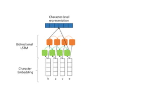
- 150. <pad> h a v e <pad> <pad> <pad> Character Embedding 1D Convolution Max-pooling Character-level representation
- 151. h a v e Padding Padding Character Embedding 1D Convolution Max-pooling concatenate Filter Size = 3 Character-level representation
- 152. Char RNN
- 154. 트랜스포머 링크 : https://wikidocs.net/31379 참고 : http://jalammar.github.io/illustrated- transformer/
- 155. 트랜스포머(Transformer) I am a student je suis étudiant 인코더들 (Encoders) 디코더들 (Decoders) 트랜스포머 모델 I am a student je suis étudiant 인코더 #1 트랜스포머 모델 I am a student je suis étudiant 인코더 #2 인코더 #3 인코더 #4 인코더 #5 인코더 #6 디코더 #1 디코더 #2 디코더 #3 디코더 #4 디코더 #5 디코더 #6
- 156. I am a student embedding embedding embedding embedding je suis étudiant <eos> <sos> je suis étudiant embedding embedding embedding embedding Encoders Decoders Positional Encoding I am a student embedding embedding embedding embedding Positional Encoding je suis étudiant <eos> <sos> je suis étudiant embedding embedding embedding embedding Encoders Decoders 포지셔널 인코딩이란?
- 157. I am a student embedding vector : positional encoding : + + + + I am a student + 임베딩 벡터에 값을 더해준다. 그런데 사실 이는 행렬 연산으로도 이해 가능하다.
- 159. 인코더(Encoder) embedding Positional Encoding Multi-head Self-Attention Position-wise FFNN Add & Norm Add & Norm num_layer × 인코더(Encoder) Self-Attention FFNN Add & Normalize Add & Normalize 인코더(Encoder) FFNN Self-Attention 어느게 더 표현하기 좋을까 여러 개 그려봤다.
- 160. 인코더(Encoder) FFNN Multi-head Self-Attention I am a student embedding embedding embedding embedding Positional Encoding I am a student LSTM LSTM LSTM LSTM embedding embedding embedding embedding Attention Distribution softmax LSTM 관점에서 생각해보는 셀프 어텐션
- 161. student 𝑊𝑄 𝑊𝐾 𝑊𝑉 × × × = = = 𝑄𝑠𝑡𝑢𝑑𝑒𝑛𝑡 𝐾𝑠𝑡𝑢𝑑𝑒𝑛𝑡 𝑉𝑠𝑡𝑢𝑑𝑒𝑛𝑡 인코더의 셀프 어텐션은 가중치 행렬의 곱으로부터 얻은 Q, K, V 벡터로 수행한다.
- 162. 128 128 / 𝑑𝑘= 16 32 32 / 𝑑𝑘= 4 32 32 / 𝑑𝑘= 4 = 𝐾𝑠𝑡𝑢𝑑𝑒𝑛𝑡 𝑇 𝐾𝐼 𝑇 𝐾𝑎𝑚 𝑇 𝐾𝑎 𝑇 𝑄𝐼 × × × × = = = Scaled dot product Attention : 𝒔𝒄𝒐𝒓𝒆 𝒇𝒖𝒏𝒄𝒕𝒊𝒐𝒏 𝒒, 𝒌 = 𝒒⋅𝒌/ 𝒏 128 128 / 𝑑𝑘= 16 Attention Score
- 163. 128 128 / 𝑑𝑘= 16 0.4 0.4 32 32 / 𝑑𝑘= 4 0.1 0.1 32 32 / 𝑑𝑘= 4 0.1 0.1 = = 𝐾𝑠𝑡𝑢𝑑𝑒𝑛𝑡 𝑇 𝐾𝐼 𝑇 𝐾𝑎𝑚 𝑇 𝐾𝑎 𝑇 𝑄𝐼 × × × × = = = 𝑉𝑠𝑡𝑢𝑑𝑒𝑛𝑡 𝑉 𝑎 𝑉 𝑎𝑚 𝑉𝐼 softmax × 128 128 / 𝑑𝑘= 16 0.4 0.4 × × × Attention Distribution + + + Attention Value
- 164. 𝑊𝑄 𝑊𝐾 𝑊𝑉 × × × = = = 𝑉𝑠𝑡𝑢𝑑𝑒𝑛𝑡 I am a student 𝑄 𝐾 𝐼 𝑎𝑚 𝑎 𝑠𝑡𝑢𝑑𝑒𝑛𝑡 𝐼 𝑎𝑚 𝑎 𝑠𝑡𝑢𝑑𝑒𝑛𝑡 𝐼 𝑎𝑚 𝑎 𝑠𝑡𝑢𝑑𝑒𝑛𝑡 행렬 연산을 이용하면 병렬로 수행할 수 있다.
- 165. 𝑎 × = = 𝐼 𝑎𝑚 𝑎 𝑠𝑡𝑢𝑑𝑒𝑛𝑡 𝑲𝑻 𝑸 𝐼 𝑎𝑚 𝑎 𝑠𝑡𝑢𝑑𝑒𝑛𝑡 𝐼 𝑎𝑚 𝑠𝑡𝑢𝑑𝑒𝑛𝑡 𝐼 𝑎𝑚 𝑎 𝑠𝑡𝑢𝑑𝑒𝑛𝑡 Attention Score Matrix
- 166. 𝑲𝑻 softmax ( ) × = 𝑸 𝑑𝑘 𝑉𝑠𝑡𝑢𝑑𝑒𝑛𝑡 × = Attention Value Matrix 𝒂
- 167. 𝑊 0 𝑄 𝑊0 𝐾 𝑊0 𝑉 I am a student Attention #0 𝒂𝟎 𝑊 1 𝑄 𝑊1 𝐾 𝑊1 𝑉 Attention #1 𝒂𝟏 num_heads만큼 수행 𝒂𝒏𝒖𝒎_𝒉𝒆𝒂𝒅𝒔 Attention #num_heads …
- 168. 𝒂𝟎 𝒂𝟏 𝒂𝟐 concatenate 𝒂𝟒 𝒂𝟓 𝒂𝟔 𝒂𝟕 𝒂𝟖 𝑊𝑂 𝑑𝑚𝑜𝑑𝑒𝑙 = 𝑑𝑣 × num_heads 𝑑𝑚𝑜𝑑𝑒𝑙 = 𝑑𝑣 × num_heads 𝑑𝑚𝑜𝑑𝑒𝑙
- 169. 𝑾𝑶 𝑑𝑣 × num_heads 𝑑𝑚𝑜𝑑𝑒𝑙 𝑑𝑚𝑜𝑑𝑒𝑙 = 𝑑𝑣 × num_heads × concatenated matrix seq_len = Multi-head attention matrix
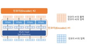
- 170. Multi-head Self-Attention 인코더(Encoder) #1 FFNN FFNN FFNN FFNN 인코더 #1의 출력 인코더 #2의 입력 인코더 #1의 입력 인코더(Encoder) #2
- 171. Multi-head Self-Attention 인코더(Encoder) #1 FFNN FFNN FFNN FFNN Add & Norm Add & Norm
- 172. 𝑥 𝐹1 = 𝑥𝑊1 + 𝑏1 활성화 함수 ∶ 𝑅𝑒𝐿𝑈 𝐹2 = max(0, 𝐹1) 𝐹3 = 𝐹2𝑊2 + 𝑏2 Position-wise FFNN 𝑥 𝐹(𝑥) + 𝐻 𝑥 = 𝑥 + 𝐹(𝑥) Residual Connection
- 173. 인코더(Encoder) #1 FFNN FFNN FFNN FFNN Add & Norm Add & Norm Multi-head Self-Attention 8. 잔차 연결(Residual connection)과 층 정규화(Layer Normalization)
- 174. Multi-head Self-Attention #1 FFNN #1 FFNN #1 FFNN #1 FFNN #1 Multi-head Self-Attention #2 FFNN #2 FFNN #2 FFNN #2 FFNN #2 I am a student 인코더(Encoder) #1 인코더(Encoder) #2
- 175. Decoder Masked Input Positional Encoding I am a student embedding embedding embedding embedding Positional Encoding je suis étudiant <eos> <sos> je suis étudiant embedding embedding embedding embedding Encoders Decoders <sos> je suis étudiant <sos> je suis étudiant <sos> je suis étudiant
- 176. embedding Positional Encoding Multi-head Self-Attention Add & Norm num_layers × embedding Positional Encoding Multi-head Self-Attention Add & Norm softmax × num_layers Multi-head Self-Attention Add & Norm Add & Norm Position-wise FFNN Dense Add & Norm Position-wise FFNN
- 177. Pre-training
- 178. Semi-Supervised Sequence Learning, Google, 2015 <SOS> I am I am a student x2 y2 a LSTM LSTM LSTM LSTM I Iove you positive x2 y2 3000 LSTM LSTM LSTM LSTM LSTM 언어 모델을 사전 훈련 분류 문제에 파인 튜닝
- 179. ELMo: Deep Contextual Word Embedding, AI2 & University of Washington, 2017 <SOS> I am I am a student x2 y2 a LSTM LSTM LSTM LSTM <SOS> I am I am a student x2 y2 a LSTM LSTM LSTM LSTM
- 180. ELMo: Deep Contextual Word Embedding, AI2 & University of Washington, 2017 NLP Tasks biLMs <SOS> I am I am a student x2 y2 a LSTM LSTM LSTM LSTM <SOS> I am I am a student x2 y2 a LSTM LSTM LSTM LSTM 순방향 언어 모델과 역방향 언어 모델을 각각 훈련 사전 훈련된 임베딩에 사용
- 181. Improving Language Understanding by Generative Pre-training, OpenAI, 2018 <SOS> I am I am a student x2 y2 a Trm Trm Trm I Iove you positive x2 y2 3000 Trm Trm Trm Trm Deep(12-layer) Trm 언어 모델을 사전 훈련 분류 문제에 파인 튜닝 Trm
- 182. 단방향 언어모델 양방향 언어모델 순차적으로 단어를 생성한다. 단어들이 자기 자신을 본다. <SOS> I am a I am a student <SOS> I am a I am a student
- 183. BERT
- 184. BERT Masked Language Model 33억 단어에 대해서 4일간 학습시킨 언어 모델 BooksCorpus 스팸 메일 분류기 BERT softmax FFNN
- 185. BERT-Base Transformer Encoder Transformer Encoder Transformer Encoder … Transformer Encoder Transformer Encoder 12개 layer BERT-Large Transformer Encoder Transformer Encoder Transformer Encoder … Transformer Encoder Transformer Encoder 24개 layer
- 186. BERT(12-layers) Dense [CLS] I love you embedding 긍정 사람 BERT(12-layers) [CLS] When Sebastian Thrun embedding Dense Dense Dense X 사람 감성 분류 개체명 인식
- 187. BERT(12-layers) Dense [CLS] I love you embedding Positive [SEP]
- 188. X BERT(12-layers) [CLS] Mike joined Aiimi embedding Dense Dense Dense Person Organization [SEP] BERT(12-layers)
- 189. BERT(12-layers) [CLS] my dog is cute [SEP] he likes play ##ing [SEP] Dense True
- 190. BERT(12-layers) [CLS] Token1 [SEP] [SEP] Label Token2 Token3 Token4 Token5 Token6 Token7 Token8 Dense Dense Dense Dense
- 191. BERT(12-layers) [CLS] I love love 입력 임베딩 출력 임베딩 [CLS] I you you
- 192. BERT(12-layers) [CLS] I love you love BERT(12-layers) [CLS] I love you [CLS] 입력 임베딩 출력 임베딩
- 193. [CLS] I love you BERT Layer #1
- 194. [CLS] I love you BERT Layer #2 … BERT Layer #12 Multi-head Self-Attention FFNN FFNN FFNN FFNN Add & Norm Add & Norm
- 195. BERT(12-layers) [CLS] I love you 0 1 2 3 + + + + Word Embedding Position Embedding
- 196. BERT(12-layers) Dense [CLS] I love you embedding 긍정 BERT(12-layers) Dense [CLS] I love you embedding 긍정
- 197. BERT(12-layers) [CLS] my dog is 0 1 2 3 + + + + WordPiece Position cute 4 + [SEP] he likes play 5 6 7 8 + + + + ##ing 9 + [SEP] 10 + 0 0 0 0 + + + + 0 + 0 1 1 1 + + + + 1 + 1 + Segment Dense
- 198. cat BERT(12-layers) [CLS] my [MASK] is cute [SEP] he likes play ##ing [SEP] MLM Classifier
- 199. MLM Classifier BERT(12-layers) [CLS] my [MASK] is cute [SEP] king likes play ##ing [SEP] MLM Classifier MLM Classifier
- 200. MLM Classifier BERT(12-layers) [CLS] my [MASK] is cute [SEP] king likes play ##ing [SEP] MLM Classifier MLM Classifier NSP Classifier
- 201. BERT(12-layers) [CLS] my dog is cute [SEP] [PAD] [PAD] [PAD] [PAD] [PAD] Dense 1 1 1 1 1 1 0 0 0 0 0
- 202. 85.0% 12.0% 1.5% 1.5% 전체 단어 미사용 [MASK]로 변경 후 예측 랜덤으로 변경 후 예측 미변경 후 예측
- 203. Sentence bert
- 204. BERT(12-layers) [CLS] I love love [CLS] I you you pooling 해당 문장의 표현 벡터
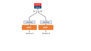
- 205. BERT Sentence A pooling u BERT Sentence B pooling v (u; v; |u-v|)
- 206. BERT Sentence A pooling u BERT Sentence B pooling v (u; v; |u-v|) softmax Dense
- 207. BERT Sentence A pooling u BERT Sentence B pooling v 코사인 유사도(u, v)