


![1.1. SOURCE OF DATA BLOCKS 21
Here, % sign is used to represent modulo in numerical programming. Modulo counter
block simulation is given below
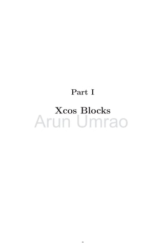
Clock c
CScope
Counter
Modulo 10
Modulo Counter
Figure 1.31: In this configuration, a clock is used to refresh the single scope for showing
the counter modulo 10.
1.1.13 Ramp
Ramp block provide output values according to the relation
y = mt + c
Where y is value provided by ramp at any instant of time t. m, t c are ramp parameters.
m is slope of ramp that determines how fast the output values varies. t is time function
that increases continuously from its initial value. c is initial value of ramp output. Ramp
has only one output port. Derivating to ramp relation
m =
dy
dt
The right side of above relation represent to velocity parameter, therefore, ramp function
also represents to velocity function. The symbol of ramp function is
Figure 1.32: Ramp block (Ramp)
1.1.14 Random Generator
Random generator block generates random values within the two given ranges. The
random value generated by this block is received when clock triggers the block. It has
one control port and one output port. Mathematically
r = R(t)
where, r is sampled random value and R(t) is random value generated by the random
block at time t. The random value r has range a ≤ r ≤ b, i.e. within domain of [a, b].
Arun
is value provided by ramp at any instant of time
is value provided by ramp at any instant of time
is slope of ramp that determines how fast the output values varies.
is slope of ramp that determines how fast the output values varies.
Umrao
mt +
+ c
is value provided by ramp at any instant of time
is value provided by ramp at any instant of time t.
. m,
, t
t
c
c are ramp parameters.
are ramp parameters.
is slope of ramp that determines how fast the output values varies.
is slope of ramp that determines how fast the output values varies. t
t](https://image.slidesharecdn.com/xcosscilabblockdescriptionswithsuitableexamples-211010151413/85/Notes-and-Description-for-Xcos-Scilab-Block-Simulation-with-Suitable-Examples-by-Arun-Umrao-21-320.jpg)

![1.1. SOURCE OF DATA BLOCKS 23
then ith
element of the read record is assumed to be the date of the output event,
i.e. this record is treated as value of t-axis (time variable).
2. Outputs record selection : It is a vector of positive integers like [1, 2, 5]. If read data
is like a vector [k1, k2, . . . kn] then kth
i elements of the read records, i.e. the vector
made of elements [k1, k2, k5] is given in output.
3. Input file name is a file name or path file name. Its value is string of characters.
4. Buffer size : It is similar to the number of bytes read by fread function of C language.
To improve efficiency of input read, file is only done after each Buffer size call to
the block.
For example, consider a data file myfle.txt with following data except label row
Arun Umrao](https://image.slidesharecdn.com/xcosscilabblockdescriptionswithsuitableexamples-211010151413/85/Notes-and-Description-for-Xcos-Scilab-Block-Simulation-with-Suitable-Examples-by-Arun-Umrao-23-320.jpg)
![24 Blocks Pallets
C1 C2 C3
01 0.100 -0.100
02 0.199 -0.199
03 0.296 -0.296
04 0.389 -0.389
05 0.479 -0.479
06 0.565 -0.565
07 0.644 -0.644
08 0.717 -0.717
09 0.783 -0.783
10 0.841 -0.841
11 0.891 -0.891
12 0.932 -0.932
13 0.964 -0.964
14 0.985 -0.985
15 0.997 -0.997
16 1.000 -1.000
17 0.992 -0.992
18 0.974 -0.974
19 0.946 -0.946
20 0.909 -0.909
21 0.863 -0.863
22 0.808 -0.808
23 0.746 -0.746
24 0.675 -0.675
25 0.598 -0.598
26 0.516 -0.516
27 0.427 -0.427
28 0.335 -0.335
29 0.239 -0.239
30 0.141 -0.141
31 0.042 -0.042
32 -0.058 0.058
Each row has data record for different entity. Hence the unique data vector for each
row is [k1, k2, k3]. If time record selection is 1, then first column will be used at t values,
i.e. time event values. If this option has value 2, then second column is used at time even
values. Note that, time value is always 0 and continuous increasing, hence block stops
reading of data when either time becomes negative or time starts decreasing. So, time
Arun
16 1.000 -1.000
17
1
18 0.974 -0.974
8 0.974 -0.974
Umrao
6 1.000 -1.000
6 1.000 -1.000
0. -0.992
8 0.974 -0.974
8 0.974 -0.974](https://image.slidesharecdn.com/xcosscilabblockdescriptionswithsuitableexamples-211010151413/85/Notes-and-Description-for-Xcos-Scilab-Block-Simulation-with-Suitable-Examples-by-Arun-Umrao-24-320.jpg)
![1.1. SOURCE OF DATA BLOCKS 25
column should be positive, greater than zero and continuous increasing. There are three
output records. If output record selection has value 1 then only data of first column is
sent as output of this block. If the output record selection has value [123] then values in
first, second and third columns will be sent as output of this block.
Clock c
CScope
Read data
from input file
RFILE f
The time record selection is 1 and output record selection is [2, 3]. The output will be
as
−1
0
1
0 3 6 9 12 15 18 21 24 27 30
y
t
If the time record selection is 2 and output record selection is [2, 3], then time for data
read shall be from t = 0 to t = 1 seconds. After than time starts decreasing hence reading
block will stop reading of data from input data file. And the output will be as
−1
0
1
0 3 6 9 12 15 18 21 24 27 30
y
t
If the time record selection is 3 and output record selection is [2, 3], then time for data
read shall be from t = 0 to t = 0 seconds as time value is negative. There will be no
output. Similarly, if time record selection option value is empty, then there is null time,
hence no output.
Arun
Arun
Arun Umrao
Umrao
Umrao](https://image.slidesharecdn.com/xcosscilabblockdescriptionswithsuitableexamples-211010151413/85/Notes-and-Description-for-Xcos-Scilab-Block-Simulation-with-Suitable-Examples-by-Arun-Umrao-25-320.jpg)

![1.1. SOURCE OF DATA BLOCKS 27
Read from
‘C’ binary file
Figure 1.35: Read from ‘C’ binary file (READC f).
This block uses configure options.
1. Time Record Selection : It is either an empty matrix or an strictly positive integer
greater than zero (scalar). If it is empty, there is no output event port exists. If
an integer value, ‘i’, is given, then ith
element of the read record is assumed to be
the time event value of the output event port, i.e. this record is treated as value of
t-axis (time variable). If this option has value greater than zero, then one command
port is created in this block and ith
will be used as time axis value and also may be
used to control scope viewers.
2. Outputs Record Selection : It is a vector of positive integers like [1, 2, 5]. If read
data is like a vector [k1, k2, . . . kn] then kth
i elements of the read records, i.e. the
vector made of elements [k1, k2, k5] is given in output.
3. Input File Name : It is a file name or path file name. Its value is string of characters.
4. Input Format : A character string defining the data format to use. Strings “l”, “i”,
“s”, “ul”, “ui”, “us”, “d”, “f”, “c”, “uc” are used respectively to write int32, int16,
int8, uint32, uint16, uint8, double, float, char or unsigned char data type. This
value must be same as the value of Output Format option of WRITEC f block.
5. Record Size : This specify the number of columns to be read from C binary file.
This should be same as the input size option of WRITEC f block. If this value is
2 and data being read from C binary file is integer type, then 8 bytes data shall be
read for one record. It is vector of size one.
6. Buffer Size : It is similar to the number of bytes read by fread function of C language.
7. Initial Record Index : This fixes the first record of the file to use. For example, if
record of each entity is arranged in one line and this option is set four, then file will
be read from the fourth line in place of first line.
8. Swap Mode : If Swap mode=1 then file is supposed to be coded in “little endian
IEEE format” and data are swapped if necessary to match the IEEE format of the
processor. If Swap mode=0 then automatic bytes swap is disabled.
A simple block arrangement is shown below:
Arun
4. Input Format : A character string defining the data format to use. Strings “l”, “i”,
4. Input Format : A character string defining the data format to use. Strings “l”, “i”,
“s”, “ul”, “ui”, “us”, “d”, “f”, “c”, “uc” are used respectively to write int32, int16,
“s”, “ul”, “ui”, “us”, “d”, “f”, “c”, “uc” are used respectively to write int32, int16,
int8, uint32, uint16, uint8, double, float, char or unsigned char data type. This
int8, uint32, uint16, uint8, double, float, char or unsigned char data type. This
Umrao
4. Input Format : A character string defining the data format to use. Strings “l”, “i”,
4. Input Format : A character string defining the data format to use. Strings “l”, “i”,
“s”, “ul”, “ui”, “us”, “d”, “f”, “c”, “uc” are used respectively to write int32, int16,
“s”, “ul”, “ui”, “us”, “d”, “f”, “c”, “uc” are used respectively to write int32, int16,
int8, uint32, uint16, uint8, double, float, char or unsigned char data type. This
int8, uint32, uint16, uint8, double, float, char or unsigned char data type. This](https://image.slidesharecdn.com/xcosscilabblockdescriptionswithsuitableexamples-211010151413/85/Notes-and-Description-for-Xcos-Scilab-Block-Simulation-with-Suitable-Examples-by-Arun-Umrao-27-320.jpg)


![1.2. SINK OF DATA BLOCKS 31
1.2.3 Floating Point Scope
Floating point scope, shows output of floating points ranges between zero to one. It has
one control port. The output viewed in this scope is
y = (float)x
Figure 1.40: Floating Point Scope (CFSCOPE)
Following parameters of the block can be set as and when required.
Color Set the number for color of output graph.
Output Window Number Output windows are assigned an identification numbers for
processing of data. By default it is ‘-1’. It means the window number will automatically
assigned an ID. Apart from it, user defined ID can also be assigned to the window.
Output Window Position Position of window tell the window that where it will posi-
tioned after opening. By default it is positioned in center of screen. The xy-coordinates
of window position are assigned like [x; y]. The coordinates are calculated from the top
left corner of the screen of computer system.
Output Window Sizes It determines the size of output window. The coordinates are
syntax as [x; y].
Ymin It is the minimum value of the output to be displayed in the output window.
Ymin is used to set the lower scale point of the y-axis in output display.
YMax It is the maximum value of the output to be displayed in the output window.
Ymax is used to set the upper scale point of the y-axis in output display.
Refresh Period It is the maximum range of independent variable to be displayed in
the output window.
Buffer Size The size of output values to be stored in the memory. The drawing is
only done after each Buffer size call to the block.
1.2.4 XY Animated Viewer
XY animated viewer visualized the second input with respect first input as a function of
first input at instant simulated time. Mathematically
y = f(x)
The output plot is two dimensional. It has two input ports and one control port. One of
the two input ports is for variable and second is for function of variable.
Arun
Output Window Position
Output Window Position Position of window tell the window that where it will posi-
Position of window tell the window that where it will posi-
ioned after opening. By default it is positioned in center of screen. The xy-coordinates
ioned after opening. By default it is positioned in center of screen. The xy-coordinates
of window position are assigned like [
of window position are assigned like [ Umrao
Position of window tell the window that where it will posi-
Position of window tell the window that where it will posi-
ioned after opening. By default it is positioned in center of screen. The xy-coordinates
ioned after opening. By default it is positioned in center of screen. The xy-coordinates
y]. The coordinates are calculated from the top
]. The coordinates are calculated from the top](https://image.slidesharecdn.com/xcosscilabblockdescriptionswithsuitableexamples-211010151413/85/Notes-and-Description-for-Xcos-Scilab-Block-Simulation-with-Suitable-Examples-by-Arun-Umrao-31-320.jpg)


![1.2. SINK OF DATA BLOCKS 37
0.4285714
0.5714286
0.7142857
0.8571429
1.
Let the matrix elements are arranged in the xy-plane taking x-axis as rows and y-axis as
columns. The experimental matrix is
1 -- M=[0 1 2; 2 3 4; 4 5 6;6 7 8]
M=
0. 1. 2.
2. 3. 4.
4. 5. 6.
6. 7. 8.
Now, the minimum matrix value (say 0) is set to gray color level 0 and maximum matrix
value (say 8) is set to gray color level 1. The intermediate distinct matrix elements are
assigned proposed gray color code from equally distributed gray colormap values ranging
from 0 to 1 as shown in the below table.
Matrix Element Proposed Gray Code
0 0.000
1 0.125
2 0.250
3 0.375
4 0.500
5 0.625
6 0.750
7 0.875
8 1.000
As there are 8 colormap levels and 9 distinct matrix elements, hence the proposed
gray color codes are rounded to near gray colormap values of actual gray colormap. Thus
the actual table will be
Arun
Matrix Elemen
Umrao
Proposed Gray Code
0.000](https://image.slidesharecdn.com/xcosscilabblockdescriptionswithsuitableexamples-211010151413/85/Notes-and-Description-for-Xcos-Scilab-Block-Simulation-with-Suitable-Examples-by-Arun-Umrao-37-320.jpg)


![1.2. SINK OF DATA BLOCKS 47
1. Input Size : It is size of input column vector. A scalar that determines the how
many columns of data values are used to form a record. This description must
be read with the data output format description. Suppose, we have define integer
datatype data format and input size is 2 then total 8 bytes shall be used to write a
record of data in binary form. The data received at input port of WRITEC f block
must be of same size as defined in the Input Size option.
2. Output File Name : It is a file name or path file name where data would be written.
Its value is string of characters.
3. Output Format : A character string defining the data format to use. Strings “l”,
“i”, “s”, “ul”, “ui”, “us”, “d”, “f”, “c”, “uc” are used respectively to write int32,
int16, int8, uint32, uint16, uint8, double, float, char or unsigned char data type.
4. Buffer Size : It is similar to the number of bytes read by fread function of C language.
5. Swap Mode : If swap mode=1 then file is supposed to be coded in “little endian
IEEE format” and data are swapped if necessary to match the IEEE format of the
processor. If Swap mode=0 then automatic bytes swap is disabled.
Clock c
Write to C
GenSin f
The above block diagram is indicative purpose about the use of WRITEC f. The data
written by this block is in format as shown below:
rec[4]
20 4
byte[1] byte[2]
rec[5]
40 12
byte[1] byte[2]
rec[6]
60 20
byte[1] byte[2]
rec[7]
80 28
byte[1] byte[2]
wr
In this figure, we have explained that the character type data with size two is saved in
binary format. First byte is for one of the two data elements of a record and second byte
is for other of the two data elements of a record. The number of bytes required depends
on the type of data and size of data. A character data type requires one byte memory
space and if record size is two then two bytes are required to save a record. If data type
is integer type and data size is two, then memory arrangement shall be like
rec[4]
0 0 20 4
byte[1] byte[2] byte[3] byte[4]
rec[5]
0 0 40 12
byte[1] byte[2] byte[3] byte[4]
rec[6]
0 0 60 20
byte[1] byte[2] byte[3] byte[4]
wr
Arun Umrao
Umrao
Umrao
Umrao
Umrao
Umrao
Umrao
Umrao
Umrao
Umrao
Umrao
Umrao
Umrao
Umrao
Umrao
Umrao
Umrao
Umrao
Umrao
Umrao
Umrao
Umrao
Umrao
Umrao
Umrao
Umrao
Umrao
Umrao
Umrao
Umrao
Umrao
Umrao
Umrao
Umrao
Umrao
Umrao
Umrao
Umrao
Umrao
Umrao
Umrao
Umrao
Umrao
Umrao
Umrao
Umrao
Umrao
Umrao
Umrao
Umrao
Umrao
Umrao
Umrao
Umrao
Umrao
Umrao
Umrao
Umrao
Umrao
Umrao
Umrao
Umrao
Umrao
Umrao
Umrao
Umrao
Umrao
Umrao
Umrao
Umrao
Umrao
Umrao
Umrao
Umrao
Umrao
Umrao
Umrao
Umrao
Umrao
Umrao
Umrao
Umrao
Umrao
Umrao
Umrao
Umrao
Umrao
Umrao
Umrao
Umrao
Umrao
Umrao
Umrao
Umrao
Umrao
Umrao
Umrao
Umrao
Umrao
Umrao
Umrao
Umrao
Umrao
Umrao
Umrao
Umrao
Umrao
Umrao
Umrao
Umrao
Umrao
Umrao
Umrao
Umrao
Umrao
Umrao
Umrao
Umrao
Umrao
Umrao
Umrao
Umrao
Umrao
Umrao
Umrao
Umrao
Umrao
Umrao
Umrao
Umrao
Umrao
Umrao
Umrao
Umrao
Umrao
Umrao
Umrao
Umrao
Umrao
Umrao
Umrao
Umrao
Umrao
Umrao
Umrao
Umrao
Umrao
Umrao
Umrao
Umrao
Umrao
Umrao
Umrao
Umrao
Umrao
Umrao
Umrao
Umrao
Umrao
Umrao
Umrao
Umrao
Umrao
Umrao
Umrao
Umrao
Umrao
Umrao
Umrao
Umrao
Umrao
Umrao
Umrao
Umrao
Umrao
Umrao
Umrao
Umrao
Umrao
Umrao
Umrao
Umrao
Umrao
Umrao
Umrao
Umrao
Umrao
Umrao
Umrao
Umrao
Umrao
Umrao
Umrao
Umrao
Umrao
Umrao
Umrao
Umrao
Umrao
Umrao
Umrao
Umrao
Umrao
Umrao
Umrao
Umrao
Umrao
Umrao
Umrao
Umrao
Umrao
Umrao
Umrao
Umrao
Umrao
Umrao
Umrao
Umrao
Umrao
Umrao
Umrao
Umrao
Umrao
Umrao
Umrao
Umrao
Umrao
Umrao
Umrao
Umrao
Umrao
Umrao
Umrao
Umrao
Umrao
Umrao
Umrao
Umrao
Umrao
Umrao
Umrao
Umrao
Umrao
Umrao
Umrao
Umrao
Umrao
Umrao
Umrao
Umrao
Umrao
Umrao
Umrao
Umrao
Umrao
Umrao
Umrao
Umrao
Umrao
Umrao
Umrao
Umrao
Umrao
Umrao
Umrao
Umrao
Umrao
Umrao
Umrao
Umrao
Umrao
Umrao
Umrao
Umrao
Umrao
Umrao
Umrao
Umrao
Umrao
Umrao
Umrao
Umrao
Umrao
Umrao
Umrao
Umrao
Umrao
Umrao
Umrao
Umrao
Umrao
Umrao
Umrao
Umrao
Umrao
Umrao
Umrao
Umrao
Umrao
Umrao
Umrao
Umrao
Umrao
Umrao
Umrao
Umrao
Umrao
Umrao
Umrao
Umrao
Umrao
Umrao
Umrao
Umrao
Umrao
Umrao
Umrao
Umrao
Umrao
Umrao
Umrao
Umrao
Umrao
Umrao
Umrao
Umrao
Umrao
Umrao
Umrao
Umrao
Umrao
Umrao
Umrao
Umrao
Umrao
Umrao
Umrao
Umrao
Umrao
Umrao
Umrao
Umrao
Umrao
Umrao
Umrao
Umrao
Umrao
Umrao
Umrao
Umrao
Umrao
Umrao
Umrao
Umrao
Umrao
Umrao
Umrao
Umrao
Umrao
Umrao](https://image.slidesharecdn.com/xcosscilabblockdescriptionswithsuitableexamples-211010151413/85/Notes-and-Description-for-Xcos-Scilab-Block-Simulation-with-Suitable-Examples-by-Arun-Umrao-47-320.jpg)


![1.3. MATHEMATICAL BLOCKS 53
−1
−0.5
0
0.5
1.0
0 3 6 9 12 15 18 21 24 27 30
−1
−0.5
0
0.5
1.0
0 3 6 9 12 15 18 21 24 27 30
−2
−1.5
−1.0
−0.5
0
0.5
1.0
1.5
2.0
0 3 6 9 12 15 18 21 24 27 30
1.3.7 Big Sum
It provides the sum of two or more real input values algebraically either by accepting
them as they are or by changing their nature. User can change the number of input. It
has unlimited input ports and one output port. Number of input ports depends on the
input port matrix. Each element in port matrix represents one input port. The numerical
value of each element is the gain of input values. Gain of input port ranges from 0 to
∞. For example [0; 1; −2] represents to the three input ports and first port has zero gain,
second port has +1 gain and third port has −2 gain1
.
X
Figure 1.61: Big sum block (BIGSOM f)
The additive or subtractive nature of input port can be assigned by using plus or minus
sign in port matrix. If both signs are assigned to the input ports then their additive or
subtractive nature of input ports are shown by plus or minus sign.
1
Gain is defined as the ratio of final value to the initial value
Arun
Arun Umrao
Umrao](https://image.slidesharecdn.com/xcosscilabblockdescriptionswithsuitableexamples-211010151413/85/Notes-and-Description-for-Xcos-Scilab-Block-Simulation-with-Suitable-Examples-by-Arun-Umrao-77-320.jpg)
![54 Blocks Pallets
+
-
X
Figure 1.62: Big sum block (BIGSOM f)
If α, β and γ are three gains of the three inputs of the big sum and their input values
are i, j and k respectively, then the result output of this function shall be algebraic sum
of the product input port gain and their corresponding inputs.
y = αi + βj + γj
This is obsolete block.
1.3.8 Summation Block
It provides the sum of two or more input vector values algebraically. User can change the
number of input ports. It unlimited input ports and one output port. Input ports can
be assigned only either +1 or −1 values i.e. [1; −1; 1; 1; 1] etc. The gain of input values
is only 1 in factor.
+
-
X
Figure 1.63: Summation block (SUMMATION)
The principal difference between big sum block and summation block is that summa-
tion block can add two or more real or imaginary or complex or int32 values. It also give
warning or do nothing or shows saturated values when data overflows.
1.3.9 Sine Function
Sine block returns the sine value of given angle (in radian). The maximum and minimum
value of sine function lies between ±1. The initial value of sine function is 0 when θ = 0
radian. The sine block is
SIN
Figure 1.64: Sine block (SINBLK f)
The simplest form of block arrangement is given in the following figure.
Arun Umrao
Umrao
Umrao
Umrao
Umrao
Umrao
Umrao
Umrao
Umrao
Umrao
Umrao
Umrao
Umrao
Umrao
Umrao
Umrao
Umrao
Umrao
Umrao
Umrao
Umrao
Umrao
Umrao
Umrao
Umrao
Umrao
Umrao
Umrao
Umrao
Umrao
Umrao
Umrao
Umrao
Umrao
Umrao
Umrao
Umrao
Umrao
Umrao
Umrao
Umrao
Umrao
Umrao
Umrao
Umrao
Umrao
Umrao
Umrao
Umrao
Umrao
Umrao
Umrao
Umrao
Umrao
Umrao
Umrao
Umrao
Umrao
Umrao
Umrao
Umrao
Umrao
Umrao
Umrao
Umrao
Umrao
Umrao
Umrao
Umrao
Umrao
Umrao
Umrao
Umrao
Umrao
Umrao
Umrao
Umrao
Umrao
Umrao
Umrao
Umrao
Umrao
Umrao
Umrao
Umrao
Umrao
Umrao
Umrao
Umrao
Umrao
Umrao
Umrao
Umrao
Umrao
Umrao
Umrao
Umrao
Umrao
Umrao
Umrao
Umrao
Umrao
Umrao
Umrao
Umrao
Umrao
Umrao
Umrao
Umrao
Umrao
Umrao
Umrao
Umrao
Umrao
Umrao
Umrao
Umrao
Umrao
Umrao
Umrao
Umrao
Umrao
Umrao
Umrao
Umrao
Umrao
Umrao
Umrao
Umrao
Umrao
Umrao
Umrao
Umrao
Umrao
Umrao
Umrao
Umrao
Umrao
Umrao
Umrao
Umrao
Umrao
Umrao
Umrao
Umrao
Umrao
Umrao
Umrao
Umrao
Umrao
Umrao
Umrao
Umrao
Umrao
Umrao
Umrao
Umrao
Umrao
Umrao
Umrao
Umrao
Umrao
Umrao
Umrao
Umrao
Umrao
Umrao
Umrao
Umrao
Umrao
Umrao
Umrao
Umrao
Umrao
Umrao
Umrao
Umrao
Umrao
Umrao
Umrao
Umrao
Umrao
Umrao
Umrao
Umrao
Umrao
Umrao
Umrao
Umrao
Umrao
Umrao
Umrao
Umrao
Umrao
Umrao
Umrao
Umrao
Umrao
Umrao
Umrao
Umrao
Umrao
Umrao
Umrao
Umrao
Umrao
Umrao
Umrao
Umrao
Umrao
Umrao
Umrao
Umrao
Umrao
Umrao
Umrao
Umrao
Umrao
Umrao
Umrao
Umrao
Umrao
Umrao
Umrao
Umrao
Umrao
Umrao
Umrao
Umrao
Umrao
Umrao
Umrao
Umrao
Umrao
Umrao
Umrao
+
+
+
+
+
+
+
+
+
+
+
+
+
+
+
+
+
+
+
+
+
+
+
+
+
+
+
+
+
+
+
+
+
+
+
+
+
+
Umrao
X
X
X
X
X
X
X
X
X
X
X
X
X
X
X
X
X
X
X
X
X
X
X
X
X
X
X
X
X
X
X
X
X
X
X
X
X
X
X
X
X
X
X
X
X
X
X
X
X
X
X
X
X
X
X
X
X
X](https://image.slidesharecdn.com/xcosscilabblockdescriptionswithsuitableexamples-211010151413/85/Notes-and-Description-for-Xcos-Scilab-Block-Simulation-with-Suitable-Examples-by-Arun-Umrao-78-320.jpg)


![58 Blocks Pallets
−1
−0.5
0
0.5
1.0
0 3 6 9 12 15 18 21 24 27 30
−1
−0.5
0
0.5
1.0
0 3 6 9 12 15 18 21 24 27 30
−1
−0.5
0
0.5
1.0
0 3 6 9 12 15 18 21 24 27 30
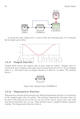
1.3.14 Product Block
It provides the product or division of two or more real input values. Each port can be
assigned only +1 or −1 value. +1 indicates that the corresponding input port performs
multiplication and −1 performs division in order of
y =
Q
i
Q
j
Here i represents to all the number inputs at product input ports. While j represents to
all the number inputs at division input ports. Port data [1; 1; −1] represents to the three
input ports and first port is multiplicative port, second port is also a multiplicative port
and third port is divisive port.
Y
Figure 1.69: Product block (PRODUCT)
1.3.15 Power Block
A function f = ua
is called power of u to a times. u is the supplied value and a is fixed
power that can be set accordingly. The value of a may be positive or negative. It has
only one input port and one output port. Note that, there shall be error if there is zero
crossing for negative power or output is an imaginary number. The reason is than
√
−2
Arun
1.3.14 Product Block
1.3.14 Product Block
t provides the product or division of two or more real input values. Each port can be
t provides the product or division of two or more real input values. Each port can be
Umrao
t provides the product or division of two or more real input values. Each port can be
t provides the product or division of two or more real input values. Each port can be](https://image.slidesharecdn.com/xcosscilabblockdescriptionswithsuitableexamples-211010151413/85/Notes-and-Description-for-Xcos-Scilab-Block-Simulation-with-Suitable-Examples-by-Arun-Umrao-82-320.jpg)


![The extraction of the line indices [1 2] and column indices [1 2], the extracted matrix
shall be
B =](https://image.slidesharecdn.com/xcosscilabblockdescriptionswithsuitableexamples-211010151413/85/Notes-and-Description-for-Xcos-Scilab-Block-Simulation-with-Suitable-Examples-by-Arun-Umrao-124-320.jpg)


Notes and Description for Xcos Scilab Block Simulation with Suitable Examples by Arun Umrao
- 1. 1 XCOS BLOCK DESCRIPTION A SIMPLE NOTES Arun Umrao www.sites.google.com/view/arunumrao DRAFT COPY - GPL LICENSING Arun Umrao
- 2. 2 Contents I Xcos Blocks 5 1 Blocks Pallets 7 1.1 Source of Data Blocks . . . . . . . . . . . . . . . . . . . . . . . . . . . . . 7 1.1.1 Clock Block . . . . . . . . . . . . . . . . . . . . . . . . . . . . . . . 7 1.1.2 Sampling Clock . . . . . . . . . . . . . . . . . . . . . . . . . . . . . 8 1.1.3 Time Function . . . . . . . . . . . . . . . . . . . . . . . . . . . . . 9 1.1.4 Constant Block . . . . . . . . . . . . . . . . . . . . . . . . . . . . . 10 1.1.5 Curve Block . . . . . . . . . . . . . . . . . . . . . . . . . . . . . . . 11 1.1.6 Counter Block . . . . . . . . . . . . . . . . . . . . . . . . . . . . . 12 1.1.7 Sine Wave Generator . . . . . . . . . . . . . . . . . . . . . . . . . . 14 1.1.8 Square Wave Generator . . . . . . . . . . . . . . . . . . . . . . . . 15 1.1.9 Saw-tooth Wave Generator . . . . . . . . . . . . . . . . . . . . . . 15 1.1.10 Pulse Wave Generator . . . . . . . . . . . . . . . . . . . . . . . . . 16 1.1.11 Step Function . . . . . . . . . . . . . . . . . . . . . . . . . . . . . . 17 1.1.12 Modulo Counter . . . . . . . . . . . . . . . . . . . . . . . . . . . . 18 1.1.13 Ramp . . . . . . . . . . . . . . . . . . . . . . . . . . . . . . . . . . 19 1.1.14 Random Generator . . . . . . . . . . . . . . . . . . . . . . . . . . . 19 1.1.15 Read From Input File . . . . . . . . . . . . . . . . . . . . . . . . . 20 1.1.16 Read ‘C’ Binary File . . . . . . . . . . . . . . . . . . . . . . . . . . 24 1.1.17 Read Sound File . . . . . . . . . . . . . . . . . . . . . . . . . . . . 26 1.1.18 Signal Builder . . . . . . . . . . . . . . . . . . . . . . . . . . . . . . 27 1.1.19 TK Scale . . . . . . . . . . . . . . . . . . . . . . . . . . . . . . . . 27 1.2 Sink of Data Blocks . . . . . . . . . . . . . . . . . . . . . . . . . . . . . . 28 1.2.1 Display Floating Number . . . . . . . . . . . . . . . . . . . . . . . 28 1.2.2 Bar XY . . . . . . . . . . . . . . . . . . . . . . . . . . . . . . . . . 28 1.2.3 Floating Point Scope . . . . . . . . . . . . . . . . . . . . . . . . . . 29 1.2.4 XY Animated Viewer . . . . . . . . . . . . . . . . . . . . . . . . . 29 1.2.5 XY 3D Animated Viewer . . . . . . . . . . . . . . . . . . . . . . . 30 1.2.6 3D Matrix Viewer . . . . . . . . . . . . . . . . . . . . . . . . . . . 31 1.2.7 Matrix Viewer . . . . . . . . . . . . . . . . . . . . . . . . . . . . . 33 1.2.8 Single Display Scope . . . . . . . . . . . . . . . . . . . . . . . . . . 38 1.2.9 Multiple Display Scope . . . . . . . . . . . . . . . . . . . . . . . . 40 1.2.10 XY Single Display Scope . . . . . . . . . . . . . . . . . . . . . . . 41 1.2.11 XY 3D Single Display Scope . . . . . . . . . . . . . . . . . . . . . 42 1.2.12 Terminating Blocks . . . . . . . . . . . . . . . . . . . . . . . . . . . 43 1.2.13 Writing to Audio File . . . . . . . . . . . . . . . . . . . . . . . . . 44 1.2.14 Writing to ‘C’ Binary File . . . . . . . . . . . . . . . . . . . . . . . 44 1.3 Mathematical Blocks . . . . . . . . . . . . . . . . . . . . . . . . . . . . . . 46 1.3.1 Max & Min . . . . . . . . . . . . . . . . . . . . . . . . . . . . . . . 46 1.3.2 Max Only Block . . . . . . . . . . . . . . . . . . . . . . . . . . . . 48 1.3.3 Min Only Block . . . . . . . . . . . . . . . . . . . . . . . . . . . . 48 1.3.4 Square Root Block . . . . . . . . . . . . . . . . . . . . . . . . . . . 48 1.3.5 Absolute Value . . . . . . . . . . . . . . . . . . . . . . . . . . . . . 49 Arun 1.1.15 Read From Input File . . . . . . . . . . . . . . . . . . . . . . . . . 20 1.1.15 Read From Input File . . . . . . . . . . . . . . . . . . . . . . . . . 20 1.1.16 Read ‘C’ Binary File . . . . . . . . . . . . . . . . . . . . . . . . . . 24 1.1.16 Read ‘C’ Binary File . . . . . . . . . . . . . . . . . . . . . . . . . . 24 1.1.17 Read Sound File . . . . . . . . . . . . . . . . . . . . . . . . . . . . 26 1.1.17 Read Sound File . . . . . . . . . . . . . . . . . . . . . . . . . . . . 26 Umrao 1.1.15 Read From Input File . . . . . . . . . . . . . . . . . . . . . . . . . 20 1.1.15 Read From Input File . . . . . . . . . . . . . . . . . . . . . . . . . 20 1.1.16 Read ‘C’ Binary File . . . . . . . . . . . . . . . . . . . . . . . . . . 24 1.1.16 Read ‘C’ Binary File . . . . . . . . . . . . . . . . . . . . . . . . . . 24 1.1.17 Read Sound File . . . . . . . . . . . . . . . . . . . . . . . . . . . . 26 1.1.17 Read Sound File . . . . . . . . . . . . . . . . . . . . . . . . . . . . 26
- 3. 3 1.3.6 Sum Function . . . . . . . . . . . . . . . . . . . . . . . . . . . . . . 50 1.3.7 Big Sum . . . . . . . . . . . . . . . . . . . . . . . . . . . . . . . . . 51 1.3.8 Summation Block . . . . . . . . . . . . . . . . . . . . . . . . . . . 52 1.3.9 Sine Function . . . . . . . . . . . . . . . . . . . . . . . . . . . . . . 52 1.3.10 Cosine Function . . . . . . . . . . . . . . . . . . . . . . . . . . . . 53 1.3.11 Tangent Function . . . . . . . . . . . . . . . . . . . . . . . . . . . . 54 1.3.12 Trigonometric Function . . . . . . . . . . . . . . . . . . . . . . . . 54 1.3.13 Product Function . . . . . . . . . . . . . . . . . . . . . . . . . . . . 55 1.3.14 Product Block . . . . . . . . . . . . . . . . . . . . . . . . . . . . . 56 1.3.15 Power Block . . . . . . . . . . . . . . . . . . . . . . . . . . . . . . 56 1.3.16 Exponential . . . . . . . . . . . . . . . . . . . . . . . . . . . . . . . 58 1.3.17 Gain of Function . . . . . . . . . . . . . . . . . . . . . . . . . . . . 59 1.3.18 Inverse Value . . . . . . . . . . . . . . . . . . . . . . . . . . . . . . 60 1.3.19 Logarithm Value . . . . . . . . . . . . . . . . . . . . . . . . . . . . 61 1.4 Matrix Blocks . . . . . . . . . . . . . . . . . . . . . . . . . . . . . . . . . . 61 1.4.1 Cumulative Summation . . . . . . . . . . . . . . . . . . . . . . . . 61 1.4.2 Extraction of Line & Column . . . . . . . . . . . . . . . . . . . . . 62 1.4.3 Triangular Or Triangular Extraction . . . . . . . . . . . . . . . . . 62 1.4.4 Horizontal Concatenation . . . . . . . . . . . . . . . . . . . . . . . 63 1.4.5 Vertical Concatenation . . . . . . . . . . . . . . . . . . . . . . . . . 64 1.4.6 Determinant . . . . . . . . . . . . . . . . . . . . . . . . . . . . . . 65 1.4.7 Diagonal . . . . . . . . . . . . . . . . . . . . . . . . . . . . . . . . . 65 1.4.8 Matrix Division . . . . . . . . . . . . . . . . . . . . . . . . . . . . . 66 1.4.9 Eigenvectors . . . . . . . . . . . . . . . . . . . . . . . . . . . . . . 67 1.4.10 Exponential Matrix . . . . . . . . . . . . . . . . . . . . . . . . . . 68 1.4.11 Inverse Matrix . . . . . . . . . . . . . . . . . . . . . . . . . . . . . 68 1.4.12 Lower & Upper Triangular Matrix (LU) . . . . . . . . . . . . . . . 69 1.4.13 Magnitude and Phi . . . . . . . . . . . . . . . . . . . . . . . . . . . 70 1.4.14 Matrix Multiplication . . . . . . . . . . . . . . . . . . . . . . . . . 70 1.4.15 Matrix Sum . . . . . . . . . . . . . . . . . . . . . . . . . . . . . . . 71 1.4.16 Matrix Transformation . . . . . . . . . . . . . . . . . . . . . . . . . 72 1.4.17 Conjugate Matrix . . . . . . . . . . . . . . . . . . . . . . . . . . . 73 1.4.18 Real & Imaginary Matrix . . . . . . . . . . . . . . . . . . . . . . . 73 1.4.19 Roots & Coefficients . . . . . . . . . . . . . . . . . . . . . . . . . . 74 1.4.20 Square Root of Matrix . . . . . . . . . . . . . . . . . . . . . . . . . 74 1.4.21 Sub Matrices . . . . . . . . . . . . . . . . . . . . . . . . . . . . . . 75 1.4.22 Riccati Equation . . . . . . . . . . . . . . . . . . . . . . . . . . . . 75 1.4.23 Singular Value Decomposition . . . . . . . . . . . . . . . . . . . . . 75 1.4.24 Pseudo Inverse Matrix . . . . . . . . . . . . . . . . . . . . . . . . . 80 1.4.25 Reshape Matrix . . . . . . . . . . . . . . . . . . . . . . . . . . . . . 80 1.5 Discrete & Continuum . . . . . . . . . . . . . . . . . . . . . . . . . . . . . 81 1.5.1 Backlash . . . . . . . . . . . . . . . . . . . . . . . . . . . . . . . . . 81 1.5.2 Deadband . . . . . . . . . . . . . . . . . . . . . . . . . . . . . . . . 82 1.5.3 Hystheresis . . . . . . . . . . . . . . . . . . . . . . . . . . . . . . . 83 1.5.4 Rate Limiter . . . . . . . . . . . . . . . . . . . . . . . . . . . . . . 83 1.5.5 Discrete Transfer Function . . . . . . . . . . . . . . . . . . . . . . 85 1.5.6 Discrete Zero Pole . . . . . . . . . . . . . . . . . . . . . . . . . . . 85 Arun 1.4.6 Determinant . . . . . . . . . . . . . . . . . . . . . . . . . . . . . . 65 1.4.6 Determinant . . . . . . . . . . . . . . . . . . . . . . . . . . . . . . 65 1.4.7 Diagonal . . . . . . . . . . . . . . . . . . . . . . . . . . . . . . . . . 65 1.4.7 Diagonal . . . . . . . . . . . . . . . . . . . . . . . . . . . . . . . . . 65 1.4.8 Matrix Division . . . . . . . . . . . . . . . . . . . . . . . . . . . . . 66 1.4.8 Matrix Division . . . . . . . . . . . . . . . . . . . . . . . . . . . . . 66 1.4.9 Eigenvectors . . . . . . . . . . . . . . . . . . . . . . . . . . . . . . 67 1.4.9 Eigenvectors . . . . . . . . . . . . . . . . . . . . . . . . . . . . . . 67 Umrao 1.4.6 Determinant . . . . . . . . . . . . . . . . . . . . . . . . . . . . . . 65 1.4.6 Determinant . . . . . . . . . . . . . . . . . . . . . . . . . . . . . . 65 1.4.7 Diagonal . . . . . . . . . . . . . . . . . . . . . . . . . . . . . . . . . 65 1.4.7 Diagonal . . . . . . . . . . . . . . . . . . . . . . . . . . . . . . . . . 65 1.4.8 Matrix Division . . . . . . . . . . . . . . . . . . . . . . . . . . . . . 66 1.4.8 Matrix Division . . . . . . . . . . . . . . . . . . . . . . . . . . . . . 66 1.4.9 Eigenvectors . . . . . . . . . . . . . . . . . . . . . . . . . . . . . . 67 1.4.9 Eigenvectors . . . . . . . . . . . . . . . . . . . . . . . . . . . . . . 67
- 4. 4 1.5.7 Discrete State Space System . . . . . . . . . . . . . . . . . . . . . 86 1.5.8 Shift Register . . . . . . . . . . . . . . . . . . . . . . . . . . . . . . 86 1.5.9 Dummy . . . . . . . . . . . . . . . . . . . . . . . . . . . . . . . . . 87 1.5.10 Continuous Transfer Function . . . . . . . . . . . . . . . . . . . . . 88 1.5.11 Continuous State Space System . . . . . . . . . . . . . . . . . . . . 88 1.5.12 Derivative . . . . . . . . . . . . . . . . . . . . . . . . . . . . . . . . 89 1.5.13 Integration . . . . . . . . . . . . . . . . . . . . . . . . . . . . . . . 90 1.5.14 PID Regulator . . . . . . . . . . . . . . . . . . . . . . . . . . . . . 91 1.5.15 Continuous Linear System With Jump . . . . . . . . . . . . . . . . 92 1.5.16 Unit Delay Operator . . . . . . . . . . . . . . . . . . . . . . . . . . 92 1.5.17 Continuous Time Delay . . . . . . . . . . . . . . . . . . . . . . . . 92 1.5.18 Discrete Time Delay . . . . . . . . . . . . . . . . . . . . . . . . . . 93 1.5.19 Variable Time Delay . . . . . . . . . . . . . . . . . . . . . . . . . . 94 1.5.20 Variable Time Delay Function . . . . . . . . . . . . . . . . . . . . 98 1.6 Electrical Blocks . . . . . . . . . . . . . . . . . . . . . . . . . . . . . . . . 98 1.6.1 Electrical Resistor . . . . . . . . . . . . . . . . . . . . . . . . . . . 99 1.6.2 Electrical Variable Resistor . . . . . . . . . . . . . . . . . . . . . . 100 1.6.3 Electrical Capacitor . . . . . . . . . . . . . . . . . . . . . . . . . . 101 1.6.4 Electrical Inductor . . . . . . . . . . . . . . . . . . . . . . . . . . . 102 1.6.5 Electrical DC Voltage Source . . . . . . . . . . . . . . . . . . . . . 103 1.6.6 Sine Wave Voltage Source . . . . . . . . . . . . . . . . . . . . . . . 104 1.6.7 Variable AC Voltage Source . . . . . . . . . . . . . . . . . . . . . . 105 1.6.8 Electrical AC Voltage Source . . . . . . . . . . . . . . . . . . . . . 105 1.6.9 Controllable Modelica Current Source . . . . . . . . . . . . . . . . 106 1.6.10 Controllable Modelica Voltage Source . . . . . . . . . . . . . . . . 107 1.6.11 Electrical Current Sensor . . . . . . . . . . . . . . . . . . . . . . . 107 1.6.12 Electrical Potential Sensor . . . . . . . . . . . . . . . . . . . . . . . 108 1.6.13 Electrical Voltage Sensor . . . . . . . . . . . . . . . . . . . . . . . 109 1.6.14 Electrical Diode . . . . . . . . . . . . . . . . . . . . . . . . . . . . 110 1.6.15 Ground . . . . . . . . . . . . . . . . . . . . . . . . . . . . . . . . . 111 1.6.16 Modelica Gyrator . . . . . . . . . . . . . . . . . . . . . . . . . . . . 112 1.6.17 Ideal Transformer . . . . . . . . . . . . . . . . . . . . . . . . . . . 113 1.6.18 Ideal OpAmp . . . . . . . . . . . . . . . . . . . . . . . . . . . . . . 113 1.6.19 PNP Transistor . . . . . . . . . . . . . . . . . . . . . . . . . . . . . 114 1.6.20 NPN Transistor . . . . . . . . . . . . . . . . . . . . . . . . . . . . . 114 1.6.21 Simple NMOS Transistor . . . . . . . . . . . . . . . . . . . . . . . 115 1.6.22 Simple PMOS Transistor . . . . . . . . . . . . . . . . . . . . . . . 115 1.6.23 NoN . . . . . . . . . . . . . . . . . . . . . . . . . . . . . . . . . . . 115 1.6.24 Input Zero Crossing . . . . . . . . . . . . . . . . . . . . . . . . . . 115 1.6.25 Zero Crossing General Block . . . . . . . . . . . . . . . . . . . . . 115 1.6.26 Negative to Positive Zero Crossing . . . . . . . . . . . . . . . . . . 116 1.6.27 Positive to Negative Zero Crossing . . . . . . . . . . . . . . . . . . 116 1.7 Signal Processing Blocks . . . . . . . . . . . . . . . . . . . . . . . . . . . . 117 1.7.1 Quantization . . . . . . . . . . . . . . . . . . . . . . . . . . . . . . 117 1.7.2 Sample And Hold . . . . . . . . . . . . . . . . . . . . . . . . . . . 118 1.7.3 Demultiplexer . . . . . . . . . . . . . . . . . . . . . . . . . . . . . . 119 1.7.4 Extractor . . . . . . . . . . . . . . . . . . . . . . . . . . . . . . . . 119 Arun 1.6.6 Sine Wave Voltage Source . . . . . . . . . . . . . . . . . . . . . . . 104 1.6.6 Sine Wave Voltage Source . . . . . . . . . . . . . . . . . . . . . . . 104 1.6.7 Variable AC Voltage Source . . . . . . . . . . . . . . . . . . . . . . 105 1.6.7 Variable AC Voltage Source . . . . . . . . . . . . . . . . . . . . . . 105 1.6.8 Electrical AC Voltage Source . . . . . . . . . . . . . . . . . . . . . 105 1.6.8 Electrical AC Voltage Source . . . . . . . . . . . . . . . . . . . . . 105 1.6.9 Controllable Modelica Current Source . . . . . . . . . . . . . . . . 106 1.6.9 Controllable Modelica Current Source . . . . . . . . . . . . . . . . 106 Umrao 1.6.6 Sine Wave Voltage Source . . . . . . . . . . . . . . . . . . . . . . . 104 1.6.6 Sine Wave Voltage Source . . . . . . . . . . . . . . . . . . . . . . . 104 1.6.7 Variable AC Voltage Source . . . . . . . . . . . . . . . . . . . . . . 105 1.6.7 Variable AC Voltage Source . . . . . . . . . . . . . . . . . . . . . . 105 1.6.8 Electrical AC Voltage Source . . . . . . . . . . . . . . . . . . . . . 105 1.6.8 Electrical AC Voltage Source . . . . . . . . . . . . . . . . . . . . . 105 1.6.9 Controllable Modelica Current Source . . . . . . . . . . . . . . . . 106 1.6.9 Controllable Modelica Current Source . . . . . . . . . . . . . . . . 106
- 5. 5 1.7.5 GOTO . . . . . . . . . . . . . . . . . . . . . . . . . . . . . . . . . . 120 1.7.6 FROM . . . . . . . . . . . . . . . . . . . . . . . . . . . . . . . . . . 120 1.7.7 GOTOMO . . . . . . . . . . . . . . . . . . . . . . . . . . . . . . . 121 1.7.8 FROMMO . . . . . . . . . . . . . . . . . . . . . . . . . . . . . . . 121 1.7.9 Scope Of GOTO . . . . . . . . . . . . . . . . . . . . . . . . . . . . 122 1.7.10 Scope Of GOTOMO . . . . . . . . . . . . . . . . . . . . . . . . . . 124 1.7.11 Clock Goto . . . . . . . . . . . . . . . . . . . . . . . . . . . . . . . 125 1.7.12 Clock From . . . . . . . . . . . . . . . . . . . . . . . . . . . . . . . 126 1.7.13 Select . . . . . . . . . . . . . . . . . . . . . . . . . . . . . . . . . . 126 1.7.14 Multiplexer . . . . . . . . . . . . . . . . . . . . . . . . . . . . . . . 127 1.7.15 Multi Port Switch . . . . . . . . . . . . . . . . . . . . . . . . . . . 128 1.7.16 Merge Data . . . . . . . . . . . . . . . . . . . . . . . . . . . . . . . 128 1.7.17 Relay . . . . . . . . . . . . . . . . . . . . . . . . . . . . . . . . . . 129 1.7.18 Select . . . . . . . . . . . . . . . . . . . . . . . . . . . . . . . . . . 129 1.7.19 Switch2 . . . . . . . . . . . . . . . . . . . . . . . . . . . . . . . . . 129 1.7.20 Switch . . . . . . . . . . . . . . . . . . . . . . . . . . . . . . . . . . 129 1.7.21 Self Switch . . . . . . . . . . . . . . . . . . . . . . . . . . . . . . . 130 1.8 User Defined Blocks . . . . . . . . . . . . . . . . . . . . . . . . . . . . . . 130 1.8.1 New C . . . . . . . . . . . . . . . . . . . . . . . . . . . . . . . . . . 130 Simulation Function . . . . . . . . . . . . . . . . . . . . . . . . . . 130 Is Block Implicit . . . . . . . . . . . . . . . . . . . . . . . . . . . . 130 Input Port Size . . . . . . . . . . . . . . . . . . . . . . . . . . . . . 131 Output Port Size . . . . . . . . . . . . . . . . . . . . . . . . . . . . 132 Input Event Size . . . . . . . . . . . . . . . . . . . . . . . . . . . . 133 Output Event Size . . . . . . . . . . . . . . . . . . . . . . . . . . . 133 Initial Continuous State . . . . . . . . . . . . . . . . . . . . . . . . 133 Number of Zero Crossing Surfaces . . . . . . . . . . . . . . . . . . 133 Initial Discrete State . . . . . . . . . . . . . . . . . . . . . . . . . . 133 Real Parameters Vector . . . . . . . . . . . . . . . . . . . . . . . . 133 Integer Parameters Vector . . . . . . . . . . . . . . . . . . . . . . . 133 Initial Firing Vector . . . . . . . . . . . . . . . . . . . . . . . . . . 134 Direct Feedthrough . . . . . . . . . . . . . . . . . . . . . . . . . . . 134 Time Dependence . . . . . . . . . . . . . . . . . . . . . . . . . . . 134 1.8.2 Masked Super Block . . . . . . . . . . . . . . . . . . . . . . . . . . 134 1.8.3 Mathematical Expression . . . . . . . . . . . . . . . . . . . . . . . 134 1.8.4 Modelica Generic Block . . . . . . . . . . . . . . . . . . . . . . . . 134 Input Variables . . . . . . . . . . . . . . . . . . . . . . . . . . . . . 135 Input Variables Types . . . . . . . . . . . . . . . . . . . . . . . . . 135 Output Variables . . . . . . . . . . . . . . . . . . . . . . . . . . . . 135 Output Variables Types . . . . . . . . . . . . . . . . . . . . . . . . 135 Parameters in Modelica . . . . . . . . . . . . . . . . . . . . . . . . 135 Parameters Properties . . . . . . . . . . . . . . . . . . . . . . . . . 136 Function name . . . . . . . . . . . . . . . . . . . . . . . . . . . . . 136 Parameter values . . . . . . . . . . . . . . . . . . . . . . . . . . . . 136 1.8.5 Super Block . . . . . . . . . . . . . . . . . . . . . . . . . . . . . . . 137 Ports for Connections in Super Block . . . . . . . . . . . . . . . . 139 Regular Input Port . . . . . . . . . . . . . . . . . . . . . . . . . . . 140 Arun Is Block Implicit . . . . . . . . . . . . . . . . . . . . . . . . . . . . 130 Is Block Implicit . . . . . . . . . . . . . . . . . . . . . . . . . . . . 130 Input Port Size . . . . . . . . . . . . . . . . . . . . . . . . . . . . . 131 Input Port Size . . . . . . . . . . . . . . . . . . . . . . . . . . . . . 131 Output Port Size . . . . . . . . . . . . . . . . . . . . . . . . . . . . 132 Output Port Size . . . . . . . . . . . . . . . . . . . . . . . . . . . . 132 Input Event Size . . . . . . . . . . . . . . . . . . . . . . . . . . . . 133 Input Event Size . . . . . . . . . . . . . . . . . . . . . . . . . . . . 133 Umrao Is Block Implicit . . . . . . . . . . . . . . . . . . . . . . . . . . . . 130 Is Block Implicit . . . . . . . . . . . . . . . . . . . . . . . . . . . . 130 Input Port Size . . . . . . . . . . . . . . . . . . . . . . . . . . . . . 131 Input Port Size . . . . . . . . . . . . . . . . . . . . . . . . . . . . . 131 Output Port Size . . . . . . . . . . . . . . . . . . . . . . . . . . . . 132 Output Port Size . . . . . . . . . . . . . . . . . . . . . . . . . . . . 132 Input Event Size . . . . . . . . . . . . . . . . . . . . . . . . . . . . 133 Input Event Size . . . . . . . . . . . . . . . . . . . . . . . . . . . . 133
- 6. 6 Regular Output Port . . . . . . . . . . . . . . . . . . . . . . . . . . 140 Implicit Input Port . . . . . . . . . . . . . . . . . . . . . . . . . . . 140 Implicit Output Port . . . . . . . . . . . . . . . . . . . . . . . . . . 141 Event Input Port . . . . . . . . . . . . . . . . . . . . . . . . . . . . 141 Event Output Port . . . . . . . . . . . . . . . . . . . . . . . . . . . 141 1.8.6 C Language . . . . . . . . . . . . . . . . . . . . . . . . . . . . . . . 141 Function Name . . . . . . . . . . . . . . . . . . . . . . . . . . . . . 142 Input Port Size . . . . . . . . . . . . . . . . . . . . . . . . . . . . . 143 Output Port Size . . . . . . . . . . . . . . . . . . . . . . . . . . . . 144 System Parameters Vector . . . . . . . . . . . . . . . . . . . . . . . 144 1.8.7 ForTran . . . . . . . . . . . . . . . . . . . . . . . . . . . . . . . . . 144 Function Name . . . . . . . . . . . . . . . . . . . . . . . . . . . . . 144 System parameters vector . . . . . . . . . . . . . . . . . . . . . . . 144 Input Port Size . . . . . . . . . . . . . . . . . . . . . . . . . . . . . 144 Output Port Size . . . . . . . . . . . . . . . . . . . . . . . . . . . . 145 1.8.8 Generic Block . . . . . . . . . . . . . . . . . . . . . . . . . . . . . . 145 Simulation Function . . . . . . . . . . . . . . . . . . . . . . . . . . 145 Function Type . . . . . . . . . . . . . . . . . . . . . . . . . . . . . 145 Input Port Size . . . . . . . . . . . . . . . . . . . . . . . . . . . . . 145 Input Port Type . . . . . . . . . . . . . . . . . . . . . . . . . . . . 146 Output Port Size . . . . . . . . . . . . . . . . . . . . . . . . . . . . 146 Output Port Type . . . . . . . . . . . . . . . . . . . . . . . . . . . 146 Input Port Event Size . . . . . . . . . . . . . . . . . . . . . . . . . 147 Output Port Event Size . . . . . . . . . . . . . . . . . . . . . . . . 147 Initial Continuous State . . . . . . . . . . . . . . . . . . . . . . . . 147 Initial Discrete State . . . . . . . . . . . . . . . . . . . . . . . . . . 147 Initial Object State . . . . . . . . . . . . . . . . . . . . . . . . . . 147 Real Parameters Vector . . . . . . . . . . . . . . . . . . . . . . . . 147 Integer Parameters Vector . . . . . . . . . . . . . . . . . . . . . . . 147 Object Parameters List . . . . . . . . . . . . . . . . . . . . . . . . 147 Number of Modes . . . . . . . . . . . . . . . . . . . . . . . . . . . 148 Number of Zero Crossing . . . . . . . . . . . . . . . . . . . . . . . 148 Initial Firing Vector . . . . . . . . . . . . . . . . . . . . . . . . . . 148 Direct Feed-through . . . . . . . . . . . . . . . . . . . . . . . . . . 148 Time Dependence . . . . . . . . . . . . . . . . . . . . . . . . . . . 148 1.8.9 Scilab Function Block . . . . . . . . . . . . . . . . . . . . . . . . . 148 Input Port Size . . . . . . . . . . . . . . . . . . . . . . . . . . . . . 148 Output Port Size . . . . . . . . . . . . . . . . . . . . . . . . . . . . 149 Input Event Port Size . . . . . . . . . . . . . . . . . . . . . . . . . 149 Output Event Port Size . . . . . . . . . . . . . . . . . . . . . . . . 149 Initial Continuous State . . . . . . . . . . . . . . . . . . . . . . . . 149 Initial Discrete State . . . . . . . . . . . . . . . . . . . . . . . . . . 149 System Parameter Vector . . . . . . . . . . . . . . . . . . . . . . . 149 Initial Firing Vector . . . . . . . . . . . . . . . . . . . . . . . . . . 149 Is Block Always Active . . . . . . . . . . . . . . . . . . . . . . . . 150 1.9 Other Blocks . . . . . . . . . . . . . . . . . . . . . . . . . . . . . . . . . . 150 1.9.1 Annotation . . . . . . . . . . . . . . . . . . . . . . . . . . . . . . . 150 Arun Output Port Size . . . . . . . . . . . . . . . . . . . . . . . . . . . . 146 Output Port Size . . . . . . . . . . . . . . . . . . . . . . . . . . . . 146 Output Port Type . . . . . . . . . . . . . . . . . . . . . . . . . . . 146 Output Port Type . . . . . . . . . . . . . . . . . . . . . . . . . . . 146 Input Port Event Size . . . . . . . . . . . . . . . . . . . . . . . . . 147 Input Port Event Size . . . . . . . . . . . . . . . . . . . . . . . . . 147 Output Port Event Size . . . . . . . . . . . . . . . . . . . . . . . . 147 Output Port Event Size . . . . . . . . . . . . . . . . . . . . . . . . 147 Umrao Output Port Size . . . . . . . . . . . . . . . . . . . . . . . . . . . . 146 Output Port Size . . . . . . . . . . . . . . . . . . . . . . . . . . . . 146 Output Port Type . . . . . . . . . . . . . . . . . . . . . . . . . . . 146 Output Port Type . . . . . . . . . . . . . . . . . . . . . . . . . . . 146 Input Port Event Size . . . . . . . . . . . . . . . . . . . . . . . . . 147 Input Port Event Size . . . . . . . . . . . . . . . . . . . . . . . . . 147 Output Port Event Size . . . . . . . . . . . . . . . . . . . . . . . . 147 Output Port Event Size . . . . . . . . . . . . . . . . . . . . . . . . 147
- 7. Part I Xcos Blocks Arun Umrao
- 8. Arun Umrao
- 9. 1.1. SOURCE OF DATA BLOCKS 9 1Blocks Pallets A Xcos model is created in the Xcos diagram panel. The diagram panel setup dialog can be opened by right clicking on the panel window and select of setup. From setup dialogue window we can set the final integration time (time upto which simulation takes place), real time scaling, Integrator absolute and relative tolerance (what amount of com- puted data shall be different from actual one), tolerance on time, maximum integration time interval, solver type and maximum step size etc. The same dialogue can be accessed from Setup submenu from Simulation menubar. From Xcos diagram panel and pallets we can create own simulating diagrams. There are ready-made blocks which are preinstall in Xcos. These blocks are called core Xcos blocks. There are few generic and user defined blocks through them we can access the other language in for analysis and computations. In xcos, familiarity with data type and port size is crucial for simulations. There are three main data arrangement in xcos. (i) Scalar data, (ii) Vector data and (iii) Matrix data. A scalar data is continuous data whose dimension always remains 1 × 1. Scalar data has infinite numbers of elements. Vector data is either of 1× n or m× 1 size. Vector data has fixed number of elements. A matrix data is always represented as m×n. It has also fixed number of elements. A function block accepts or transmits continuous data. A matrix block accepts or transmits vector or matrix data. To differentiate between function blocks and matrix blocks, their block name are ended with f and m (also contains MAT word in their block name) respectively. 1.1 Source of Data Blocks In Xcos, source blocks are those blocks where a pulse, signal or wave is generated. 1.1.1 Clock Block Clock block in Xcos is module that trigger pulses to another block. The maximum frequency of clock in Xcos is less than or equal to the processor frequency. The clock symbol is Figure 1.1: Clock (Clock c) This clock has one command port. In clock block, its frequency and initial time can be set as required. Following example uses the clock. Arun fixed number of elements. A matrix data is always represented as fixed number of elements. A matrix data is always represented as number of elements. A function block accepts or transmits continuous data. A matrix number of elements. A function block accepts or transmits continuous data. A matrix block accepts or transmits vector or matrix data. To differentiate between function blocks block accepts or transmits vector or matrix data. To differentiate between function blocks and matrix blocks, their block name are ended with and matrix blocks, their block name are ended with Umrao fixed number of elements. A matrix data is always represented as fixed number of elements. A matrix data is always represented as number of elements. A function block accepts or transmits continuous data. A matrix number of elements. A function block accepts or transmits continuous data. A matrix block accepts or transmits vector or matrix data. To differentiate between function blocks block accepts or transmits vector or matrix data. To differentiate between function blocks and matrix blocks, their block name are ended with and matrix blocks, their block name are ended with f and f and m (also contains MAT word m (also contains MAT word
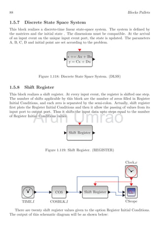
- 10. 10 Blocks Pallets Clock c CScope GenSin f Figure 1.2: In this configuration, a clock is used to refresh the single scope for showing the sine wave generated by sine function generator. The output will be like −10 −5 0 5 10 0 3 6 9 12 15 18 21 24 27 30 y t Figure 1.3: Output of simulation 1.2. A point to be noted that the period of clock is time period of one oscillation and its reverse is frequency of clock. T = 1 f ⇒ f = 1 T 1.1.2 Sampling Clock Another clock is sample clock whose frequency is calculated as greatest common divisor of all same offset blocks. Sampling clock has only one command port. Sampling rate and offset numbers can be set as required. Sampling rate is given in seconds, i.e. at each interval of this time, the clock send command signal to the connected block for reading of the input value. Offset value is that time after which the clock is activated. Arun Arun Umrao Umrao
- 11. 1.1. SOURCE OF DATA BLOCKS 11 Figure 1.4: Sampling Clock (SampleCLK) In the following example, a sampling clock is used with frequency of 5 seconds and offset time as 1 second. CScope GenSin f Figure 1.5: In this configuration, a sample clock is used to refresh the single scope for showing the sine wave generated by sine function generator. The output will be like −1 0 1 0 3 6 9 12 15 18 21 24 27 30 y t Figure 1.6: Output of simulation 1.5. 1.1.3 Time Function It is source of time. The data output at its output port is time increasing constantly by integer one. Figure 1.7: Time Function Block (TIME f) Figure 1.5: In this configuration, a sample clock is used to refresh the Figure 1.5: In this configuration, a sample clock is used to refresh the showing the sine wave generated by sine function generator. showing the sine wave generated by sine function generator. The output will be like The output will be like Umrao Figure 1.5: In this configuration, a sample clock is used to refresh the Figure 1.5: In this configuration, a sample clock is used to refresh the showing the sine wave generated by sine function generator. showing the sine wave generated by sine function generator.
- 12. 12 Blocks Pallets The time function is given as f(t) = t 0 ≤ t < ∞ Example for the time function is Clock c CScope TIME f Figure 1.8: In this configuration, a clock is used to refresh the single scope for showing the time function. Output of this example is −10 −5 0 5 10 0 3 6 9 12 15 18 21 24 27 30 y t Figure 1.9: Output of simulation 1.8. 1.1.4 Constant Block As named, constant block gives output a constant value. User can set the constant value as required. The constant symbol is 1 Figure 1.10: Constant Block (Const m) Arun Arun Arun Umrao Umrao
- 13. 1.1. SOURCE OF DATA BLOCKS 13 There are three types of constant block. Constant block (Const), constant block of function type (Const f) and constant block of matrix type (Const m). Constant block also accepts a vector or matrix as its value. For example, 1 5 5 −8 Figure 1.11: Constant Block (Const m) The schematic diagram of use of constant block is given below. Clock c CScope 3 Const m Figure 1.12: In this configuration, a clock is used to refresh the single scope for showing the constant value ‘3’. This simulation has output like −10 −8 −6 −4 −2 0 3 6 9 12 15 18 21 24 27 30 y t Figure 1.13: Output of simulation 1.12. 1.1.5 Curve Block Curve block plots user data into graphics window. It has one output port. User can modify xy-data from the setting option of the block. A graphical user interface is provided to edit Arun Arun Arun Arun Arun Arun Arun Arun Arun Arun Arun Arun Arun Arun Arun Arun Arun Arun Arun Arun Arun Arun Arun Arun Arun Arun Arun Arun Arun Arun Arun Arun Arun Arun Arun Arun Arun Arun Arun Arun Arun Arun Arun Arun Const Const m m Figure 1.12: In this configuration, a clock is used to refresh the single Figure 1.12: In this configuration, a clock is used to refresh the single Umrao Umrao Umrao Umrao Umrao Umrao Umrao Umrao Umrao Umrao Umrao Umrao Umrao Umrao Umrao Umrao Umrao Umrao Umrao Umrao Umrao Umrao Umrao Umrao Umrao Umrao Umrao Umrao Umrao Umrao Umrao Umrao Umrao Umrao Umrao Umrao Umrao Umrao Umrao Umrao Umrao Umrao Umrao Umrao CScope CScope Figure 1.12: In this configuration, a clock is used to refresh the single Figure 1.12: In this configuration, a clock is used to refresh the single scope for showing
- 14. 14 Blocks Pallets the xy-data. After completing the data it is required to save it to overwrite the previous data. Curve Figure 1.14: Curve Function Generator (CURV f) Clock c CScope Curve f This simulation has output like −10 −5 0 5 10 0 3 6 9 12 15 18 21 24 27 30 y t Figure 1.15: Output of simulation 1.1.5. 1.1.6 Counter Block Counter block counts from lower limit, normally 0, to upper limit (n) either in increasing order or in decreasing order as per user’s definition. Counter’s count (c) is controlled by clock, at each clock triger count value is changed by one. Normally control pulses are supplied by a clock. If clock frequency is low, counting is slow and if frequency of clock is high then counting is fast. User can set the properties of counter block. The counter symbol is Arun This simulation has output like This simulation has output like Arun Umrao
- 15. 1.1. SOURCE OF DATA BLOCKS 15 Counter 0 → n Figure 1.16: Counter block (Counter) Counter block simulation is given below Clock c CScope Counter 0 → 10 Counter Figure 1.17: In this configuration, a clock is used to refresh the single scope for showing the counter value from zero to fifteen. The counter value is reset to lower limit when count value is equal to the upper limit. Mathematically, c = ( c when c n 0 when c = n Or c = c % n This simulation has output like −10 −5 0 5 10 0 3 6 9 12 15 18 21 24 27 30 y t Figure 1.18: Output of simulation 1.17. Arun the counter value from zero to fifteen. the counter value from zero to fifteen. The counter value is reset to lower limit when count value is equal to the upper limit. The counter value is reset to lower limit when count value is equal to the upper limit. Mathematically, Mathematically, Umrao The counter value is reset to lower limit when count value is equal to the upper limit. The counter value is reset to lower limit when count value is equal to the upper limit.
- 16. 16 Blocks Pallets 1.1.7 Sine Wave Generator This block generates a sine wave of desired amplitude, frequency and initial time. Sine wave generated by this block has numerical relation as y = a sin ωt Amplitude, frequency and phase values can be set at the setting dialog of the block. The sine wave generator block is shown in below figure. Figure 1.19: Sine wave generator (GenSin f) Sine wave generator example is Clock c CScope GenSin f Figure 1.20: In this configuration, a clock is used to refresh the single scope for showing the sine wave. −1 0 1 0 1 2 3 4 5 6 7 8 Figure 1.21: Simulated output of simulation block (1.20). Arun Arun Umrao Umrao Umrao Umrao Umrao Umrao Umrao Umrao Umrao Umrao Umrao Umrao Umrao Umrao Umrao Umrao Umrao Umrao Umrao Umrao Umrao Umrao Umrao Umrao Umrao Umrao Umrao Umrao Umrao Umrao Umrao Umrao Umrao Umrao Umrao Umrao Umrao Umrao Umrao Umrao Umrao Umrao Umrao Umrao Umrao Umrao Umrao Umrao Umrao Umrao Umrao Umrao Umrao Umrao Umrao Umrao Umrao Umrao Umrao Umrao Umrao Umrao Umrao Umrao Umrao Umrao Umrao Umrao Umrao Umrao Umrao Umrao Umrao Umrao Umrao Umrao Umrao Umrao Umrao Umrao Umrao Umrao Umrao Umrao Umrao Umrao Umrao Umrao Umrao Umrao Umrao Umrao Umrao Umrao Umrao Umrao Umrao Umrao Umrao Umrao Umrao Umrao Umrao Umrao Umrao Umrao Umrao Umrao Umrao Umrao Umrao Umrao Umrao Umrao Umrao Umrao Umrao Umrao Umrao Umrao Umrao Umrao Umrao Umrao Umrao Umrao Umrao Umrao Umrao Umrao Umrao Umrao Umrao Umrao Umrao Umrao Umrao Umrao Umrao Umrao Umrao Umrao Umrao Umrao Umrao Umrao Umrao Umrao Umrao Umrao Umrao Umrao Umrao Umrao Umrao Umrao Umrao Umrao Umrao Umrao Umrao Umrao Umrao Umrao Umrao Umrao Umrao Umrao Umrao Umrao Umrao Umrao Umrao Umrao
- 17. 1.1. SOURCE OF DATA BLOCKS 17 1.1.8 Square Wave Generator Square wave generator produces a sinusoidal wave of square type. It has one control port and one output port. The width of square wave depends on the trigger pulse supplied by the clock through control port. A pulse trigger the lower level of square wave into upper level and vice-versa on next trigger pulse. Low frequency of trigger pulse (here a sinusoidal clock) gives larger width of square wave. Amplitude of square wave determines its height. Figure 1.22: Square Wave Generator (GENSQR f) Clock c CScope GENSQR f Figure 1.23: In this configuration, a clock is used to refresh the single scope for showing the square wave. Simulated output of circuit (1.23) is −1 0 1 0 1 2 3 4 5 6 7 8 1.1.9 Saw-tooth Wave Generator Sawtooth wave generator produces a wave whose shape is like a saw teeth. It has one control port and one output port. The shape is determined by the period of control pulse. Arun Arun Arun Arun Arun Arun Arun Arun Arun Arun Arun Arun Arun Arun Arun Arun Arun Arun Arun Arun Arun Arun Arun Arun Arun Arun Arun Arun Arun Arun Arun Arun Arun Arun Arun Arun Arun Arun Arun Arun Arun Arun Arun Arun Arun Arun Arun Arun Arun Arun Arun Arun Arun Arun Arun Arun Arun Arun Arun Arun Arun Arun Arun Arun Arun Arun Arun Arun Arun Arun Arun Arun Arun Arun Arun Arun Arun Arun Arun Arun Arun Arun Arun Arun Arun Arun Arun Arun Arun Arun Arun Arun Arun Arun Arun Arun Arun Arun Arun Arun Arun Arun Arun Arun Arun Arun Arun Arun Arun Arun Arun Arun Arun Arun Arun Arun Arun Arun Arun Arun Arun Arun Arun Arun Arun Arun Arun Arun Arun Arun Arun Arun Arun Arun Arun Arun Arun Arun Arun Arun Arun Arun Arun Arun Arun Arun Arun Arun Arun Arun Arun Arun Arun Arun Arun Arun Arun Arun Arun Arun Arun Arun Arun Arun Arun Arun Arun Arun Arun Arun Arun Arun Arun Arun Arun Arun Arun Arun Arun Arun Arun Arun Arun Arun Arun Arun Arun Arun Arun Arun Arun Arun Arun Arun Arun Arun Arun Arun Arun Arun Arun Arun Arun Arun Arun Arun Arun Arun Arun Arun Arun Arun Arun Arun Arun Arun Arun Arun Arun Arun Arun Arun Arun Arun Arun Arun Arun Arun Arun Arun Arun Arun Arun Arun Arun Arun Arun Arun Arun Arun Arun Arun Arun Arun Arun Arun Arun Arun Arun Arun Arun Arun Arun Arun Arun Arun Arun Arun Arun Arun Arun Arun Arun Arun Arun Arun Arun Arun Arun Arun Arun Arun Arun Arun Arun Arun Arun Arun Arun Arun Arun Arun Arun Arun Arun Arun Arun Arun Arun Arun Arun Arun Arun Arun Arun Arun Arun Arun Arun Arun Arun Arun Arun Arun Arun Arun Arun Arun Arun Arun Arun Arun Arun Arun Arun Arun Arun Arun Arun Arun Arun Arun Arun Arun Arun Arun Arun Arun Arun Arun Arun Arun Arun Arun Arun Arun Arun Arun Arun Arun Arun Arun Arun Arun Arun Arun Arun Arun Arun Arun Arun Arun Arun Arun Arun Arun Arun Arun Arun Arun Arun Arun Arun Arun Arun Arun Arun Arun Arun Arun Arun Arun Arun Arun Arun Arun Arun Arun Arun Arun Arun Arun Arun Arun Arun Arun Arun Arun Arun Arun Arun Arun Arun Arun Arun Arun Arun Arun Arun Arun Arun Arun Arun Arun Arun Arun Arun Arun Arun Arun Arun Arun Arun Arun Arun Arun Arun Arun Arun Arun Arun Arun Arun Arun Arun Arun Arun Arun Arun Arun Arun Arun Arun Arun Arun Arun Arun Arun Arun Arun Arun Arun Arun Arun Arun Arun Arun Arun Arun Arun Arun Arun Arun Arun Arun Arun Arun Arun Arun Arun Arun Arun Arun Arun Arun Arun Arun Arun Arun Arun Arun Arun Arun Arun Arun Arun Arun Arun Arun Arun Arun Arun Arun Arun Arun Arun Arun Arun Arun Arun Arun Arun Arun Arun Arun Arun Arun Arun Arun Arun Arun Arun Arun Arun Arun Arun Arun Arun Arun Arun Arun Arun Arun Arun Arun Arun Arun Arun Arun Arun Arun Arun Arun Arun Arun Arun Arun Arun Arun Arun Arun Arun Arun Arun Arun Arun Arun Arun Arun Arun Arun Arun Arun Arun Arun Arun Arun Arun Arun Arun Arun Arun Arun Arun Arun Arun Arun Arun Arun Arun Arun Arun Arun Arun Arun Arun Arun Arun Arun Arun Arun Arun Arun Arun Arun Arun Arun Arun Arun Arun Arun Arun Arun Arun Arun Arun Arun Arun Arun Arun Arun Arun Arun Arun Arun Arun Arun Arun Arun Arun Arun Arun Arun Arun Arun Arun Arun Arun Arun Arun Arun Arun Arun Arun Arun Arun Umrao Umrao Umrao Umrao Umrao Umrao Umrao Umrao Umrao Umrao Umrao Umrao Umrao Umrao Umrao Umrao Umrao Umrao Umrao Umrao Umrao Umrao Umrao Umrao Umrao Umrao Umrao Umrao Umrao Umrao Umrao Umrao Umrao Umrao Umrao Umrao Umrao Umrao Umrao Umrao Umrao Umrao Umrao Umrao Umrao Umrao Umrao Umrao Umrao Umrao Umrao Umrao Umrao Umrao Umrao Umrao Umrao Umrao Umrao Umrao Umrao Umrao Umrao Umrao Umrao Umrao Umrao Umrao Umrao Umrao Umrao Umrao Umrao Umrao Umrao Umrao Umrao Umrao Umrao Umrao Umrao Umrao Umrao Umrao Umrao Umrao Umrao Umrao Umrao Umrao Umrao Umrao Umrao Umrao Umrao Umrao Umrao Umrao Umrao Umrao Umrao Umrao Umrao Umrao Umrao Umrao Umrao Umrao Umrao Umrao Umrao Umrao Umrao Umrao Umrao Umrao Umrao Umrao Umrao Umrao Umrao Umrao Umrao Umrao Umrao Umrao Umrao Umrao Umrao Umrao Umrao Umrao Umrao Umrao Umrao Umrao Umrao Umrao Umrao Umrao Umrao Umrao Umrao Umrao Umrao Umrao Umrao Umrao Umrao Umrao Umrao Umrao Umrao Umrao Umrao Umrao Umrao Umrao Umrao Umrao Umrao Umrao Umrao Umrao Umrao Umrao Umrao Umrao Umrao Umrao Umrao Umrao Umrao Umrao Umrao Umrao Umrao Umrao Umrao Umrao Umrao Umrao Umrao Umrao Umrao Umrao Umrao Umrao Umrao Umrao Umrao Umrao Umrao Umrao Umrao Umrao Umrao Umrao Umrao Umrao Umrao Umrao Umrao Umrao Umrao Umrao Umrao Umrao Umrao Umrao Umrao Umrao Umrao Umrao Umrao Umrao Umrao Umrao Umrao Umrao Umrao Umrao Umrao Umrao Umrao Umrao Umrao Umrao Umrao Umrao Umrao Umrao Umrao Umrao Umrao Umrao Umrao Umrao Umrao Umrao Umrao Umrao Umrao Umrao Umrao Umrao Umrao Umrao Umrao Umrao Umrao Umrao Umrao Umrao Umrao Umrao Umrao Umrao Umrao Umrao Umrao Umrao Umrao Umrao Umrao Umrao Umrao Umrao Umrao Umrao Umrao Umrao Umrao Umrao Umrao Umrao Umrao Umrao Umrao Umrao Umrao Umrao Umrao Umrao Umrao Umrao Umrao Umrao Umrao Umrao Umrao Umrao Umrao Umrao Umrao Umrao Umrao Umrao Umrao Umrao Umrao Umrao Umrao Umrao Umrao Umrao Umrao Umrao Umrao Umrao Umrao Umrao Umrao Umrao Umrao Umrao Umrao Umrao Umrao Umrao Umrao Umrao Umrao Umrao Umrao Umrao Umrao Umrao Umrao Umrao Umrao Umrao Umrao Umrao Umrao Umrao Umrao Umrao Umrao Umrao Umrao Umrao Umrao Umrao Umrao Umrao Umrao Umrao Umrao Umrao Umrao Umrao Umrao Umrao Umrao Umrao Umrao Umrao Umrao Umrao Umrao Umrao Umrao Umrao Umrao Umrao Umrao Umrao Umrao Umrao Umrao Umrao Umrao Umrao Umrao Umrao Umrao Umrao Umrao Umrao Umrao Umrao Umrao Umrao Umrao Umrao Umrao Umrao Umrao Umrao Umrao Umrao Umrao Umrao Umrao Umrao Umrao Umrao Umrao Umrao Umrao Umrao Umrao Umrao Umrao Umrao Umrao Umrao Umrao Umrao Umrao Umrao Umrao Umrao Umrao Umrao Umrao Umrao Umrao Umrao Umrao Umrao Umrao Umrao Umrao Umrao Umrao Umrao Umrao Umrao Umrao Umrao Umrao Umrao Umrao Umrao Umrao Umrao Umrao Umrao Umrao Umrao Umrao Umrao Umrao Umrao Umrao Umrao Umrao Umrao Umrao Umrao Umrao Umrao Umrao Umrao Umrao Umrao Umrao Umrao Umrao Umrao Umrao Umrao Umrao Umrao Umrao Umrao Umrao Umrao Umrao Umrao Umrao Umrao Umrao Umrao Umrao Umrao Umrao Umrao Umrao Umrao Umrao Umrao Umrao Umrao Umrao Umrao Umrao Umrao Umrao Umrao Umrao Umrao Umrao Umrao Umrao Umrao Umrao Umrao Umrao Umrao Umrao Umrao Umrao Umrao Umrao Umrao Umrao Umrao Umrao Umrao Umrao Umrao Umrao Umrao Umrao Umrao Umrao Umrao Umrao Umrao Umrao
- 18. 18 Blocks Pallets It has slope of 450 and height and width of saw tooth depends on the period value of control pulse. The sawtooth wave generator block symbol is Figure 1.24: Saw-tooth Wave Generator (SAWTOOTH f) Clock c CScope SAWTOOTH f Figure 1.25: In this configuration, a clock is used to refresh the single scope for showing the saw-tooth wave. Simulated output of circuit (1.25) is −1 0 1 0 1 2 3 4 5 6 7 8 1.1.10 Pulse Wave Generator Pulse wave generator produces a square wave having different width in upper lower levels. It has one output port. The width of pulse wave can be defined by user as required. The pulse width is a fraction of period of the wave. Arun Figure 1.25: In this configuration, a clock is used to refresh the single Figure 1.25: In this configuration, a clock is used to refresh the single the saw-tooth wave. the saw-tooth wave. Umrao Figure 1.25: In this configuration, a clock is used to refresh the single Figure 1.25: In this configuration, a clock is used to refresh the single scope for showing scope for showing
- 19. 1.1. SOURCE OF DATA BLOCKS 19 Figure 1.26: Pulse Wave Generator (PULSE SC) The duration of time for which, the pulse wave remains active is known as “duty time”. Pulse width of the pulse wave is percentage ratio of the period of the wave. Clock c CScope PULSE SC Figure 1.27: In this configuration, a clock is used to refresh the single scope for showing of the pulse wave. Simulated output of circuit (1.27) is −1 0 1 2 0 1 2 3 4 5 6 7 8 1.1.11 Step Function Step function changes step from upper level to lower level or vice-versa. User can assign level change time and the upper lower level values (initial final values). The properties of this block are visible when it is double clicked. It has one output port. Figure 1.28: Step Function Generator (STEP FUNCTION) Arun Figure 1.27: In this configuration, a clock is used to refresh the single Figure 1.27: In this configuration, a clock is used to refresh the single of the pulse wave. of the pulse wave. Simulated output of circuit (1.27) is Simulated output of circuit (1.27) is Umrao Figure 1.27: In this configuration, a clock is used to refresh the single Figure 1.27: In this configuration, a clock is used to refresh the single scope for showing
- 20. 20 Blocks Pallets STEP FUNCTION is used to rise the level of value at and after any instant of time. Mathematically, step function is defined as givne below: f(t) = ( 0 when t a 1 when t ≥ a A simplest form of simulation circuit is shown in figure below. Clock c CScope STEP FUNCTION Figure 1.29: In this configuration, a clock is used to refresh the single scope for showing of the steps. Simulated output of circuit (1.29) is −1 0 1 2 0 1 2 3 4 5 6 7 8 1.1.12 Modulo Counter Counter modulo block counts the values, c, from zero to upper limit and when it encoun- ters to upper limit, it reset to zero. It has one control and one output ports. Counter Modulo n Figure 1.30: Counter Modulo block (Counter) Mathematically, modulo value c of given input i for upper limit n is represented as c = i mod n = i % n (1.1) Arun Simulated output of circuit (1.29) is Simulated output of circuit (1.29) is Umrao
- 21. 1.1. SOURCE OF DATA BLOCKS 21 Here, % sign is used to represent modulo in numerical programming. Modulo counter block simulation is given below Clock c CScope Counter Modulo 10 Modulo Counter Figure 1.31: In this configuration, a clock is used to refresh the single scope for showing the counter modulo 10. 1.1.13 Ramp Ramp block provide output values according to the relation y = mt + c Where y is value provided by ramp at any instant of time t. m, t c are ramp parameters. m is slope of ramp that determines how fast the output values varies. t is time function that increases continuously from its initial value. c is initial value of ramp output. Ramp has only one output port. Derivating to ramp relation m = dy dt The right side of above relation represent to velocity parameter, therefore, ramp function also represents to velocity function. The symbol of ramp function is Figure 1.32: Ramp block (Ramp) 1.1.14 Random Generator Random generator block generates random values within the two given ranges. The random value generated by this block is received when clock triggers the block. It has one control port and one output port. Mathematically r = R(t) where, r is sampled random value and R(t) is random value generated by the random block at time t. The random value r has range a ≤ r ≤ b, i.e. within domain of [a, b]. Arun is value provided by ramp at any instant of time is value provided by ramp at any instant of time is slope of ramp that determines how fast the output values varies. is slope of ramp that determines how fast the output values varies. Umrao mt + + c is value provided by ramp at any instant of time is value provided by ramp at any instant of time t. . m, , t t c c are ramp parameters. are ramp parameters. is slope of ramp that determines how fast the output values varies. is slope of ramp that determines how fast the output values varies. t t
- 22. 22 Blocks Pallets −2 −1 0 1 2 0 1 2 3 4 5 r t The block symbol is given below: Random Generator Figure 1.33: Random Generator block (Rand m) Each random block uses random number algorithm. User can defined own random block generator by using “Function Block”.. Clock c CScope Random Generator 1.1.15 Read From Input File This block is used to read data from input file stored in temporary directory or in “my document” folder. It has one control port and one output control port. Read data from input file Figure 1.34: Read from input file (RFILE f). This block uses configure options. 1. Time record selection : It is either an empty matrix or an strictly positive integer 0. If it is empty, there is no output event exists. If an integer value, ‘i’, is given, Arun block generator by using “Function Block”.. block generator by using “Function Block”.. Umrao block generator by using “Function Block”.. block generator by using “Function Block”.. Umrao Umrao Umrao Umrao Umrao Umrao Umrao Umrao Umrao Umrao Umrao Umrao Umrao Umrao Umrao Umrao Umrao Umrao Umrao Umrao Umrao Umrao Umrao Umrao Umrao Umrao Umrao Umrao Umrao Umrao Umrao Umrao Umrao Umrao Umrao Umrao Umrao Umrao Umrao Umrao Umrao Umrao Umrao Umrao Umrao Umrao Umrao Umrao Umrao Umrao Umrao Umrao Umrao Umrao Umrao Umrao Umrao Umrao Umrao Umrao Umrao Umrao Umrao Umrao Umrao Umrao Umrao Umrao Umrao Umrao Umrao Umrao Umrao Umrao Umrao Umrao Umrao Umrao Umrao Umrao Umrao Umrao Umrao Umrao Umrao Umrao Umrao Umrao Umrao Umrao Umrao Umrao Umrao Umrao Umrao Umrao Umrao Umrao Umrao Umrao Umrao Umrao Umrao Umrao Umrao Umrao Umrao Umrao Umrao Umrao Umrao Clock Clock c
- 23. 1.1. SOURCE OF DATA BLOCKS 23 then ith element of the read record is assumed to be the date of the output event, i.e. this record is treated as value of t-axis (time variable). 2. Outputs record selection : It is a vector of positive integers like [1, 2, 5]. If read data is like a vector [k1, k2, . . . kn] then kth i elements of the read records, i.e. the vector made of elements [k1, k2, k5] is given in output. 3. Input file name is a file name or path file name. Its value is string of characters. 4. Buffer size : It is similar to the number of bytes read by fread function of C language. To improve efficiency of input read, file is only done after each Buffer size call to the block. For example, consider a data file myfle.txt with following data except label row Arun Umrao
- 24. 24 Blocks Pallets C1 C2 C3 01 0.100 -0.100 02 0.199 -0.199 03 0.296 -0.296 04 0.389 -0.389 05 0.479 -0.479 06 0.565 -0.565 07 0.644 -0.644 08 0.717 -0.717 09 0.783 -0.783 10 0.841 -0.841 11 0.891 -0.891 12 0.932 -0.932 13 0.964 -0.964 14 0.985 -0.985 15 0.997 -0.997 16 1.000 -1.000 17 0.992 -0.992 18 0.974 -0.974 19 0.946 -0.946 20 0.909 -0.909 21 0.863 -0.863 22 0.808 -0.808 23 0.746 -0.746 24 0.675 -0.675 25 0.598 -0.598 26 0.516 -0.516 27 0.427 -0.427 28 0.335 -0.335 29 0.239 -0.239 30 0.141 -0.141 31 0.042 -0.042 32 -0.058 0.058 Each row has data record for different entity. Hence the unique data vector for each row is [k1, k2, k3]. If time record selection is 1, then first column will be used at t values, i.e. time event values. If this option has value 2, then second column is used at time even values. Note that, time value is always 0 and continuous increasing, hence block stops reading of data when either time becomes negative or time starts decreasing. So, time Arun 16 1.000 -1.000 17 1 18 0.974 -0.974 8 0.974 -0.974 Umrao 6 1.000 -1.000 6 1.000 -1.000 0. -0.992 8 0.974 -0.974 8 0.974 -0.974
- 25. 1.1. SOURCE OF DATA BLOCKS 25 column should be positive, greater than zero and continuous increasing. There are three output records. If output record selection has value 1 then only data of first column is sent as output of this block. If the output record selection has value [123] then values in first, second and third columns will be sent as output of this block. Clock c CScope Read data from input file RFILE f The time record selection is 1 and output record selection is [2, 3]. The output will be as −1 0 1 0 3 6 9 12 15 18 21 24 27 30 y t If the time record selection is 2 and output record selection is [2, 3], then time for data read shall be from t = 0 to t = 1 seconds. After than time starts decreasing hence reading block will stop reading of data from input data file. And the output will be as −1 0 1 0 3 6 9 12 15 18 21 24 27 30 y t If the time record selection is 3 and output record selection is [2, 3], then time for data read shall be from t = 0 to t = 0 seconds as time value is negative. There will be no output. Similarly, if time record selection option value is empty, then there is null time, hence no output. Arun Arun Arun Umrao Umrao Umrao
- 26. 26 Blocks Pallets −1 0 1 0 3 6 9 12 15 18 21 24 27 30 y t The ForTran data edit descriptors are LOGICAL, CHARACTER, INTEGER, REAL, DOUBLE PRECISION and COMPLEX which are represented by L, A, I, D, E, F or G descriptors respectively. ForTran descriptor is written as Iw.m where ‘I’ is data type, here it is integer, ‘w’ is total field width and it must be greater than zero, ‘m’ is minimum number of digits produced on output and it may be zero, ‘d’ is number of digits to the right of the decimal point and it may be zero, and ‘e’ number of digits in the exponent part and it must be greater than zero. ‘BN’ is blank space controller. While using this format control descriptor, all embedded and trailing blanks are treated as null and ignored. Similarly, in ‘BZ’ black control descriptor, all embedded and trailing blanks are treated as zeros. Blank space format control descriptor applies only to input and is ignored on output. ‘S’ format control descriptor restore the system default for printing plus ‘+’ signs. This is normally ‘SS’ which suppress the printing of plus ‘+’ signs in front of numerical data for the remainder of the FORMAT description. Format control descriptor ‘SP’ force the printing of plus ‘+’ signs in front of numerical data for the remainder of the FORMAT description. Plus sign format control descriptor are applies only to output and is ignored on input. There are column control descriptors in the ForTrans too. These are ‘nX’ which shifts right n spaces from current position. ‘Tn’ which shifts to column n in the record. ‘TLn’ which shifts left n spaces from current position. Note that you cannot shift left past column 1. This descriptor allows you to reread records on input and overwrite records on output. ‘TRn’ which shifts right n spaces from current position. Note that ‘TRn’ is exactly equivalent to ‘nX’. The slash ‘/’ descriptor begins a new line (record) on output and skips to the next line on input, ignoring any unread information on the current record. Two slashes ‘//’ skips one line, three slashes ‘///’ skips two lines, etc. The format descriptor may be repeated if it is defined as r(Fw.d) or r(Fw.d, Iw.d). Here, ‘r’ is an integer greater than one which specify, how many times the format descriptor inside the parentheses will be repeated. For example, 2(Fw.d) is equal to Fw.d, Fw.d. 1.1.16 Read ‘C’ Binary File This block is used to read ‘C’ binary file stored in temporary directory or in “my doc- ument” folder written by WRITEC f block. It has one control port and one output control port if Time Record Selection option has empty value. Otherwise, it also has one command port. Before reading this section, it is strongly recommended to read section explaining WRITEC f block. Arun data for the remainder of the FORMAT description. Format control descriptor ‘SP’ force data for the remainder of the FORMAT description. Format control descriptor ‘SP’ force the printing of plus ‘+’ signs in front of numerical data for the remainder of the FORMAT the printing of plus ‘+’ signs in front of numerical data for the remainder of the FORMAT description. Plus sign format control descriptor are applies only to output and is ignored description. Plus sign format control descriptor are applies only to output and is ignored on input. There are column control descriptors in the ForTrans too. These are ‘nX’ on input. There are column control descriptors in the ForTrans too. These are ‘nX’ Umrao data for the remainder of the FORMAT description. Format control descriptor ‘SP’ force data for the remainder of the FORMAT description. Format control descriptor ‘SP’ force the printing of plus ‘+’ signs in front of numerical data for the remainder of the FORMAT the printing of plus ‘+’ signs in front of numerical data for the remainder of the FORMAT description. Plus sign format control descriptor are applies only to output and is ignored description. Plus sign format control descriptor are applies only to output and is ignored on input. There are column control descriptors in the ForTrans too. These are ‘nX’ on input. There are column control descriptors in the ForTrans too. These are ‘nX’
- 27. 1.1. SOURCE OF DATA BLOCKS 27 Read from ‘C’ binary file Figure 1.35: Read from ‘C’ binary file (READC f). This block uses configure options. 1. Time Record Selection : It is either an empty matrix or an strictly positive integer greater than zero (scalar). If it is empty, there is no output event port exists. If an integer value, ‘i’, is given, then ith element of the read record is assumed to be the time event value of the output event port, i.e. this record is treated as value of t-axis (time variable). If this option has value greater than zero, then one command port is created in this block and ith will be used as time axis value and also may be used to control scope viewers. 2. Outputs Record Selection : It is a vector of positive integers like [1, 2, 5]. If read data is like a vector [k1, k2, . . . kn] then kth i elements of the read records, i.e. the vector made of elements [k1, k2, k5] is given in output. 3. Input File Name : It is a file name or path file name. Its value is string of characters. 4. Input Format : A character string defining the data format to use. Strings “l”, “i”, “s”, “ul”, “ui”, “us”, “d”, “f”, “c”, “uc” are used respectively to write int32, int16, int8, uint32, uint16, uint8, double, float, char or unsigned char data type. This value must be same as the value of Output Format option of WRITEC f block. 5. Record Size : This specify the number of columns to be read from C binary file. This should be same as the input size option of WRITEC f block. If this value is 2 and data being read from C binary file is integer type, then 8 bytes data shall be read for one record. It is vector of size one. 6. Buffer Size : It is similar to the number of bytes read by fread function of C language. 7. Initial Record Index : This fixes the first record of the file to use. For example, if record of each entity is arranged in one line and this option is set four, then file will be read from the fourth line in place of first line. 8. Swap Mode : If Swap mode=1 then file is supposed to be coded in “little endian IEEE format” and data are swapped if necessary to match the IEEE format of the processor. If Swap mode=0 then automatic bytes swap is disabled. A simple block arrangement is shown below: Arun 4. Input Format : A character string defining the data format to use. Strings “l”, “i”, 4. Input Format : A character string defining the data format to use. Strings “l”, “i”, “s”, “ul”, “ui”, “us”, “d”, “f”, “c”, “uc” are used respectively to write int32, int16, “s”, “ul”, “ui”, “us”, “d”, “f”, “c”, “uc” are used respectively to write int32, int16, int8, uint32, uint16, uint8, double, float, char or unsigned char data type. This int8, uint32, uint16, uint8, double, float, char or unsigned char data type. This Umrao 4. Input Format : A character string defining the data format to use. Strings “l”, “i”, 4. Input Format : A character string defining the data format to use. Strings “l”, “i”, “s”, “ul”, “ui”, “us”, “d”, “f”, “c”, “uc” are used respectively to write int32, int16, “s”, “ul”, “ui”, “us”, “d”, “f”, “c”, “uc” are used respectively to write int32, int16, int8, uint32, uint16, uint8, double, float, char or unsigned char data type. This int8, uint32, uint16, uint8, double, float, char or unsigned char data type. This
- 28. 28 Blocks Pallets Clock c CScope Read From c binary file READC f −1 0 1 0 3 6 9 12 15 18 21 24 27 30 y t If first column of read record is time value then Time Record Selection option shall have value 1. The block arrangement will be changed as CScope Read From c binary file READC f −1 0 1 0 3 6 9 12 15 18 21 24 27 30 y t 1.1.17 Read Sound File This block is used to read data sound file stored in temporary directory or in “my docu- ment” folder. It has one control port and one output control port. Arun have value 1. The block arrangement will be changed as have value 1. The block arrangement will be changed as Arun Arun Umrao have value 1. The block arrangement will be changed as have value 1. The block arrangement will be changed as Umrao Umrao
- 29. 1.1. SOURCE OF DATA BLOCKS 29 Read from .au sound file Figure 1.36: Read from sound file (READAU f). 1.1.18 Signal Builder Signal builder is used to draw a signals in any form as required. Signal builder uses x-y data for generating a signal. It has one output port and one command port. Signal Builder Figure 1.37: Signal Builder block (Sigbuilder) 1.1.19 TK Scale It is Tk powered slider scale window. Input value is adjusted by sliding the pointer of slider scale. This block has three parameters, (i) minimum value, (ii) maximum value and (iii) normalization. Normalization (h) controls the number of steps between minimum and maximum values. For example, if normalization is h, then total number of sliding steps shall be n = xmax − xmin h and vice-versa. Smaller the normalization value, larger the number of steps of Tk sliding scale and finer the input value. Hence there shall be larger steps and smaller normalization value for high precision input. Normalization is some times also known as step difference value of Tk sliding scale. This scale is used for tuning the signals. This block has one control port and one output port. TK Scale Figure 1.38: Signal Builder block (TKSCALE) Signals are stimulated by clock pulse. On stimulation, Tk slider scale supplies the value pointed by the pointer of the scale. Its minimum block requirement is shown below: Arun It is Tk powered slider scale window. Input value is adjusted by sliding the pointer of It is Tk powered slider scale window. Input value is adjusted by sliding the pointer of slider scale. This block has three parameters, (i) minimum value, (ii) maximum value slider scale. This block has three parameters, (i) minimum value, (ii) maximum value and (iii) normalization. Normalization ( and (iii) normalization. Normalization ( and maximum values. For example, if normalization is and maximum values. For example, if normalization is Umrao It is Tk powered slider scale window. Input value is adjusted by sliding the pointer of It is Tk powered slider scale window. Input value is adjusted by sliding the pointer of slider scale. This block has three parameters, (i) minimum value, (ii) maximum value slider scale. This block has three parameters, (i) minimum value, (ii) maximum value ) controls the number of steps between minimum ) controls the number of steps between minimum and maximum values. For example, if normalization is and maximum values. For example, if normalization is h h, then total number of sliding , then total number of sliding
- 30. 30 Blocks Pallets Clock c CScope TK Scale This simulation has output like −10 −5 0 5 10 0 3 6 9 12 15 18 21 24 27 30 y t Figure 1.39: Output of simulation 1.1.19. 1.2 Sink of Data Blocks Sinks is that point where all data is ended in form of graphs, numerical values or event. Following sinks are used in Xcos. 1.2.1 Display Floating Number This block is used to show the output in numeric form rather than graphical representa- tion. It has one input port and one command port. 1.2.2 Bar XY This block uses relation y = f(x) to plot the data. Here x is independent value while y is a function of x. This block shows results in bar lines. Arun Arun Arun Arun Arun Arun 0 3 6 9 12 15 18 21 24 27 30 0 3 6 9 12 15 18 21 24 27 30 Arun Umrao Umrao Umrao Umrao Umrao Umrao 0 3 6 9 12 15 18 21 24 27 30 0 3 6 9 12 15 18 21 24 27 30
- 31. 1.2. SINK OF DATA BLOCKS 31 1.2.3 Floating Point Scope Floating point scope, shows output of floating points ranges between zero to one. It has one control port. The output viewed in this scope is y = (float)x Figure 1.40: Floating Point Scope (CFSCOPE) Following parameters of the block can be set as and when required. Color Set the number for color of output graph. Output Window Number Output windows are assigned an identification numbers for processing of data. By default it is ‘-1’. It means the window number will automatically assigned an ID. Apart from it, user defined ID can also be assigned to the window. Output Window Position Position of window tell the window that where it will posi- tioned after opening. By default it is positioned in center of screen. The xy-coordinates of window position are assigned like [x; y]. The coordinates are calculated from the top left corner of the screen of computer system. Output Window Sizes It determines the size of output window. The coordinates are syntax as [x; y]. Ymin It is the minimum value of the output to be displayed in the output window. Ymin is used to set the lower scale point of the y-axis in output display. YMax It is the maximum value of the output to be displayed in the output window. Ymax is used to set the upper scale point of the y-axis in output display. Refresh Period It is the maximum range of independent variable to be displayed in the output window. Buffer Size The size of output values to be stored in the memory. The drawing is only done after each Buffer size call to the block. 1.2.4 XY Animated Viewer XY animated viewer visualized the second input with respect first input as a function of first input at instant simulated time. Mathematically y = f(x) The output plot is two dimensional. It has two input ports and one control port. One of the two input ports is for variable and second is for function of variable. Arun Output Window Position Output Window Position Position of window tell the window that where it will posi- Position of window tell the window that where it will posi- ioned after opening. By default it is positioned in center of screen. The xy-coordinates ioned after opening. By default it is positioned in center of screen. The xy-coordinates of window position are assigned like [ of window position are assigned like [ Umrao Position of window tell the window that where it will posi- Position of window tell the window that where it will posi- ioned after opening. By default it is positioned in center of screen. The xy-coordinates ioned after opening. By default it is positioned in center of screen. The xy-coordinates y]. The coordinates are calculated from the top ]. The coordinates are calculated from the top
- 32. 32 Blocks Pallets Figure 1.41: XY Animation Viewer block (CANIMXY) The simplest form of block arrangement is given in the following figure. Clock c CANIMXY TIME f SIN SINBLK f A moving dot is used to show the instantaneous x and y value. It is animated like the figure given below: −1 −0.5 0 0.5 1.0 0 1 2 3 4 5 6 7 1.2.5 XY 3D Animated Viewer XY 3D animated viewer block draw a graph of function like f(z) = f(x, y) Where x, y are two independent values. The α and φ values can be defined as required by user to change the viewing point. This block has one control port and three input ports. Figure 1.42: XY 3D Animated Viewer block (CANIMXY3D) The simplest form of block arrangement is given in the following figure. Arun A moving dot is used to show the instantaneous A moving dot is used to show the instantaneous figure given below: figure given below: Umrao A moving dot is used to show the instantaneous A moving dot is used to show the instantaneous x and y value. It is animated like the
- 33. 1.2. SINK OF DATA BLOCKS 33 Clock c CANIMXY3D TIME f SIN SINBLK f A moving dot is used to show the instantaneous x, y and z values. It is animated like the figure given below: x y z 1.2.6 3D Matrix Viewer 3D Matrix Viewer is a scope that shows matrix values as z values on a xy grid. It has one input port and one control port. The input to this block is always a matrix. Mat 3D Figure 1.43: 3D Matrix Viewer block (CMAT3D) The drawing of block arrangement is shown in the following figure. Clock c Mat 3D Mat. 3D 1 2 1 2 1 1 2 3 1 Arun Arun Arun Arun y y Arun Umrao Umrao Umrao Umrao Umrao Umrao Umrao Umrao Umrao Umrao Umrao Umrao Umrao
- 34. 34 Blocks Pallets Simulate this block arrangement to see the result. The output is computed as following methods. In CMAT3D matrix viewer, a ruled mess grid is created. Each point where x and y lines intersects to each other is called a node. At these nodes matrix elements are placed and element value is the height of the point in z-axis. The nodes parallel to the x-axis are column elements of the supplied matrix and nodes parallel to the y-axis are row elements of the supplied matrix. For a given matrix of 3 × 3, A = 1 2 1 2 1 1 2 3 1 The mess is looked like x y z The index of row or column numbers in CMAT3D viewer is started from zero. So, the elements of the matrix will be placed as shown in the following figure. Note that, column elements are placed parallel to the x-axis. Now, x y z A00 A10 A20 A01 A11 A21 A02 A12 A22 1 2 1 2 1 1 2 3 1 Now connect the zij from its neighbouring z. Four neighbouring z nodes form a facet of the 3D surface. The mesh thus form is three dimensional plot of the given function. Arun elements of the matrix will be placed as shown in the following figure. Note that, column elements of the matrix will be placed as shown in the following figure. Note that, column elements are placed parallel to the elements are placed parallel to the x x-axis. Now, -axis. Now, Umrao elements of the matrix will be placed as shown in the following figure. Note that, column elements of the matrix will be placed as shown in the following figure. Note that, column -axis. Now, -axis. Now,
- 35. 1.2. SINK OF DATA BLOCKS 35 x y z A00 A10 A20 A01 A11 A21 A02 A12 A22 1 2 1 2 1 1 2 3 1 Now, fill each quadrilateral surface with different color or using colormaps. This is output of the CMAT3D viewer block. x y z A00 A10 A20 A01 A11 A21 A02 A12 A22 1 2 1 2 1 1 2 3 1 1.2.7 Matrix Viewer Matrix Viewer is a scope that shows matrix values on colormap grid. It has one input port and one control port. The input to this block is always a matrix. The colormap grid is a range color linked to the window output of the scope. There are three types of color maps, (i) jetcolormap, (ii) hotcolormap and (iii) graycolormap. These colormaps accepts a level (n) of color map and it constructs color levels of size n × 3 where n ≥ 3. For example, 1 -- graycolormap (10) divides white to perfect gray color into ten different gray color shades as shown in the following output. ans = 0. 0. 0. 0.1111111 0.1111111 0.1111111 0.2222222 0.2222222 0.2222222 0.3333333 0.3333333 0.3333333 0.4444444 0.4444444 0.4444444 0.5555556 0.5555556 0.5555556 0.6666667 0.6666667 0.6666667 Arun Arun Arun Arun 1 Arun Umrao Umrao A00 A00 Umrao A10 A10 Umrao Umrao Umrao Umrao Umrao Umrao Umrao Umrao Umrao Umrao Umrao Umrao
- 36. 36 Blocks Pallets 0.7777778 0.7777778 0.7777778 0.8888889 0.8888889 0.8888889 1. 1. 1. Each shade contains equal components of red, green and blue colors. Hence rgb(0.1 0.1 0.1) is equal to the gray(0.1). All rgb components are zero means perfect black and all component of rgb are one means perfect white. The difference between two gray shades is computed as d = 1 − 0 n − 1 and levels are l = 0 + i × d The minimum level range is the minimum value who comes in the regular input port. It would be linked to the ‘cold value’ of the colormap. The maximum level range is the maximum value who comes in the regular input port. It would be linked to the ‘hot value’ of the colormap. Minimum and maximum values are scalars. Mat View Figure 1.44: Matrix Viewer block (CMATVIEW) The drawing of block arrangement is shown in the following figure. Clock c Mat View 0. 1. 2. 2. 3. 4. 4. 5. 6. 6. 7. 8. Computation method of this block is explained as given below. Assume that the input matrix has elements from minimum value 0 to maximum value 8. There are eight levels of gray colourmap. So the list of actual gray colourmap codes, those will be used to fill the plot are 1 -- graycolourmap (8) ans = 0. 0.1428571 0.2857143 Arun F Figure 1.44: Matrix Viewer block (CMATVIEW) igure 1.44: Matrix Viewer block (CMATVIEW) Umrao igure 1.44: Matrix Viewer block (CMATVIEW) igure 1.44: Matrix Viewer block (CMATVIEW)
- 37. 1.2. SINK OF DATA BLOCKS 37 0.4285714 0.5714286 0.7142857 0.8571429 1. Let the matrix elements are arranged in the xy-plane taking x-axis as rows and y-axis as columns. The experimental matrix is 1 -- M=[0 1 2; 2 3 4; 4 5 6;6 7 8] M= 0. 1. 2. 2. 3. 4. 4. 5. 6. 6. 7. 8. Now, the minimum matrix value (say 0) is set to gray color level 0 and maximum matrix value (say 8) is set to gray color level 1. The intermediate distinct matrix elements are assigned proposed gray color code from equally distributed gray colormap values ranging from 0 to 1 as shown in the below table. Matrix Element Proposed Gray Code 0 0.000 1 0.125 2 0.250 3 0.375 4 0.500 5 0.625 6 0.750 7 0.875 8 1.000 As there are 8 colormap levels and 9 distinct matrix elements, hence the proposed gray color codes are rounded to near gray colormap values of actual gray colormap. Thus the actual table will be Arun Matrix Elemen Umrao Proposed Gray Code 0.000
- 38. 38 Blocks Pallets Elements Proposed Gray Code Actual Gray Code 0 0.000 0.000 1 0.125 0.143 2 0.250 0.286 3 0.375 0.429 4 0.500 0.571 5 0.625 0.714 6 0.750 0.857 7 0.875 1.000 8 1.000 1.000 The matrix nodes are as cols rows (0,0.000) (1,0.143) (2,0.286) (2,0.286) (3,0.429) (4,0.571) (4,0.571) (5,0.714) (6,0.857) (6,0.857) (7,1.000) (8,1.000) These matrix arrangement creates grid blocks/cells as shown below: cols rows (0,0.000) (1,0.143) (2,0.286) (2,0.286) (3,0.429) (4,0.571) (4,0.571) (5,0.714) (6,0.857) (6,0.857) (7,1.000) (8,1.000) Arun Arun (1,0.143) (3,0.429) (3,0.429) Umrao (5,0.714) (5,0.714) (7,1.000) (7,1.000)
- 39. 1.2. SINK OF DATA BLOCKS 39 Now, for each cell, its corner values are used for calculation of average gray scale for that cell. So, the first cell has gray value as g = 0.000 + 0.286 + 0.143 + 0.429 4 = 0.2145 cols rows (0,0.000) (1,0.143) (2,0.286) (2,0.286) (3,0.429) (4,0.571) (4,0.571) (5,0.714) (6,0.857) (6,0.857) (7,1.000) (8,1.000) 0.215 The shading of this cell be like cols rows (0,0.000) (1,0.143) (2,0.286) (2,0.286) (3,0.429) (4,0.571) (4,0.571) (5,0.714) (6,0.857) (6,0.857) (7,1.000) (8,1.000) 0.215 Now, we can calculate average gray scales/levels for other cells and their background can be filled by appropriate gray colors as shown in the following figure. Arun (0,0.000) 0,0.000) (2,0.286) The shading of this cell be like The shading of this cell be like Umrao (4,0.571) (4,0.571) (6,0.857)
- 40. 40 Blocks Pallets cols rows (0,0.000) (1,0.143) (2,0.286) (2,0.286) (3,0.429) (4,0.571) (4,0.571) (5,0.714) (6,0.857) (6,0.857) (7,1.000) (8,1.000) 0.215 0.500 0.785 0.357 0.642 0.892 1.2.8 Single Display Scope Single display scope displays its input with respect to simulation time. User can change the refresh time, maximum and minimum value of axes. It has one control port and one input port. Figure 1.45: Single Display Scope (CSCOPE) This scope can be customized from the setting dialogue which can be opened by double clicking one it. The default input size of this scope is 8, i.e. data vector size shall be less than or equal to ‘8’. The color is a vector of integers. The ith element is the color number or marker type used to draw the evolution of the ith input port signal. Colors are defined by positive integers i.e. color index relative to the current colormap and markers are defined by negative integers. The marker type are identified by an integer in range of 0 to -14 which stands respectively for: dot, plus, cross, star, filled diamond, diamond, triangle up, triangle down, diamond plus, circle, asterisk, square, triangle right, triangle left and pentagram. Note that, this scope automatically detects the number of data groups coming inside and plots different/multiple plots in same graphics window. In the following figure, a sine wave is plotted at single scope window. Arun Umrao Umrao Umrao Umrao Umrao Umrao Umrao Umrao Umrao Umrao Umrao Umrao Umrao Umrao Umrao Umrao Umrao Umrao Umrao Umrao Umrao Umrao Umrao Umrao Umrao Umrao Umrao Umrao Umrao Umrao Umrao Umrao Umrao Umrao Umrao Umrao Umrao Umrao Umrao Umrao Umrao Umrao Umrao Umrao Umrao Umrao Umrao Umrao Umrao Umrao Umrao Umrao Umrao Umrao Umrao Umrao Umrao Umrao Umrao Umrao Umrao Umrao Umrao Umrao Umrao Umrao Umrao Umrao Umrao Umrao Umrao Umrao Umrao Umrao Umrao Umrao Umrao Umrao Umrao Umrao Umrao Umrao Umrao Umrao Umrao Umrao Umrao Umrao Umrao Umrao Umrao Umrao Umrao Umrao Umrao Umrao Umrao Umrao Umrao Umrao Umrao Umrao Umrao Umrao Umrao Umrao Umrao Umrao Umrao Umrao Umrao Umrao Umrao Umrao Umrao Umrao Umrao Umrao Umrao Umrao Umrao Umrao Umrao Umrao Umrao Umrao Umrao Umrao Umrao Umrao Umrao Umrao Umrao Umrao Umrao Umrao Umrao Umrao Umrao Umrao Umrao Umrao Umrao Umrao Umrao Umrao Umrao Umrao Umrao Umrao Umrao Umrao Umrao Umrao Umrao Umrao Umrao Umrao Umrao Umrao Umrao Umrao Umrao Umrao Umrao Umrao Umrao Umrao Umrao Umrao Umrao Umrao Umrao Umrao Umrao Umrao Umrao Umrao Umrao Umrao Umrao Umrao Umrao Umrao Umrao Umrao Umrao Umrao Umrao Umrao Umrao Umrao Umrao Umrao Umrao Umrao Umrao Umrao Umrao Umrao Umrao Umrao Umrao Umrao Umrao Umrao Umrao Umrao Umrao Umrao Umrao Umrao Umrao Umrao Umrao Umrao Umrao Umrao Umrao Umrao Umrao Umrao Umrao Umrao Umrao Umrao Umrao Umrao Umrao Umrao Umrao Umrao Umrao Umrao Umrao Umrao Umrao Umrao Umrao Umrao Umrao Umrao Umrao Umrao Umrao Umrao Umrao Umrao Umrao Umrao Umrao Umrao Umrao Umrao Umrao Umrao Umrao Umrao Umrao Umrao Umrao Umrao Umrao Umrao Umrao Umrao Umrao Umrao Umrao Umrao Umrao Umrao Umrao Umrao Umrao Umrao Umrao Umrao Umrao Umrao Umrao Umrao Umrao Umrao Umrao Umrao Umrao Umrao Umrao Umrao Umrao Umrao Umrao Umrao Umrao Umrao Umrao Umrao Umrao Umrao Umrao Umrao Umrao Umrao Umrao Umrao Umrao Umrao Umrao Umrao Umrao Umrao Umrao Umrao Umrao Umrao Umrao Umrao Umrao Umrao Umrao Umrao Umrao Umrao Umrao Umrao Umrao Umrao Umrao Umrao Umrao Umrao Umrao Umrao Umrao Umrao Umrao Umrao Umrao Umrao Umrao Umrao Umrao Umrao Umrao Umrao Umrao Umrao Umrao Umrao Umrao Umrao Umrao Umrao Umrao Umrao Umrao Umrao Umrao Umrao Umrao Umrao Umrao Umrao Umrao Umrao Umrao Umrao Umrao Umrao Umrao Umrao Umrao Umrao Umrao Umrao Umrao Umrao Umrao Umrao Umrao Umrao Umrao Umrao Umrao Umrao Umrao Umrao Umrao Umrao Umrao Umrao Umrao Umrao Umrao Umrao Umrao Umrao Umrao Umrao Umrao Umrao Umrao Umrao Umrao Umrao Umrao Umrao Umrao Umrao Umrao Umrao Umrao Umrao Umrao Umrao Umrao Umrao Umrao Umrao Umrao Umrao Umrao Umrao Umrao Umrao Umrao Umrao Umrao Umrao Umrao Umrao Umrao Umrao Umrao Umrao Umrao Umrao Umrao Umrao Umrao Umrao Umrao Umrao Umrao Umrao Umrao Umrao Umrao Umrao Umrao Umrao Umrao Umrao Umrao Umrao Umrao Umrao Umrao Umrao Umrao Umrao Umrao Umrao Umrao Umrao Umrao Umrao Umrao Umrao Umrao Umrao Umrao Umrao Umrao Umrao Umrao Umrao Umrao Umrao Umrao Umrao Umrao Umrao Umrao Umrao Umrao Umrao Umrao Umrao Umrao Umrao Umrao Umrao Umrao Umrao Umrao Umrao Umrao Umrao Umrao Umrao Umrao Umrao Umrao Umrao Umrao Umrao Umrao Umrao Umrao Umrao Umrao Umrao Umrao Umrao Umrao Umrao Umrao Umrao Umrao Umrao Umrao Umrao Umrao Umrao Umrao Umrao Umrao Umrao Umrao Umrao Umrao Umrao Umrao Umrao Umrao Umrao Umrao Umrao Umrao Umrao Umrao Umrao Umrao Umrao Umrao Umrao Umrao Umrao Umrao Umrao Umrao Umrao Umrao Umrao Umrao Umrao Umrao Umrao Umrao Umrao Umrao Umrao Umrao Umrao Umrao Umrao Umrao Umrao Umrao Umrao Umrao Umrao Umrao Umrao Umrao Umrao Umrao Umrao Umrao Umrao Umrao Umrao
- 41. 1.2. SINK OF DATA BLOCKS 41 Clock c CScope GenSin f The output will be like −2 −1 0 1 2 0 3 6 9 12 15 18 21 24 27 30 y t For grouping of multiple data, Multiplexure is used. In the following figure, two sine wave data is multiplexed before passing it to input port of single scope viewer. Here both data are plotted in same graph window as shown in the output. Clock c CScope GenSin f GenSin f The output will be like Arun Arun Arun Arun Arun Arun 3 6 9 12 15 18 21 24 27 30 3 6 9 12 15 18 21 24 27 30 Umrao Umrao Umrao Umrao Umrao Umrao Umrao Umrao 3 6 9 12 15 18 21 24 27 30 3 6 9 12 15 18 21 24 27 30
- 42. 42 Blocks Pallets −2 −1 0 1 2 0 3 6 9 12 15 18 21 24 27 30 y t 1.2.9 Multiple Display Scope Multiple display scope displays its different input values simultaneously with respect to simulation time . User can change the refresh time, number of input port its size and type, maximum and minimum value of axes for each input ports and buffer size etc. The size of input port of the multiple display scope should be equal to the size of data received from the output port of other block. It accepts continuous data or row matrix or column matrix or vector data types. For continuous data type, input port size is 1, and for row or column matrix or vector data, the input port size is size of row or column matrix or vector. The size of input port is set accordingly. Matrix data of m × n type can not be directly fed to this display scope. It has one control port and user defined multiple input port. This scope draws subplots in different subgraphics windows for each input port data. Figure 1.46: Multiple Display Scope (CMSCOPE) For the input ports of this block, user must be familiar with size of the ports and type of the ports. For example, in the field ‘input port sizes’ in setting dialogue, if data is placed as ‘1 1’ then it represents to two input ports as ‘1’ is written two times separated with space. Similarly, ‘1 1 1’ represents to three input ports. ‘1 2 1’ is also represents to three input ports but these ports are of different type. ‘1’ represents that a port can receives or transmits only one column vector (1 × 1 vector), which is also known as continuous scalar data. While ‘2’ represents that a port can receives or transmits only two column vector (1 × 2 vector). It is also known as row matrix data. Similarly ‘7’ represents a vector having seven columns (1 × 7 vector) and so on. Remember that a Scope needs the drawing color equal to the sum of size of all ports. If there are two ports of size 3 and 7 respectively, then there is required to define 3+7 = 10 colours in ‘Drawing colors or marks’ field. There are also required to set the separate values of Ymin, Ymax and refresh rate for each input port. Arun matrix or vector data types. For continuous data type, input port size is 1, and for row matrix or vector data types. For continuous data type, input port size is 1, and for row or column matrix or vector data, the input port size is size of row or column matrix or or column matrix or vector data, the input port size is size of row or column matrix or vector. The size of input port is set accordingly. Matrix data of vector. The size of input port is set accordingly. Matrix data of directly fed to this display scope. It has one control port and user defined multiple input directly fed to this display scope. It has one control port and user defined multiple input Umrao matrix or vector data types. For continuous data type, input port size is 1, and for row matrix or vector data types. For continuous data type, input port size is 1, and for row or column matrix or vector data, the input port size is size of row or column matrix or or column matrix or vector data, the input port size is size of row or column matrix or vector. The size of input port is set accordingly. Matrix data of vector. The size of input port is set accordingly. Matrix data of m m × n n directly fed to this display scope. It has one control port and user defined multiple input directly fed to this display scope. It has one control port and user defined multiple input
- 43. 1.2. SINK OF DATA BLOCKS 43 Clock c CScope GenSin f GenSin f The output will be like −2 −1 0 0 3 6 9 12 15 18 21 24 27 30 −2 −1 0 0 3 6 9 12 15 18 21 24 27 30 1.2.10 XY Single Display Scope This block visualize the two inputs signals by drawing the second input as a function of the first input at any instant of time. When a point is drawn on screen it stays until the simulation is finished. It has two input ports and one control ports. One of the two input ports is for variable and second is for function of variable. y = f(x) Figure 1.47: XY Single Display Scope (CSCOPXY) The simplest form of block arrangement is given in the following figure. Arun Arun Umrao Umrao
- 44. 44 Blocks Pallets Clock c CSCOPXY TIME f SIN SINBLK f A moving dot with trailing curve is used to show the animated path. It is animated like the figure given below: −1 −0.5 0 0.5 1.0 0 1 2 3 4 5 6 7 1.2.11 XY 3D Single Display Scope This block visualize the two inputs signals by drawing the second input as a function of the first input at any instant of time. When a point is drawn on screen it stays until the simulation is finished. It has two input ports and one control ports. Two of the three input ports are for variables and third is for function of variables. The mathematics behind the visualization is f(z) = f(x, y) Figure 1.48: XY 3D Single Display Scope (CSCOPXY3D) The simplest form of block arrangement is given in the following figure. Arun 0 1 2 1.2.11 XY 3D Single Display Scope 1.2.11 XY 3D Single Display Scope Umrao 3 3 4 5 6 7 1.2.11 XY 3D Single Display Scope 1.2.11 XY 3D Single Display Scope
- 45. 1.2. SINK OF DATA BLOCKS 45 Clock c CSCOPXY3D TIME f SIN SINBLK f A moving dot with trailing curve is used to show the animated path. It is animated like the figure given below: x y z 1.2.12 Terminating Blocks A terminating block ends the simulation when simulation time is encounter to the time specified in terminating blocks. There are three types of terminating blocks. First is ‘End Block’: it ends the simulation after the time specified in the end block. It has no ports. END Figure 1.49: End Block (ENDBLK) Second type of terminating block is ending counter. It received current time from control port and matches with defined final time in itself. If both are equal, it instructs final simulation time otherwise passes current time from command port. This block has one control port and one command port. END Figure 1.50: End Block (END c) Arun Arun Arun Arun y y Arun Arun Umrao Umrao Umrao Umrao
- 46. 46 Blocks Pallets Third is halt block. HALT Figure 1.51: Halt Block (HALT f) Some times, there is situation when one or more ports are need to keep open but simulation can not be processed if one or more ports are hanging. So to keep these ports close we use trash block. It just make port close and all the data received at this port is considered as junk. This block works as terminating blocks and do nothing. Trash Figure 1.52: Trash Function block (TRASH f) 1.2.13 Writing to Audio File This block writes the sound data in *.au file format. It has one control port and one input port. Generally file is saved in the same directory where *.xcos file is saved but user can change the name and path of the writing file. Before using this block, user must have writing permissions. Write to audio Figure 1.53: Write AU to devaudio (WRITEAU f) 1.2.14 Writing to ‘C’ Binary File This block writes the data in binary ‘C’ file. It has one control port and one input port. Generally file is saved in the same directory where *.xcos file is saved but user can change the name and path of the writing file. Before using this block, user must have writing permissions. Write to C Figure 1.54: Write To Binary ‘C’ (WRITEC f) Arun .2.13 Writing to Audio File .2.13 Writing to Audio File This block writes the sound data in *.au file format. It has one control port and one This block writes the sound data in *.au file format. It has one control port and one input port. Generally file is saved in the same directory where *.xcos file is saved but input port. Generally file is saved in the same directory where *.xcos file is saved but Umrao This block writes the sound data in *.au file format. It has one control port and one This block writes the sound data in *.au file format. It has one control port and one input port. Generally file is saved in the same directory where *.xcos file is saved but input port. Generally file is saved in the same directory where *.xcos file is saved but
- 47. 1.2. SINK OF DATA BLOCKS 47 1. Input Size : It is size of input column vector. A scalar that determines the how many columns of data values are used to form a record. This description must be read with the data output format description. Suppose, we have define integer datatype data format and input size is 2 then total 8 bytes shall be used to write a record of data in binary form. The data received at input port of WRITEC f block must be of same size as defined in the Input Size option. 2. Output File Name : It is a file name or path file name where data would be written. Its value is string of characters. 3. Output Format : A character string defining the data format to use. Strings “l”, “i”, “s”, “ul”, “ui”, “us”, “d”, “f”, “c”, “uc” are used respectively to write int32, int16, int8, uint32, uint16, uint8, double, float, char or unsigned char data type. 4. Buffer Size : It is similar to the number of bytes read by fread function of C language. 5. Swap Mode : If swap mode=1 then file is supposed to be coded in “little endian IEEE format” and data are swapped if necessary to match the IEEE format of the processor. If Swap mode=0 then automatic bytes swap is disabled. Clock c Write to C GenSin f The above block diagram is indicative purpose about the use of WRITEC f. The data written by this block is in format as shown below: rec[4] 20 4 byte[1] byte[2] rec[5] 40 12 byte[1] byte[2] rec[6] 60 20 byte[1] byte[2] rec[7] 80 28 byte[1] byte[2] wr In this figure, we have explained that the character type data with size two is saved in binary format. First byte is for one of the two data elements of a record and second byte is for other of the two data elements of a record. The number of bytes required depends on the type of data and size of data. A character data type requires one byte memory space and if record size is two then two bytes are required to save a record. If data type is integer type and data size is two, then memory arrangement shall be like rec[4] 0 0 20 4 byte[1] byte[2] byte[3] byte[4] rec[5] 0 0 40 12 byte[1] byte[2] byte[3] byte[4] rec[6] 0 0 60 20 byte[1] byte[2] byte[3] byte[4] wr Arun Umrao Umrao Umrao Umrao Umrao Umrao Umrao Umrao Umrao Umrao Umrao Umrao Umrao Umrao Umrao Umrao Umrao Umrao Umrao Umrao Umrao Umrao Umrao Umrao Umrao Umrao Umrao Umrao Umrao Umrao Umrao Umrao Umrao Umrao Umrao Umrao Umrao Umrao Umrao Umrao Umrao Umrao Umrao Umrao Umrao Umrao Umrao Umrao Umrao Umrao Umrao Umrao Umrao Umrao Umrao Umrao Umrao Umrao Umrao Umrao Umrao Umrao Umrao Umrao Umrao Umrao Umrao Umrao Umrao Umrao Umrao Umrao Umrao Umrao Umrao Umrao Umrao Umrao Umrao Umrao Umrao Umrao Umrao Umrao Umrao Umrao Umrao Umrao Umrao Umrao Umrao Umrao Umrao Umrao Umrao Umrao Umrao Umrao Umrao Umrao Umrao Umrao Umrao Umrao Umrao Umrao Umrao Umrao Umrao Umrao Umrao Umrao Umrao Umrao Umrao Umrao Umrao Umrao Umrao Umrao Umrao Umrao Umrao Umrao Umrao Umrao Umrao Umrao Umrao Umrao Umrao Umrao Umrao Umrao Umrao Umrao Umrao Umrao Umrao Umrao Umrao Umrao Umrao Umrao Umrao Umrao Umrao Umrao Umrao Umrao Umrao Umrao Umrao Umrao Umrao Umrao Umrao Umrao Umrao Umrao Umrao Umrao Umrao Umrao Umrao Umrao Umrao Umrao Umrao Umrao Umrao Umrao Umrao Umrao Umrao Umrao Umrao Umrao Umrao Umrao Umrao Umrao Umrao Umrao Umrao Umrao Umrao Umrao Umrao Umrao Umrao Umrao Umrao Umrao Umrao Umrao Umrao Umrao Umrao Umrao Umrao Umrao Umrao Umrao Umrao Umrao Umrao Umrao Umrao Umrao Umrao Umrao Umrao Umrao Umrao Umrao Umrao Umrao Umrao Umrao Umrao Umrao Umrao Umrao Umrao Umrao Umrao Umrao Umrao Umrao Umrao Umrao Umrao Umrao Umrao Umrao Umrao Umrao Umrao Umrao Umrao Umrao Umrao Umrao Umrao Umrao Umrao Umrao Umrao Umrao Umrao Umrao Umrao Umrao Umrao Umrao Umrao Umrao Umrao Umrao Umrao Umrao Umrao Umrao Umrao Umrao Umrao Umrao Umrao Umrao Umrao Umrao Umrao Umrao Umrao Umrao Umrao Umrao Umrao Umrao Umrao Umrao Umrao Umrao Umrao Umrao Umrao Umrao Umrao Umrao Umrao Umrao Umrao Umrao Umrao Umrao Umrao Umrao Umrao Umrao Umrao Umrao Umrao Umrao Umrao Umrao Umrao Umrao Umrao Umrao Umrao Umrao Umrao Umrao Umrao Umrao Umrao Umrao Umrao Umrao Umrao Umrao Umrao Umrao Umrao Umrao Umrao Umrao Umrao Umrao Umrao Umrao Umrao Umrao Umrao Umrao Umrao Umrao Umrao Umrao Umrao Umrao Umrao Umrao Umrao Umrao Umrao Umrao Umrao Umrao Umrao Umrao Umrao Umrao Umrao Umrao Umrao Umrao Umrao Umrao
- 48. 48 Blocks Pallets Note that, index origin has been implemented in different programming languages differently. The equivalent decimal number in each memory byte represents the binary value saved in that memory cell. 1.3 Mathematical Blocks In this section, those blocks are discussed which are used in mathematical operations. 1.3.1 Max Min Max min block compares the two input values and returns the minimum or maximum value as the conditions are defined. This block can be used in vector mode only i.e. input should be supplied only vector values. If zero crossing is set true then negative value would also be returned. MAX Figure 1.55: Max-Min block (MAXMIN) This block acts as Min block if min/max input option is set to 1 and acts as Max block if min/max input option is set to 2. It may be set for one input or two inputs. A schematic diagram is shown for working of Max/Min block. Clock c CScope TIME f SIN SINBLK f TIME f COS COSBLK f MAX In this block two inputs, one sine value and other cosine value are entered into the max/min block. The block is set to max state, i.e. the maximum value of the two inputs will be found at its output port. Therefore, the final plot shall be plot of the maximum value between sine and cosine values. The time clock starts from 0 to continue. The number of input ports in max/min block is set to two and zero crossing is allowed. The output of this schematic diagram will be as shown below: Arun This block acts as Min block if min/max input option is set to 1 and acts as Max This block acts as Min block if min/max input option is set to 1 and acts as Max block if min/max input option is set to 2. It may be set for one input or two inputs. A block if min/max input option is set to 2. It may be set for one input or two inputs. A Umrao This block acts as Min block if min/max input option is set to 1 and acts as Max This block acts as Min block if min/max input option is set to 1 and acts as Max block if min/max input option is set to 2. It may be set for one input or two inputs. A block if min/max input option is set to 2. It may be set for one input or two inputs. A
- 49. 1.3. MATHEMATICAL BLOCKS 49 −1 −0.5 0 0.5 1.0 0 3 6 9 12 15 18 21 24 27 30 −1 −0.5 0 0.5 1.0 0 3 6 9 12 15 18 21 24 27 30 −1 −0.5 0 0.5 1.0 0 3 6 9 12 15 18 21 24 27 30 When the max/min block is set to minimum state, the output of updated configured schematic block diagram will be as shown below: −1 −0.5 0 0.5 1.0 0 3 6 9 12 15 18 21 24 27 30 −1 −0.5 0 0.5 1.0 0 3 6 9 12 15 18 21 24 27 30 −1 −0.5 0 0.5 1.0 0 3 6 9 12 15 18 21 24 27 30 Arun When the max/min block is set to minimum state, the output of updated When the max/min block is set to minimum state, the output of updated schematic block diagram will be as shown below: schematic block diagram will be as shown below: Umrao When the max/min block is set to minimum state, the output of updated When the max/min block is set to minimum state, the output of updated schematic block diagram will be as shown below: schematic block diagram will be as shown below:
- 50. 50 Blocks Pallets 1.3.2 Max Only Block Max block returns the maximum value of all supplied values. Max block can be used in matrix mode of input data. It has only one input port and one output port. The max block is MAX Figure 1.56: Max block (MAX f) If A =
- 56. 4 8 6 9 1 12 4 7 3
- 62. is input to this block then it gives 12 as its output. The value 12 is maximum among all elements of the given matrix. 1.3.3 Min Only Block Min block returns the minimum value of all supplied values. Min block can be used in matrix mode of input data. It has only one input port and one output port. Min block is MIN Figure 1.57: Min block (MIN f) If A =
- 68. 4 8 6 9 1 12 4 7 3
- 74. is input to this block then it gives 1 as its output. The value 1 is minimum among all elements of the given matrix. 1.3.4 Square Root Block A function f(x) = √ x is called square root function of x. The type of roots can be set by user. It has only one input port and one output port. SQRT Figure 1.58: Square root block (SQRT) Arun Min block returns the minimum value of all supplied values. Min block can be used in Min block returns the minimum value of all supplied values. Min block can be used in matrix mode of input data. It has only one input port and one output port. Min block is matrix mode of input data. It has only one input port and one output port. Min block is Umrao Min block returns the minimum value of all supplied values. Min block can be used in Min block returns the minimum value of all supplied values. Min block can be used in matrix mode of input data. It has only one input port and one output port. Min block is matrix mode of input data. It has only one input port and one output port. Min block is
- 75. 1.3. MATHEMATICAL BLOCKS 51 If square root block is set to real only (data type = 1) then it gives output when input is only positive value as √ −n is an imaginary value. There is NULL result if input is a negative number. It can also be set to complex mode by changing its data type to 2 in setting dialogue. 1.3.5 Absolute Value Absolute value is mod value of a real number. If given number is positive or negative its absolute value is always positive in nature. The absolute block returns only positive form of a positive or negative real number. The absolute block is ABS Figure 1.59: Absolute value block (ABS VALUE) Mathematically f(x) = −a when a 0 a when a ≥ 0 A schematic diagram is shown for working of absolute block. Clock c CScope TIME f COS COSBLK f ABS The output of this schematic diagram will be as shown below: Arun A schematic diagram is shown for working of absolute block. A schematic diagram is shown for working of absolute block. Umrao A schematic diagram is shown for working of absolute block. A schematic diagram is shown for working of absolute block.
- 76. 52 Blocks Pallets −1 −0.5 0 0.5 1.0 0 3 6 9 12 15 18 21 24 27 30 −1 −0.5 0 0.5 1.0 0 3 6 9 12 15 18 21 24 27 30 1.3.6 Sum Function It provides the sum of three input values algebraically without changing the nature of input values. This block accepts input values as they are supplied. It has three input ports and one output port. M Figure 1.60: Sum function block (SUM f) If f(x), g(x) and h(x) are three inputs for the function, then it gives result y = f(x) + g(x) + h(x) Clock c CScope TIME f SIN SINBLK f TIME f COS COSBLK f M The output of this schematic diagram will be as shown below: Arun Umrao Umrao Umrao Umrao M M
- 77. 1.3. MATHEMATICAL BLOCKS 53 −1 −0.5 0 0.5 1.0 0 3 6 9 12 15 18 21 24 27 30 −1 −0.5 0 0.5 1.0 0 3 6 9 12 15 18 21 24 27 30 −2 −1.5 −1.0 −0.5 0 0.5 1.0 1.5 2.0 0 3 6 9 12 15 18 21 24 27 30 1.3.7 Big Sum It provides the sum of two or more real input values algebraically either by accepting them as they are or by changing their nature. User can change the number of input. It has unlimited input ports and one output port. Number of input ports depends on the input port matrix. Each element in port matrix represents one input port. The numerical value of each element is the gain of input values. Gain of input port ranges from 0 to ∞. For example [0; 1; −2] represents to the three input ports and first port has zero gain, second port has +1 gain and third port has −2 gain1 . X Figure 1.61: Big sum block (BIGSOM f) The additive or subtractive nature of input port can be assigned by using plus or minus sign in port matrix. If both signs are assigned to the input ports then their additive or subtractive nature of input ports are shown by plus or minus sign. 1 Gain is defined as the ratio of final value to the initial value Arun Arun Umrao Umrao
- 78. 54 Blocks Pallets + - X Figure 1.62: Big sum block (BIGSOM f) If α, β and γ are three gains of the three inputs of the big sum and their input values are i, j and k respectively, then the result output of this function shall be algebraic sum of the product input port gain and their corresponding inputs. y = αi + βj + γj This is obsolete block. 1.3.8 Summation Block It provides the sum of two or more input vector values algebraically. User can change the number of input ports. It unlimited input ports and one output port. Input ports can be assigned only either +1 or −1 values i.e. [1; −1; 1; 1; 1] etc. The gain of input values is only 1 in factor. + - X Figure 1.63: Summation block (SUMMATION) The principal difference between big sum block and summation block is that summa- tion block can add two or more real or imaginary or complex or int32 values. It also give warning or do nothing or shows saturated values when data overflows. 1.3.9 Sine Function Sine block returns the sine value of given angle (in radian). The maximum and minimum value of sine function lies between ±1. The initial value of sine function is 0 when θ = 0 radian. The sine block is SIN Figure 1.64: Sine block (SINBLK f) The simplest form of block arrangement is given in the following figure. Arun Umrao Umrao Umrao Umrao Umrao Umrao Umrao Umrao Umrao Umrao Umrao Umrao Umrao Umrao Umrao Umrao Umrao Umrao Umrao Umrao Umrao Umrao Umrao Umrao Umrao Umrao Umrao Umrao Umrao Umrao Umrao Umrao Umrao Umrao Umrao Umrao Umrao Umrao Umrao Umrao Umrao Umrao Umrao Umrao Umrao Umrao Umrao Umrao Umrao Umrao Umrao Umrao Umrao Umrao Umrao Umrao Umrao Umrao Umrao Umrao Umrao Umrao Umrao Umrao Umrao Umrao Umrao Umrao Umrao Umrao Umrao Umrao Umrao Umrao Umrao Umrao Umrao Umrao Umrao Umrao Umrao Umrao Umrao Umrao Umrao Umrao Umrao Umrao Umrao Umrao Umrao Umrao Umrao Umrao Umrao Umrao Umrao Umrao Umrao Umrao Umrao Umrao Umrao Umrao Umrao Umrao Umrao Umrao Umrao Umrao Umrao Umrao Umrao Umrao Umrao Umrao Umrao Umrao Umrao Umrao Umrao Umrao Umrao Umrao Umrao Umrao Umrao Umrao Umrao Umrao Umrao Umrao Umrao Umrao Umrao Umrao Umrao Umrao Umrao Umrao Umrao Umrao Umrao Umrao Umrao Umrao Umrao Umrao Umrao Umrao Umrao Umrao Umrao Umrao Umrao Umrao Umrao Umrao Umrao Umrao Umrao Umrao Umrao Umrao Umrao Umrao Umrao Umrao Umrao Umrao Umrao Umrao Umrao Umrao Umrao Umrao Umrao Umrao Umrao Umrao Umrao Umrao Umrao Umrao Umrao Umrao Umrao Umrao Umrao Umrao Umrao Umrao Umrao Umrao Umrao Umrao Umrao Umrao Umrao Umrao Umrao Umrao Umrao Umrao Umrao Umrao Umrao Umrao Umrao Umrao Umrao Umrao Umrao Umrao Umrao Umrao Umrao Umrao Umrao Umrao Umrao Umrao Umrao Umrao Umrao Umrao Umrao Umrao Umrao Umrao Umrao Umrao Umrao Umrao Umrao Umrao + + + + + + + + + + + + + + + + + + + + + + + + + + + + + + + + + + + + + + Umrao X X X X X X X X X X X X X X X X X X X X X X X X X X X X X X X X X X X X X X X X X X X X X X X X X X X X X X X X X X
- 79. 1.3. MATHEMATICAL BLOCKS 55 Clock c CSCOPXY TIME f SIN SINBLK f A moving dot with trailing curve is used to show the animated path. It is animated like the figure given below: −1 −0.5 0 0.5 1.0 0 1 2 3 4 5 6 7 1.3.10 Cosine Function Cosine block returns the cosine value of given angle (in radian). The maximum and minimum value of cosine function lies between ±1. The initial value of cosine function is +1 when θ = 0 radian. The function plot of cosine leads to the plot of sine function by π/2 radian. The cosine block is looked like COS Figure 1.65: Cosine block (COSBLK f) The simplest form of block arrangement is given in the following figure. Arun 0 1 2 1.3.10 Cosine Function 1.3.10 Cosine Function Umrao 3 3 4 5 6 7
- 80. 56 Blocks Pallets Clock c CSCOPXY TIME f COS COSBLK f A moving dot with trailing curve is used to show the animated path. It is animated like the figure given below: −1 −0.5 0 0.5 1.0 0 1 2 3 4 5 6 7 1.3.11 Tangent Function Tangent block returns the tangent value of given angle (in radian). Tangent value in- creases from zero to infinity when angle value increases from zero to π/2. At pi/2 tangent value is ∞. The initial value of tangent function is 0 when θ = 0 radian. The absolute block is TAN Figure 1.66: Tangent block (TANBLK f) 1.3.12 Trigonometric Function Trigonometric function block provides user defined trigonometric function to be operated on the supplied angle value (in radian). The auxiliary trigonometric functions those can be used in this block are any of the sin, cos, tan, arcsin, arccos, arctan, sinh, cosh, tanh and inverse hyperbolic sin, cos, tan. Only function name is supplied without argument variable. The trigonometric function block is 0 1 2 1.3.11 Tangent Function 1.3.11 Tangent Function Umrao 3 3 4 5 6 7
- 81. 1.3. MATHEMATICAL BLOCKS 57 Trig Functions Figure 1.67: Trigonometric Function block (TrigFun) 1.3.13 Product Function It provides the product of two input values altering input values. This block accepts input values as they are supplied. It has two input ports and one output port. O Figure 1.68: Product function block (PROD f) If f(x), g(x) and h(x) are three inputs for the function, then result of product block is y = f(x) × g(x) × h(x) Clock c CScope TIME f SIN SINBLK f TIME f COS COSBLK f O The output of this schematic diagram will be as shown below: Arun y f Arun Arun Umrao ) ) × g( (x x) × h(x)
- 82. 58 Blocks Pallets −1 −0.5 0 0.5 1.0 0 3 6 9 12 15 18 21 24 27 30 −1 −0.5 0 0.5 1.0 0 3 6 9 12 15 18 21 24 27 30 −1 −0.5 0 0.5 1.0 0 3 6 9 12 15 18 21 24 27 30 1.3.14 Product Block It provides the product or division of two or more real input values. Each port can be assigned only +1 or −1 value. +1 indicates that the corresponding input port performs multiplication and −1 performs division in order of y = Q i Q j Here i represents to all the number inputs at product input ports. While j represents to all the number inputs at division input ports. Port data [1; 1; −1] represents to the three input ports and first port is multiplicative port, second port is also a multiplicative port and third port is divisive port. Y Figure 1.69: Product block (PRODUCT) 1.3.15 Power Block A function f = ua is called power of u to a times. u is the supplied value and a is fixed power that can be set accordingly. The value of a may be positive or negative. It has only one input port and one output port. Note that, there shall be error if there is zero crossing for negative power or output is an imaginary number. The reason is than √ −2 Arun 1.3.14 Product Block 1.3.14 Product Block t provides the product or division of two or more real input values. Each port can be t provides the product or division of two or more real input values. Each port can be Umrao t provides the product or division of two or more real input values. Each port can be t provides the product or division of two or more real input values. Each port can be
- 83. 1.3. MATHEMATICAL BLOCKS 59 gives imaginary output and 0−n gives undetermined value (1/0), i.e. division by zero or infinite value. u a Result 1 0.5 1.00 3 0.5 1.73 5 0.5 2.23 4 0.5 2.00 -2 0.5 Imaginary -3 -1.5 Imaginary 0 -1.5 Div by 0 -4 -2.0 0.0625 -6 -2.0 0.028 6 -2.0 0.028 Power block symbol is given below: ua Figure 1.70: Power block (POWBLK f) Minimum block arrangement for power block is given below: Clock c CScope ua TK Scale Figure 1.71: Minimum Block Arrangement. This simulation has output like Arun Power block symbol is given below: Power block symbol is given below: Umrao Umrao Umrao Umrao Umrao Umrao Umrao Umrao Umrao Umrao Umrao Umrao Umrao Umrao Umrao Umrao Umrao Umrao Umrao Umrao Umrao Umrao Umrao Umrao Umrao Umrao Umrao Umrao Umrao Umrao Umrao Umrao Umrao Umrao Umrao Umrao Umrao Umrao Umrao Umrao Umrao Umrao Umrao Umrao Umrao Umrao Umrao Umrao Umrao Umrao Umrao Umrao Umrao Umrao Umrao Umrao Umrao Umrao Umrao Umrao Umrao Umrao Umrao Umrao
- 84. 60 Blocks Pallets −10 −5 0 5 10 0 3 6 9 12 15 18 21 24 27 30 y t Figure 1.72: Output of simulation 1.71. 1.3.16 Exponential A function f = be is called exponent function where b is base and e is exponent. e is the supplied value and b is fix base greater than zero and it can be set accordingly. It has only one input port and one output port. be Figure 1.73: Exponential block (EXPBLK f) The main difference between power block and exponential block is that, in power block, power is fixed and based is supplied from other variable source while in exponential block base is fixed and power is supplied from other variable source. See the block arrangement as given below: Clock c CScope be TK Scale Figure 1.74: Minimum Block Arrangement. This simulation has output like Arun Umrao Umrao Umrao Umrao Umrao Umrao Umrao Umrao Umrao Umrao Umrao Umrao Umrao Umrao Umrao Umrao Umrao Umrao Umrao Umrao Umrao Umrao Umrao Umrao Umrao Umrao Umrao Umrao Umrao Umrao Umrao Umrao Umrao Umrao Umrao Umrao Umrao Umrao Umrao Umrao Umrao Umrao Umrao Umrao Umrao Umrao Umrao Umrao Umrao Umrao Umrao Umrao Umrao Umrao Umrao Umrao Umrao Umrao Umrao Umrao Umrao Umrao Umrao Umrao Umrao Umrao Umrao Umrao Umrao Umrao Umrao Umrao Umrao Umrao Umrao Umrao Umrao Umrao Umrao Umrao Umrao Umrao Umrao Umrao Umrao Umrao Umrao Umrao Umrao Umrao Umrao Umrao Umrao Umrao Umrao Umrao Umrao Umrao Umrao Umrao Umrao Umrao Umrao Umrao Umrao Umrao Umrao Umrao Umrao Umrao Umrao Umrao Umrao Umrao Umrao Umrao Umrao Umrao Umrao Umrao Umrao Umrao Umrao Umrao Umrao Umrao Umrao Umrao Umrao Umrao Umrao Umrao Umrao Umrao Umrao Umrao Umrao Umrao Umrao Umrao Umrao Umrao Umrao Umrao Umrao Umrao Umrao Umrao Umrao Umrao Umrao Umrao Umrao Umrao Umrao Umrao Umrao Umrao Umrao Umrao Umrao Umrao Umrao Umrao Umrao Umrao Umrao Umrao Umrao Umrao Umrao Umrao Umrao Umrao Umrao Umrao Umrao Umrao Umrao Umrao Umrao Umrao Umrao Umrao Umrao Umrao Umrao Umrao Umrao Umrao Umrao Umrao Umrao Umrao Umrao Umrao Umrao Umrao Umrao Umrao Umrao Umrao Umrao Umrao Umrao Umrao Umrao Umrao Umrao Umrao Umrao Umrao Umrao Umrao Umrao Umrao Umrao Umrao Umrao Umrao Umrao Umrao Umrao Umrao Umrao Umrao Umrao Umrao Umrao Umrao Umrao Umrao Umrao Umrao Umrao Umrao Umrao Umrao Umrao Umrao Umrao Umrao Umrao Umrao Umrao Umrao Umrao Umrao Umrao Umrao Umrao Umrao Umrao Umrao Umrao Umrao
- 85. 1.3. MATHEMATICAL BLOCKS 61 −10 −5 0 5 10 0 3 6 9 12 15 18 21 24 27 30 y t Figure 1.75: Output of simulation 1.74. 1.3.17 Gain of Function It changes the supplied value by a gain factor k. Suppose, x is supplied value to the gain block and k is gain factor (−∞ k ∞) then output of the gain block is kx. It has one input port and one output port only. The output is always greater than input, if k −1 or k 1. Output shall be equal to or less than input, if −1 ≤ k ≤ 1. Input may be any real number. 1 Figure 1.76: Gain block (GAINBL f) See the block arrangement as given below: Clock c CScope k TK Scale Figure 1.77: Minimum Block Arrangement. This simulation has output like Arun 1. Output shall be equal to or less than input, if 1. Output shall be equal to or less than input, if Umrao 1. Output shall be equal to or less than input, if 1. Output shall be equal to or less than input, if ≤ ≤ 1. Input may be any Umrao Umrao Umrao Umrao Umrao Umrao Umrao Umrao Umrao Umrao Umrao Umrao Umrao Umrao Umrao Umrao Umrao Umrao Umrao Umrao Umrao Umrao Umrao Umrao Umrao Umrao Umrao Umrao Umrao Umrao Umrao Umrao Umrao Umrao Umrao Umrao
- 86. 62 Blocks Pallets −10 −5 0 5 10 0 3 6 9 12 15 18 21 24 27 30 y t Figure 1.78: Output of simulation 1.77. 1.3.18 Inverse Value It inverse the supplied value x when it is passed as input value to the block. y = x−1 The output of this block tends to infinite value as x approaches to zero and tends to zero as value of x in much large. When x is exactly zero, the simulation is halted due to error of division by zero (zero crossing). This is why, this block should be used cautiously with zero crossing. It has only one input port and one output port. 1 x Figure 1.79: Inverse block (INVBLK) See the block arrangement as given below: Clock c CScope 1 x TK Scale Figure 1.80: Minimum Block Arrangement. This simulation has output like Arun The output of this block tends to infinite value as The output of this block tends to infinite value as in much large. When in much large. When x x is exactly zero, the simulation is halted due to error of division by zero (zero crossing). This is why, this block should be used cautiously with of division by zero (zero crossing). This is why, this block should be used cautiously with zero crossing. It has only one input port and one output port. zero crossing. It has only one input port and one output port. Umrao The output of this block tends to infinite value as The output of this block tends to infinite value as x approaches to zero and tends to zero is exactly zero, the simulation is halted due to error is exactly zero, the simulation is halted due to error of division by zero (zero crossing). This is why, this block should be used cautiously with of division by zero (zero crossing). This is why, this block should be used cautiously with zero crossing. It has only one input port and one output port. zero crossing. It has only one input port and one output port.
- 87. 1.4. MATRIX BLOCKS 63 −10 −5 0 5 10 0 3 6 9 12 15 18 21 24 27 30 y t Figure 1.81: Output of simulation 1.80. 1.3.19 Logarithm Value A function f(x) = logb(x) is called logarithm function of x with base b. The base value b should be always greater than 1. The base value can be set accordingly. It has only one input port and one output port. LOG Figure 1.82: Logarithm block (LOGBL f) 1.4 Matrix Blocks 1.4.1 Cumulative Summation This block adds the matrix data either along the rows or along the columns. Input data is either real numbers or complex numbers defined by input data type from its setting. Data type 1 indicates to real doubles and 2 indicates to complex. We can also sets the summation orientation either along the rows or along the columns. It has one input port and one output port. CUMSUM Figure 1.83: Cumulative Summation (CUMSUM) In cumulative sum, the result at the position (i, j) shall be equal to the sum of all Umrao Umrao Umrao Umrao Umrao Umrao Umrao Umrao Umrao Umrao Umrao Umrao Umrao Umrao Umrao Umrao Umrao Umrao Umrao Umrao Umrao Umrao Umrao Umrao Umrao Umrao Umrao Umrao Umrao Umrao Umrao Umrao Umrao Umrao Umrao Umrao Umrao Umrao Umrao Umrao Umrao Umrao Umrao Umrao Umrao Umrao Umrao Umrao Umrao Umrao Umrao Umrao Umrao Umrao Umrao Umrao Umrao Umrao Umrao Umrao Umrao Umrao Umrao Umrao Umrao Umrao Umrao Umrao Umrao Umrao Umrao Umrao Umrao Umrao Umrao Umrao Umrao Umrao Umrao Umrao Umrao Umrao Umrao Umrao Umrao Umrao Umrao Umrao Umrao Umrao Umrao Umrao Umrao Umrao Umrao Umrao Umrao Umrao Umrao Umrao Umrao Umrao Umrao Umrao Umrao Umrao Umrao Umrao Umrao Umrao Umrao Umrao Umrao Umrao Umrao Umrao Umrao Umrao Umrao Umrao Umrao Umrao Umrao Umrao Umrao Umrao Umrao Umrao Umrao Umrao Umrao Umrao Umrao Umrao Umrao Umrao Umrao Umrao Umrao Umrao Umrao Umrao Umrao Umrao Umrao Umrao Umrao Umrao Umrao Umrao Umrao Umrao Umrao Umrao Umrao Umrao Umrao Umrao Umrao Umrao Umrao Umrao Umrao Umrao Umrao Umrao Umrao Umrao Umrao Umrao Umrao Umrao Umrao Umrao Umrao Umrao Umrao Umrao Umrao Umrao Umrao Umrao Umrao Umrao Umrao Umrao Umrao Umrao Umrao Umrao Umrao Umrao Umrao Umrao Umrao Umrao Umrao Umrao Umrao Umrao Umrao Umrao Umrao Umrao Umrao Umrao Umrao Umrao Umrao Umrao Umrao Umrao Umrao Umrao Umrao Umrao Umrao Umrao Umrao Umrao Umrao Umrao Umrao Umrao Umrao Umrao Umrao Umrao Umrao Umrao Umrao Umrao Umrao Umrao Umrao Umrao Umrao Umrao Umrao Umrao Umrao Umrao Umrao Umrao Umrao Umrao Umrao Umrao Umrao Umrao Umrao Umrao Umrao Umrao Umrao Umrao LOG LOG LOG LOG LOG LOG LOG LOG LOG LOG LOG LOG LOG LOG LOG LOG LOG LOG LOG LOG LOG LOG LOG LOG LOG LOG LOG LOG LOG LOG LOG LOG LOG LOG LOG LOG LOG LOG LOG LOG LOG LOG LOG LOG LOG LOG LOG LOG LOG LOG LOG LOG LOG LOG LOG LOG LOG LOG LOG LOG LOG LOG LOG LOG LOG LOG LOG
- 88. 64 Blocks Pallets elements taken along the orientation upto the position of (i, j). It is given by Sij = j X y=1 i X x=1 axy # Take a matrix A =
- 94. 1. 2. 3. 4. 1. 5. 8. 8. 9.
- 100. The cumulative sum along the column is given as B =
- 106. 1. 15. 27. 5. 16. 32. 13. 24. 41.
- 112. 1.4.2 Extraction of Line Column This block extracts the elements from a square matrix and constructs a new matrix. Input data is either real numbers or complex numbers defined by input data type from its setting. Data type 1 indicates to real doubles and 2 indicates to complex. We can also sets the indices of lines and columns to be extracted from the input matrix. It has one input port and one output port. EXTRACT Figure 1.84: Extraction Block (EXTRACT) Take a matrix A =
- 118. 1. 2. 3. 4. 1. 5. 8. 8. 9.
- 124. The extraction of the line indices [1 2] and column indices [1 2], the extracted matrix shall be B =
- 128. 1. 15. 5. 16.
- 132. 1.4.3 Triangular Or Triangular Extraction This block extracts the elements from a square matrix and constructs a new matrix. The extraction type are Upper triangle When the extraction type is set to 1, the block copies the elements on and above the main diagonal to an output matrix. The elements below the main diagonal are set to zero. Arun sets the indices of lines and columns to be extracted from the input matrix. It has one sets the indices of lines and columns to be extracted from the input matrix. It has one input port and one output port. input port and one output port. Umrao sets the indices of lines and columns to be extracted from the input matrix. It has one sets the indices of lines and columns to be extracted from the input matrix. It has one Umrao Umrao Umrao Umrao Umrao Umrao Umrao Umrao Umrao Umrao
- 133. 1.4. MATRIX BLOCKS 65 Lower triangle When the extraction type is set to 2, the block copies the elements on and below the main diagonal to an output matrix. The elements above the main diagonal are set to zero. Diagonal When the extraction type is set to 3, the block copies the elements on the main diagonal to an output matrix. The elements above and below the main diagonal are set to zero. Input data is either real numbers or complex numbers defined by input data type from its setting. Data type 1 indicates to real doubles and 2 indicates to complex. Trig/Diag Extraction Figure 1.85: Triangular Extraction (EXTTRI) Take a matrix A =
- 139. 1. 2. 3. 4. 1. 5. 8. 8. 9.
- 145. The upper triangular matrix of matrix ‘A’ is U =
- 151. 1. 2. 3. 0. 1. 5. 0. 0. 9.
- 157. The lower triangular matrix of matrix ‘A’ is L =
- 163. 1. 0. 0. 4. 1. 0. 8. 8. 9.
- 169. The diagonal matrix of matrix ‘A’ is D =
- 175. 1. 1. 9.
- 181. 1.4.4 Horizontal Concatenation This Block outputs the horizontal concatenation of multiple matrices. It is also called concatenation according to the columns. If there are n input matrices of M × N size then their horizontal concatenation shall be a matrix of M × (N1 + N2 + . . . Nn) size. It has one output port and variable input ports. Number of input ports represents to the number of input matrices. Number of input ports are defined from its setting dialogue. Arun The upper triangular matrix of matrix ‘A’ is The upper triangular matrix of matrix ‘A’ is U U Umrao The upper triangular matrix of matrix ‘A’ is The upper triangular matrix of matrix ‘A’ is 1 1. 2 2. 3. 0 0 1 5
- 187. 66 Blocks Pallets Horiz Cat Figure 1.86: Horizontal Concatenation Block (MATCATH) If there are two matrices A =
- 193. 1. 2. 3. 4. 1. 5. 8. 8. 9.
- 199. and B =
- 205. 1. 2. 3. 4. 1. 5. 8. 8. 9.
- 211. then their horizontal concatenation matrix shall be C =
- 217. 1. 2. 3. 1. 2. 3. 4. 1. 5. 4. 1. 5. 8. 8. 9. 8. 8. 9.
- 223. 1.4.5 Vertical Concatenation This Block outputs the vertical concatenation of multiple matrices. It is also called concatenation according to the rows. If there are n input matrices of M × N size then their horizontal concatenation shall be a matrix of (M1 +M2 +. . . Mn)×N size. It has one output port and variable input ports. Number of input ports represents to the number of input matrices. Number of input ports are defined from its setting dialogue. Vert Cat Figure 1.87: Vertical Concatenation Block (MATCATV) If there are two matrices A =
- 229. 1. 2. 3. 4. 1. 5. 8. 8. 9.
- 235. and B =
- 241. 1. 2. 3. 4. 1. 5. 8. 8. 9.
- 247. Arun 1.4.5 Vertical Concatenation 1.4.5 Vertical Concatenation This Block outputs the vertical concatenation of multiple matrices. It is also called This Block outputs the vertical concatenation of multiple matrices. It is also called Umrao This Block outputs the vertical concatenation of multiple matrices. It is also called This Block outputs the vertical concatenation of multiple matrices. It is also called
- 248. 1.4. MATRIX BLOCKS 67 then their vertical concatenation matrix shall be C =
- 262. 1. 2. 3. 4. 1. 5. 8. 8. 9. 1. 2. 3. 4. 1. 5. 8. 8. 9.
- 276. 1.4.6 Determinant Determinant of a matrix is its numerical value obtained on its expansion. Determinant is calculable only for square matrix. DET Figure 1.88: Determinant (MATDET) Determinant of a matrix A is given by |A|. Arithmetically, determinant of a matrix A =
- 282. a b c d e f g h i
- 288. is given by det(A) = a(ei − hf) − b(di − gf) + c(dh − ge) Taking a numeric matrix A =
- 294. 1. 2. 3. 4. 1. 5. 8. 8. 9.
- 300. Its determinant is |A| = 49. 1.4.7 Diagonal If input matrix to this block is M × 1 size then it convert it into the matrix of M × M size with all the input elements at the diagonal of the output matrix. Elements other than diagonal are sets to zero. Elements of the matrix may be real double or complex numbers which are defined from the setting dialog. DIAG Figure 1.89: Diagonal (MATDIAG) Arun Determinant of a matrix A is given by Determinant of a matrix A is given by Umrao Determinant of a matrix A is given by Determinant of a matrix A is given by |A|. Arithmetically, determinant of a matrix . Arithmetically, determinant of a matrix a b c a b c
- 308. 68 Blocks Pallets If input matrix is of type L =
- 314. 1. 4. 8.
- 320. Then output matrix shall be D =
- 326. 1. 0. 0. 0. 4. 0. 0. 0. 8.
- 332. 1.4.8 Matrix Division It receives two matrices, A and B, from its input and divide them A/B. The result is received from output port. A/B Figure 1.90: Matrix Division (MATDIV) If A and B are two square matrices of order M × M size, then A/B is performed by method A/B = A ∗ B−1 It means the inverse of right hand side matrix is multiplied to the left hand side matrix. There is another possibility that the same equation can be written as A/B = B−1 ∗ A In both case there will be different result. The first one is equivalent to scilab function 1 -- A/B while second one is equivalent to scilab function 1 -- A./B Take matrices A =
- 338. 1. 2. 3. 4. 1. 5. 8. 8. 9.
- 344. B =
- 350. 4. 2. 3. 4. 6. 5. 7. 8. 9.
- 356. Inverse of matrix B is C and it is given below. C = B=1 =
- 362. 0.5833333 0.25 −0.3333333 −0.0416667 0.625 −0.3333333 −0.4166667 −0.75 0.6666667
- 368. Arun are two square matrices of order are two square matrices of order A/B A/B Umrao are two square matrices of order are two square matrices of order M × M size, then A/B A/B = = A A ∗ ∗ B B−1 1
- 369. 1.4. MATRIX BLOCKS 69 Now, product of matrices A and C is ans =
- 375. −0.75 −0.75 1. 0.2083333 −2.125 1.6666667 0.5833333 0.25 0.6666667
- 381. This result is equivalent to A/B directly used in Scilab by function 1 -- A=[1, 2, 3; 4, 1, 5; 8, 8, 9]; -- B=[4, 2, 3; 4, 6, 5; 7, 8, 9]; 3 -- A/B ans =
- 387. −0.75 −0.75 1. 0.2083333 −2.125 1.6666667 0.5833333 0.25 0.6666667
- 393. 1.4.9 Eigenvectors This blocks returns the eigenvectors of a given matrix. It has two compositions: 1 The block outputs the eigenvalues in a vector form, if the input is a M × M matrix the output is a M × 1 vector. 2 The block outputs two matrices. For an M × M input matrix, the first output is a M × M diagonal matrix composed by the eigenvalues, and the second is a M × M matrix where columns are the eigenvectors. EIG Figure 1.91: Matrix Eigenvectors (MATEIG) The eigenvalues of a matrix is given by |A − λI| = 0 Assume a matrix of order 2 × 2 A = 1 2 3 4 Now its eigenvalues are given by |A − λI| = 0 ie
- 397. 1 2 3 4 − λ 1 0 0 1
- 401. = 0 Or
- 405. 1 − λ 2 3 4 − λ
- 409. = 0 Or (1 − λ) × (4 − λ) − 6 = 0 On solving it λ = −0.37 and λ = 5.37. These are the eigenvalues of the given matrix. Arun The block outputs two matrices. For an The block outputs two matrices. For an diagonal matrix composed by the eigenvalues, and the second is a diagonal matrix composed by the eigenvalues, and the second is a where columns are the eigenvectors. where columns are the eigenvectors. Umrao The block outputs two matrices. For an The block outputs two matrices. For an M M × M input matrix, the first output is a diagonal matrix composed by the eigenvalues, and the second is a diagonal matrix composed by the eigenvalues, and the second is a
- 410. 70 Blocks Pallets 1.4.10 Exponential Matrix This block outputs the matrix exponential of a square matrix input computed by the pade’s approximates. The output is a square matrix with the same size of the input. EXPM Figure 1.92: Matrix Exponential (MATEXPM) 1.4.11 Inverse Matrix This block returns the inverse of square matrix received from input port. This block take input of only square matrix. Non square matrix are not acceptable. Size of output is same as the input. INV Figure 1.93: Inverse Matrix (MATINV) All square matrices are not invertible. The square matrix which has an inverse is called invertible or non-singular matrix. A square matrix is invertible when its determinant is not zero, i.e. det(A) 6= 0. Inverse of a square matrix is given by A−1 = Adj(A) Det(A) Adj(A) of the matrix A is transpose matrix of the co-factor matrix of matrix A. Co-factor of a matrix of m × n order in respect of ith row and jth column is given by Aij that is equal to the product of (−1)i×j and determinant of remaining matrix after eliminating ith row and jth column. Let a matrix is given like A = 1 2 3 4 The co-factors of the matrix are a11 = (−1)1×1 × 4 a11 = (−1)1×2 × 3 a21 = (−1)2×1 × 2 a22 = (−1)2×2 × 1 Now co-factors matrix of matrix A is Acf = 4 −3 −2 1 Arun F Figure 1.93: Inverse Matrix (MATINV) igure 1.93: Inverse Matrix (MATINV) Umrao igure 1.93: Inverse Matrix (MATINV) igure 1.93: Inverse Matrix (MATINV)
- 411. 1.4. MATRIX BLOCKS 71 Now Adj(A) of matrix A is Adj(A) = 4 −2 −3 1 Now the determinant of the matrix A is Det(A) = −2 Finally, inverse of matrix A is A−1 = Adj(A) Det(A) = −2 1 1.5 −0.5 This result can be obtained by calling Scilab function inv like 1 -- inv ([1 ,2;3 ,4]) ans = - 2. 1. 1.5 - 0.5 1.4.12 Lower Upper Triangular Matrix (LU) It returns the lower and upper triangular matrix of the given matrix. It has one input and one output port. LU Figure 1.94: LU (MATLU) Take a matrix A =
- 417. 1. 2. 3. 4. 1. 5. 8. 8. 9.
- 423. The upper triangular matrix of matrix ‘A’ is U =
- 429. 1. 2. 3. 0. 1. 5. 0. 0. 9.
- 435. The lower triangular matrix of matrix ‘A’ is L =
- 441. 1. 0. 0. 4. 1. 0. 8. 8. 9.
- 447. Arun 1.4.12 Lower Upper Triangular Matrix (LU) 1.4.12 Lower Upper Triangular Matrix (LU) t returns the lower and upper triangular matrix of the given matrix. It has one input t returns the lower and upper triangular matrix of the given matrix. It has one input Umrao 1.4.12 Lower Upper Triangular Matrix (LU) 1.4.12 Lower Upper Triangular Matrix (LU) t returns the lower and upper triangular matrix of the given matrix. It has one input t returns the lower and upper triangular matrix of the given matrix. It has one input
- 448. 72 Blocks Pallets 1.4.13 Magnitude and Phi This block is used to get the magnitude and argument values of a complex number. It has one input and two output ports. Input port receives the complex value in matrix form like [a1, b1; a2, b2; ...]. The input is a matrix of sequences of complex numbers represented as vectors. This block gives magnitude at output port ‘1’ and gives argument at output port ‘2’. If f(x) = a + ib is a complex number then its magnitude is |f(x)| = p a2 + b2 which is received at port ‘1’ and argument is φ = tan−1 b a that is received at port ‘2’. Mag Phi Figure 1.95: Matrix magnitude and argument block (MATMAGPHI) It has two types of decomposition. (i) Complex to Magnitude and Phase (decomposi- tion type 1) and (ii) Magnitude and Phase to Complex (decomposition type 2). In later case the block looks like as Mag Phi Figure 1.96: Matrix magnitude and argument block (MATMAGPHI) 1.4.14 Matrix Multiplication This block computes the multiplication of an the first input matrix by the second input matrix/scalar. The multiplication of two matrices is given by A · B. There are three multiplication rules. Rule 1 The block computes the matrix product. The number of rows of the first matrix must be equal to the number of columns of the second matrix. The output is a matrix where the number of rows is equal to that of the first input matrix and the number of columns is equal to that of the second input matrix. Rule 2 The block computes the matrix element-wise product. The matrices must be of the same sizes. The output is a matrix of the same size that the input matrices. Rule 3 The block computes the matrix-scalar product. The output is a matrix of the same size that input matrix. Arun igure 1.95: Matrix magnitude and argument block (MATMAGPHI) igure 1.95: Matrix magnitude and argument block (MATMAGPHI) It has two types of decomposition. (i) Complex to Magnitude and Phase (decomposi- It has two types of decomposition. (i) Complex to Magnitude and Phase (decomposi- tion type 1) and (ii) Magnitude and Phase to Complex (decomposition type 2). In later tion type 1) and (ii) Magnitude and Phase to Complex (decomposition type 2). In later Umrao igure 1.95: Matrix magnitude and argument block (MATMAGPHI) igure 1.95: Matrix magnitude and argument block (MATMAGPHI) It has two types of decomposition. (i) Complex to Magnitude and Phase (decomposi- It has two types of decomposition. (i) Complex to Magnitude and Phase (decomposi- tion type 1) and (ii) Magnitude and Phase to Complex (decomposition type 2). In later tion type 1) and (ii) Magnitude and Phase to Complex (decomposition type 2). In later
- 449. 1.4. MATRIX BLOCKS 73 MATMUL Figure 1.97: Matrix Multiplication (MATMUL) Take two matrices A and B as A =
- 455. 1. 2. 3. 4. 1. 5. 8. 8. 9.
- 461. and B =
- 467. 3. 2. 7. 4. 4. 5. 5. 8. 2.
- 473. Multiplication of these two matrices as per multiplication rules 1, 2 and 3 are respectively A ∗ B =
- 479. 26. 34. 23. 41. 52. 43. 101. 120. 114.
- 485. A. ∗ B =
- 491. 3. 4. 21. 16. 4. 25. 40. 64. 18.
- 497. A ∗ 2 =
- 503. 2. 4. 6. 8. 2. 10. 16. 16. 18.
- 509. 1.4.15 Matrix Sum This block gives the sum of elements of a matrix. There are three way of matrix sum. 0 for sum of all elements, 1 for sum of elements in rows and 2 for sum of elements in columns. Sum type 1 and 2 gives a row vector and column vector respectively. In sum type 1, all the elements of ith column are added and result make the element ith of 1 × M vector. In sum type 2, all the elements of ith rows are added and result make the element ith of M × 1 vector. MATSUM Figure 1.98: Matrix Summation (MATSUM) For a matrix A =
- 515. 1. 2. 3. 4. 1. 5. 8. 8. 9.
- 521. Arun A. A. ∗ B B Umrao 3. 4 4. . 21 21. . 16. 4 4. . 25. . 40 40 64 64 18
- 531. 74 Blocks Pallets If sum type is 0 then result is 41. Similarly, if sum type is 1 then result is B =
- 533. 13. 11. 17.
- 535. While sum type is 2 then result is C =
- 541. 6. 10. 25.
- 547. 1.4.16 Matrix Transformation This block returns the transpose of a real or complex matrices. It has two rules for transpose of complex matrices. Rule 1 just transpose the complex matrix while rule 2 takes the conjugate transpose of the complex matrix. MATTRAN Figure 1.99: Matrix Transpose (MATTRA) For a given matrix A =
- 553. 1. 2. 3. 4. 1. 5. 8. 8. 9.
- 559. Its transpose matrix is A′ =
- 565. 1. 4. 8. 2. 1. 8. 3. 5. 9.
- 571. For complex matrix C =
- 577. 1 + i. 2. 3. 4 + i. 1. 5. 8 − i. 8. 9.
- 583. Transpose of complex matrix is C′ =
- 589. 1 + i. 4 + i. 8 − i. 2. 1. 8. 3. 5. 9.
- 595. While complex conjugate transpose of the matrix C is C̄′ =
- 601. 1 − i. 4 − i. 8 + i. 2. 1. 8. 3. 5. 9.
- 607. Arun For a given matrix For a given matrix Umrao 1 1. . 2 2. 3.
- 611. 1.4. MATRIX BLOCKS 75 1.4.17 Conjugate Matrix This block computes the conjugate matrix of the given matrix. The output matrix is same as input matrix. CONJ Figure 1.100: Matrix Conjugation (MATZCONJ) For a given matrix C =
- 617. 1 + i. 4 + i. 8 − i. 2 + 0i. 1 + 0i. 8 + 0i. 3 + 0i. 5 + 0i. 9 + 0i.
- 623. Its conjugate matrix is given by C̄ =
- 629. 1 − i. 4 − i. 8 + i. 2 − 0i. 1 − 0i. 8 − 0i. 3 − 0i. 5 − 0i. 9 − 0i.
- 635. 1.4.18 Real Imaginary Matrix This block is used to get the real and imaginary part of a complex matrix. There are two decomposition type. Decomposition type 1 for complex to real imaginary and decomposition type 2 for real imaginary to complex. For decomposition type 1, it has one input and two output ports. Input port receives the complex matrix and gives two matrices. Matrix of real part at output port ‘1’ and matrix of imaginary part at output port ‘2’. A complex matrix A is decomposed as [A] = [a] + i[b]. For decomposition type 2, it has two input ports and one output port. Input port 1 receives matrix of real parts and input port 2 receives imaginary part and form a complex matrix [a] + i[b] = [A]. The output complex number is a matrix in which each row represents to one complex number. This is why, it is called MATZREIM (Matrix Complex Real Imaginary block). This block has no continuous outputs, hence its output can not be directly connected to scope viewer. Re Im Figure 1.101: Real Imaginary Block (MATZREIM) A complex matrix is decomposed into its real and imaginary parts as given below.
- 641. 1 − i. 4 − i. 8 + i. 2 − 0i. 1 − 0i. 8 − 0i. 3 − 0i. 5 − 0i. 9 − 0i.
- 647. =
- 653. 1. 4. 8. 2. 1. 8. 3. 5. 9.
- 659. + i
- 665. −1. −1. +1. 0. 0. 0. 0. 0. 0.
- 671. Arun 1.4.18 Real Imaginary Matrix 1.4.18 Real Imaginary Matrix This block is used to get the real and imaginary part of a complex matrix. There are This block is used to get the real and imaginary part of a complex matrix. There are Umrao 1.4.18 Real Imaginary Matrix 1.4.18 Real Imaginary Matrix This block is used to get the real and imaginary part of a complex matrix. There are This block is used to get the real and imaginary part of a complex matrix. There are
- 672. 76 Blocks Pallets In state of decomposition 2, the block looks like as Re Im Figure 1.102: Matrix real imaginary block (MATZREIM) 1.4.19 Roots Coefficients This block computes the coefficients of a polynomial given its root values. This roots are given on the input in the form of a column vector. The length of the root’s vector must be specified in the input row size parameter. ROOT/COEF Figure 1.103: Roots Coefficient Block (ROOTCOEF) If α and β are two roots of the quadratic equations then its coefficients are given by a = 1; b = α + β; c = αβ 1.4.20 Square Root of Matrix It returns the square root of a matrix. The elements of the input matrix may be real, double or complex numbers. Data type can be set as per requirement from setting dialog. SQRT Figure 1.104: Square Root Block (SQRT) A square root of a 2 × 2 matrix M is another 2 × 2 matrix R such that M = R2 , where R2 stands for the matrix product of R with itself. A matrix R can be obtained by an explicit formula. A 2 × 2 matrix with two distinct nonzero eigenvalues has four square roots. A positive-definite matrix has precisely one positive-definite square root. Square roots of a matrix of any dimension come in pairs: If R is a square root of M, then −R is also a square root of M, since (−R)(−R) = (−1)(−1)(RR) = R2 = M. Let M = A B C D Where A, B, C, and D may be real or complex numbers. Furthermore, let τ = A + D be the trace of M, and δ = AD − BC be its determinant. Let s be such that s2 = δ, and t are two roots of the quadratic equations then its coefficients are given by are two roots of the quadratic equations then its coefficients are given by a a = 1; = 1; Umrao are two roots of the quadratic equations then its coefficients are given by are two roots of the quadratic equations then its coefficients are given by = = α α + + β; ; c = = αβ αβ
- 673. 1.4. MATRIX BLOCKS 77 be such that t2 = δ + 2s. That is, s = ± √ δ, t = ± √ τ + 2s Then, if t 6= 0, a square root of M is R = 1 t A + s B C D + s 1.4.21 Sub Matrices This block outputs a sub matrix of the input matrix. The dimensions of the input matrix are specified in the Input Dimension parameter. The user gives the range of extraction with four parameters in the setting dialog. These four parameters are Starting Row Index, Ending Row Index specify the row range and Starting Column Index, Ending Column Index specify the column range. SUBMAT Figure 1.105: Sub Matrix (SUBMAT) Take a matrix A =
- 679. 1. 2. 3. 4. 1. 5. 8. 8. 9.
- 685. The extraction of the sub matrix from the given matrix for the row index 1 to 2 and column index 1 to 2 is given by B =
- 689. 1. 2. 4. 1.
- 693. 1.4.22 Riccati Equation RICC Figure 1.106: Riccati Equation Block (RICC) 1.4.23 Singular Value Decomposition svd acronym of Singular Value Decomposition of a matrix. Singular Value Decomposition (SVD) is a factorization of a real or complex matrix. Singular value decomposition of a rectangular matrix Am×n where m is rows represents genes and n is column represents the experimental conditions. The SVD theorem states than Am×n = Um×m Sm×n V T n×n Arun igure 1.105: Sub Matrix (SUBMAT) Take a matrix Take a matrix Umrao igure 1.105: Sub Matrix (SUBMAT) igure 1.105: Sub Matrix (SUBMAT) 1 1. . 2 2. 3.
- 697. 78 Blocks Pallets Where U and V are orthogonal, i.e. UT U = Im×m and V T V = In×n. Here, the columns of U are the left singular vectors; S has singular values and is diagonal; and V T has rows that are the right singular vectors. SVD calculation consists 1. Eigenvalues and Eigenvectors of AAT and AT A. 2. Eigenvectors of AAT make up the columns of U. 3. The Eigenvectors of AT A make up the columns of V . 4. The singular values in S are square roots of eigenvalues from AAT or AT A. The singular values are the diagonal entries of the S matrix and are arranged in descending order. The singular values are always real numbers. If the matrix A is a real matrix, then U and V are also real. Let a matrix A and its transpose matrix AT are respectively A = 1 2 3 4 AT = 1 3 2 4 Now, AAT is 1 2 3 4 1 3 2 4 = 5 11 11 25 Eigenvalues of this matrix is found when |AAT − λI| = 0. So,
- 701. 5 − λ 11 11 25 − λ
- 705. = (5 − λ)(25 − λ) − 121 = 0 This gives eigenvalues of the matrix AAT and eigenvalues are arranged in descending order. val = 29.866069 0.000000 0.000000 0.133931 and find the corresponding eigenvectors as
- 709. 5 − 29.866069 11 11 25 − 29.866069
- 713. x y = 0 It gives, −24.866069x + 11y = 0; 11x − 4.866069y = 0 The eigenvector (v1) corresponding to λ = 29.866069 is found by solving these two equa- tions. Recall the solutions of algebraic equations, these equations have only one solution, that is x = 0 and y = 0. This is true if we take x, y ∈ I. If x, y ∈ R, then we can approximate the values of x and y so that above algebraic equations are satisfied approxi- mately to zero, i.e. left hand side solution tends to zero. As x and y have “opposite sign” coefficients, therefore, values of x and y may be either both positive or both negative. To solve the relation, put x = 1 in −24.866069x + 11y = 0, we have −24.866069 × 1 + 11y = 0 This gives y = 2.260551. Normalizing these values we have, x = 1 √ 12 + 2.2605512 ; y = 2.260551 √ 12 + 2.2605512 Arun
- 721. 5 5 − − λ λ 11 11 11 25 11 25 − λ λ Umrao = (5 = (5 − − λ λ)(25 )(25 − λ λ) − − 121 = 0 121 = 0
- 722. 1.4. MATRIX BLOCKS 79 Or x = 0.40455369; y = 0.914514249 Substituting these values in equation g = 11x − 4.866069y, we have g+ 1 = 11 × 0.40455369 − 4.866069 × 0.914514249 = −0.000001153 g− 1 = 11 × −0.404552907 − 4.866069 × −0.914514595 = 0.000001153 Note that there are two equations for λ = 29.866069 therefore approximate values of x and y may be found either of the two equations. But here, we shall find x and y from each equation separately and their values will be put in other equation to check which solution set is more close to zero. Take x = 1, in 11x − 4.866069y = 0, we get the value of y 11 × 1 − 4.866069y = 0 This gives y = 2.260551587. Normalizing these values we have, x = 1 √ 2.2605515872 + 12 ; y = 2.260551587 √ 2.2605515872 + 12 Or x = 0.404553602; y = 0.914514288 Substituting values of x and y in equation f = −24.866069x + 11y, we have f+ 1 = −24.866069 × 0.404553602 + 11 × 0.914514288 = −0.000000614 f− 2 = −24.866069 × −0.404553602 + 11 × −0.914514288 = 0.000000614 Here, x = −0.40455369, y = −0.914514249, give minimum positive value. Why we consider minimum positive value? To understand it, consider modulo function f(x) = −x when x 0 x when x ≥ 0 It means 0 is positive side. That’s why, 0.000000614 is considered more closure to zero than −0.000000614. Hence acceptable eignevector is v1 = −0.404553 −0.914514 Now, we shall find the corresponding eigenvectors for eigenvalue λ = 0.133931.
- 726. 5 − 0.133931 11 11 25 − 0.133931
- 730. x y = 0 It gives, 4.866068x + 11y = 0; 11x + 24.866068y = 0 The eigenvector (v2) corresponding to λ = 0.133931 is found by solving these two equa- tions. Recall the solutions of algebraic equations, these equations have only one solution, that is x = 0 and y = 0. This is true if we take x, y ∈ I. If x, y ∈ R, then we can Arun Substituting values of Substituting values of x x and and y y in equation in equation − −24 866069 866069 × × 0 0 404553602 + 11 404553602 + 11 Umrao in equation in equation f = = − −24 24. .866069 866069x x + 11 + 11y y, we have , we have 404553602 + 11 404553602 + 11 × × 0 914514288 = 914514288 = − −0 0 000000614 000000614
- 731. 80 Blocks Pallets approximate the values of x and y so that above algebraic equations are satisfied approx- imately to zero, i.e. left hand side solution tends to zero. As x and y have “same sign” coefficients, therefore, values of x and y shall have opposite signs. We know that any number when multiplied by a constant |k| 1, i.e. −1 k +1, result approaches to zero as k → 0. So, that the solutions of these two equations shall be within (−1, +1). To solve the relation, take x = 1 in 4.866068x + 11y = 0, we have 4.866068 × 1 + 11y = 0 This gives y = −0.442369818. Normalizing these values we have, x = 1 p (−0.442369818)2 + 12 ; y = −0.442369818 p (−0.442369818)2 + 12 Or x = 0.914514319; y = −0.404553533 Substituting these values in equation g = 11x + 24.866068y, we have g+ 1 = 11 × 0.914514319 + 24.866068 × −0.404553533 = 0.000001848 g− 1 = 11 × −0.914514319 + 24.866068 × 0.404553533 = −0.000001848 To solve the second relation 11x + 24.866068y = 0, take x = 1, we have 11 × 1 + 24.866068y = 0 This gives y = −0.442369899. Normalizing these values we have, x = 1 p (−0.442369899)2 + 12 ; y = −0.442369899 p (−0.442369899)2 + 12 Or x = 0.914514291; y = −0.404553595 Substituting these values in equation f = 4.866068x + 11y, we have f+ 1 = 4.866068 × 0.914514291 + 11 × −0.404553595 = −0.000000818 f− 1 = 4.866068 × −0.914514291 + 11 × 0.404553595 = 0.000000818 The minimum positive value is obtained when x = −0.914514291 and y = 0.404553595. So, the eignevector is v2 = −0.914514 0.404553 Eigenvector of the matrix AAT is column arrangement of v1 and v2. vec = −0.404553 −0.914514 −0.914514 0.404553 Here, U = −0.404553 −0.914514 −0.914514 0.404553 Arun To solve the second relation 11 To solve the second relation 11x + 24 11 11 × × Umrao 866068 866068y y = 0, take = 0, take x = 1, we have 1 + 24 1 + 24.866068 866068y y = 0 = 0
- 732. 1.4. MATRIX BLOCKS 81 Similarly, eigenvalues and eigenvectors of AT A shall be computed as computed for AAT above. The matrix relation AT A is 1 3 2 4 1 2 3 4 = 10 14 14 20 Eigenvalues of this matrix is found when |AT A − λI| = 0. So,
- 736. 10 − λ 14 14 20 − λ
- 740. = (10 − λ)(20 − λ) − 196 = 0 This gives eigenvalues and corresponding eigenvectors as val = 29.866069 0.000000 0.000000 0.133931 ; vec = −0.576048 0.817415 −0.817415 −0.576048 Here, V = −0.576048 0.817415 −0.817415 −0.576048 S is the square root of the eigenvalues from AAT or AT A. So, S = √ 29.866069 0.000000 0.000000 √ 0.133931 = 5.464985 0.000000 0.000000 0.365966 Here, each column of val matrix represents the eignevalues of AAT or AT A matrices and corresponding columns of U or V are eigenvectors corresponding to the eigenvalues respectively. Relation between U, S and V with A as A = USV T Now, from the above explained example, the modified values of U, S and V are U = −0.404553 −0.914514 −0.914514 0.404553 V = −0.576048 0.817415 −0.817415 −0.576048 S = 5.464985 0.000000 0.000000 0.365966 In Scilab, svd of given matrix is given by 1 -- [U,S,V]= svd ([1 ,2;3 ,4]) This function has three outputs as given below: V = - 0.5760484 0.8174156 - 0.8174156 - 0.5760484 S = 5.4649857 0. 0. 0.3659662 U = - 0.4045536 - 0.9145143 - 0.9145143 0.4045536 Arun Here, each column of Here, each column of val val matrix represents the eignevalues of matrix represents the eignevalues of and corresponding columns of and corresponding columns of U U or or V Umrao matrix represents the eignevalues of matrix represents the eignevalues of AA AAT T or or are eigenvectors corresponding to the eigenvalues are eigenvectors corresponding to the eigenvalues
- 741. 82 Blocks Pallets SVD Figure 1.107: Singular Value Decomposition Block (MATSING) Decomposition Type If decomposition type is set to 1 then it gives S only. If decom- position type is set to 2 then it gives output S, U and V. S, U and V are computed as method explained above. 1.4.24 Pseudo Inverse Matrix PINV Figure 1.108: Pseudo Inverse Block (MATPINV) 1.4.25 Reshape Matrix This block changes the dimensions of a matrix or a vector to another dimensions specified by the user in the output size desired parameter.The dimensions of the output must be less or equal to the input size given by the input size parameter. RESHAPE Figure 1.109: Reshape Matrix Block (MATRESH) Given matrix A of 4 × 3 size. It is A =
- 749. 1. 2. 3. 4. 1. 4. 9. 7. 5. 8. 8. 9.
- 757. It can be reshaped to a new matrix B of 2 × 6 size as B =
- 761. 1. 2. 3. 4. 1. 4. 9. 7. 5. 8. 8. 9.
- 765. Arun 1.4.25 Reshape Matrix 1.4.25 Reshape Matrix This block changes the dimensions of a matrix or a vector to another dimensions specified This block changes the dimensions of a matrix or a vector to another dimensions specified by the user in the output size desired parameter.The dimensions of the output must be by the user in the output size desired parameter.The dimensions of the output must be Umrao This block changes the dimensions of a matrix or a vector to another dimensions specified This block changes the dimensions of a matrix or a vector to another dimensions specified by the user in the output size desired parameter.The dimensions of the output must be by the user in the output size desired parameter.The dimensions of the output must be
- 766. 1.5. DISCRETE CONTINUUM 83 1.5 Discrete Continuum 1.5.1 Backlash The block Backlash allows the representation of a system presenting a mechanical play like system of gearing. When the input increases (decreases), changes of the input of the block Backlash give equal changes of its output. When the input changes direction, the system is disengaged during a short moment (the play is called deadband or gap). Therefor, at the initial moment of the change, the input has no effect and the output remains constant. Then, changes of the input give equal changes on the output up to the next change of direction of the input. Backlash Figure 1.110: Backlash Block (BACKLASH) Schematic of this function is given below. Clock c CScope Backlash Curve Dummy Figure 1.111: In this configuration, a clock is used to refresh the single scope for showing the backlash of curve function. This simulation has output like Arun Arun Arun Arun Arun Arun Arun Arun Arun Arun Arun Arun Arun Arun Arun Arun Arun Arun Arun Arun Arun Arun Arun Arun Arun Arun Arun Arun Arun Arun Arun Arun Arun Arun Arun Arun Arun Arun Arun Arun Arun Arun Arun Arun Arun Arun Arun Arun Arun Arun Arun Arun Arun Arun Arun Arun Arun Arun Arun Arun Arun Arun Arun Arun Arun Arun Arun Arun Arun Arun Arun Arun Arun Arun Arun Arun Arun Arun Arun Arun Arun Arun Arun Arun Arun Arun Arun Arun Arun Arun Arun Arun Arun Arun Arun Arun Arun Arun Arun Arun Arun Arun Arun Arun Arun Arun Arun Arun Arun Arun Arun Arun Arun Arun Arun Arun Arun Arun Arun Arun Arun Arun Arun Arun Arun Arun Arun Arun Arun Arun Arun Arun Arun Arun Arun Arun Arun Arun Arun Arun Arun Arun Arun Arun Arun Arun Arun Arun Arun Arun Arun Arun Arun Arun Arun Arun Arun Arun Arun Arun Arun Arun Arun Arun Arun Arun Arun Arun Arun Arun Arun Arun Arun Arun Arun Arun Arun Arun Arun Arun Arun Arun Arun Arun Arun Arun Arun Arun Arun Arun Arun Arun Arun Arun Arun Arun Arun Arun Arun Arun Arun Arun Arun Arun Arun Arun Arun Arun Arun Arun Arun Arun Arun Arun Arun Arun Arun Arun Arun Arun Arun Arun Arun Arun Arun Arun Arun Arun Arun Arun Arun Arun Arun Arun Arun Arun Arun Arun Arun Arun Arun Arun Arun Arun Arun Arun Arun Arun Arun Arun Arun Arun Arun Arun Arun Arun Arun Arun Arun Dummy Dummy Dummy Dummy Dummy Dummy Dummy Dummy Dummy Dummy Dummy Dummy Dummy Dummy Dummy Dummy Dummy Dummy Dummy Dummy Dummy Dummy Dummy Dummy Dummy Dummy Dummy Dummy Dummy Dummy Dummy Dummy Dummy Dummy Dummy Dummy Dummy Dummy Dummy Dummy Dummy Dummy Dummy Dummy Dummy Dummy Dummy Dummy Dummy Dummy Dummy Dummy Dummy Dummy Dummy Dummy Dummy Dummy Dummy Dummy Dummy Dummy Dummy Dummy Dummy Dummy Dummy Dummy Dummy Dummy Dummy Dummy Dummy Dummy Dummy Dummy Dummy Dummy Dummy Dummy Dummy Dummy Umrao Umrao Umrao Umrao Umrao Umrao Umrao Umrao Umrao Umrao Umrao Umrao Umrao Umrao Umrao Umrao Umrao Umrao Umrao Umrao Umrao Umrao Umrao Umrao Umrao Umrao Umrao Umrao Umrao Umrao Umrao Umrao Umrao Umrao Umrao Umrao Umrao Umrao Umrao Umrao Umrao Umrao Umrao Umrao Umrao Umrao Umrao Umrao Umrao Umrao Umrao Umrao Umrao Umrao Umrao Umrao Umrao Umrao Umrao Umrao Umrao Umrao Umrao Umrao Umrao Umrao Umrao Umrao Umrao Umrao Umrao Umrao Umrao Umrao Umrao Umrao Umrao Umrao Umrao Umrao Umrao Umrao Umrao Umrao Umrao Umrao Umrao Umrao Umrao Umrao Umrao Umrao Umrao Umrao Umrao Umrao Umrao Umrao Umrao Umrao Umrao Umrao Umrao Umrao Umrao Umrao Umrao Umrao Umrao Umrao Umrao Umrao Umrao Umrao Umrao Umrao Umrao Umrao Umrao Umrao Umrao Umrao Umrao Umrao Umrao Umrao Umrao Umrao Umrao Umrao Umrao Umrao Umrao Umrao Umrao Umrao Umrao Umrao Umrao Umrao Umrao Umrao Umrao Umrao Umrao Umrao Umrao Umrao Umrao Umrao Umrao Umrao Umrao Umrao Umrao Umrao Umrao Umrao Umrao Umrao Umrao Umrao Umrao Umrao Umrao Umrao Umrao Umrao Umrao Umrao Umrao Umrao Umrao Umrao Umrao Umrao Umrao Umrao Umrao Umrao Umrao Umrao Umrao Umrao Umrao Umrao Umrao Umrao Umrao Umrao Umrao Umrao Umrao Umrao Umrao Umrao Umrao Umrao Umrao Umrao Umrao Umrao Umrao Umrao Umrao Umrao Umrao Umrao Umrao Umrao Umrao Umrao Umrao Umrao Umrao Umrao Umrao Umrao Umrao Umrao Umrao Umrao Umrao Umrao Umrao Umrao Umrao Umrao Umrao Umrao Umrao Umrao Umrao Umrao Umrao Umrao Umrao Umrao Umrao Umrao Umrao Umrao Umrao Umrao Umrao Umrao Umrao Umrao Umrao Umrao Umrao Umrao Umrao Umrao Umrao Umrao Umrao Umrao Umrao Umrao Umrao Umrao
- 767. 84 Blocks Pallets −5 −2.5 0 2.5 5.0 0 3 6 9 12 15 18 21 24 27 30 y t Figure 1.112: Output of simulation 1.111. 1.5.2 Deadband The Dead Band block provides a region of zero output. The range within which the output is zero is called deadband. Outside that range there is a linear relationship between the deadband input t and the deadband output y. It means no actual value is passed from input to output but the similar linear value is transmitted at output whose slope and time width are same as the slope and time width of the input value is. The deadband can be defined as piecewise function. y = 1 when t −2 0 when − 2 ≤ t ≤ 2 −1 when t 2 In above function, there is dead band for the time domain of [-2, 2]. Figure 1.113: Dead Band block (DEADBAND) This block has three parameters, start of dead band, end of dead band and zero crossing reference. These parameters are set by opening property dialog of the block by double clicking on it. Arun input to output but the similar linear value is transmitted at output whose slope and input to output but the similar linear value is transmitted at output whose slope and time width are same as the slope and time width of the input value is. The deadband time width are same as the slope and time width of the input value is. The deadband can be defined as piecewise function. can be defined as piecewise function. Umrao input to output but the similar linear value is transmitted at output whose slope and input to output but the similar linear value is transmitted at output whose slope and time width are same as the slope and time width of the input value is. The deadband time width are same as the slope and time width of the input value is. The deadband
- 768. 1.5. DISCRETE CONTINUUM 85 Clock c CScope TIME f COS COSBLK f The deadband limit is from −0.5 to 0.5. Zero crossing is allowed. The output of this schematic diagram will be as shown below: −1 −0.5 0 0.5 1.0 0 3 6 9 12 15 18 21 24 27 30 −1 −0.5 0 0.5 1.0 0 3 6 9 12 15 18 21 24 27 30 1.5.3 Hystheresis Figure 1.114: Hysteresis Block (HYSTHERESIS) 1.5.4 Rate Limiter The Rate Limiter block limits the first derivative of the signal passing through it. The output changes no faster than the specified limit. Arun Arun Arun Arun Umrao Umrao Umrao Umrao Umrao Umrao
- 769. 86 Blocks Pallets Rate Limiter Figure 1.115: Rate limiter Block (RATELIMITER) In the following block diagram, the maximum and minimum slopes in rate limiter block are set to 0.3 and −0.3. Clock c CScope TIME f COS COSBLK f Rate Limiter The function input to the Rate limiter is cos x. Its first derivative is d dx cos x = sin x The value of d dx cos x should be between −0.3 to 0.3. So, −0.3 ≤ sin x ≤ 0.3 ⇒ −0.3 ≤ m ≤ 0.3 i.e. slope m of lines drawn by rate limiter will never be beyond this limit. The output of this schematic diagram will be as shown below: −1 −0.5 0 0.5 1.0 0 3 6 9 12 15 18 21 24 27 30 −1 −0.5 0 0.5 1.0 0 3 6 9 12 15 18 21 24 27 30 Arun The function input to the Rate limiter is cos The function input to the Rate limiter is cos dx Umrao The function input to the Rate limiter is cos The function input to the Rate limiter is cos x. Its first derivative is os os x = sin = sin x x
- 770. 1.5. DISCRETE CONTINUUM 87 Clock c CScope GenSin f The output will be like −1 0 1 0 3 6 9 12 15 18 21 24 27 30 1.5.5 Discrete Transfer Function This block realizes a SISO linear system represented by its rational transfer function (in the symbolic variable z). The rational function must be proper. num(s) den(s) Figure 1.116: Discrete Transfer Function. (DLR) 1.5.6 Discrete Zero Pole This block models system represented by zeros and poles of discrete transfer function. The parameters of the blocks are vector of p mesh points, numerator roots, denominator roots, vector of gain at mesh points, past inputs (Num degree values) and past outputs (Den degree values). N(z, p) D(z, p) Figure 1.117: Discrete Zero Pole. (DLRADAPT f) Arun 1.5.5 Discrete Transfer Function 1.5.5 Discrete Transfer Function his block realizes a SISO linear system represented by its rational transfer function (in his block realizes a SISO linear system represented by its rational transfer function (in Umrao 1.5.5 Discrete Transfer Function 1.5.5 Discrete Transfer Function his block realizes a SISO linear system represented by its rational transfer function (in his block realizes a SISO linear system represented by its rational transfer function (in
- 771. 88 Blocks Pallets 1.5.7 Discrete State Space System This block realizes a discrete-time linear state-space system. The system is defined by the matrices and the initial state . The dimensions must be compatible. At the arrival of an input event on the unique input event port, the state is updated. The parameters A, B, C, D and initial point are set according to the problem. x += Ax + Bu y = Cx + Du Figure 1.118: Discrete State Space System. (DLSS) 1.5.8 Shift Register This block realizes a shift register. At every input event, the register is shifted one step. The number of shifts applicable by this block are the number of zeros filled in Register Initial Conditions, and each zero is separated by the semi-colon. Actually, shift register first plots the Register Initial Conditions and then it allow the passing of values from its input port to output port. Thus it shifts the input data upto steps equal to the number of Register Initial Conditions values. Shift Register Figure 1.119: Shift Register. (REGISTER) Clock c CScope TIME f COS COSBLK f Shift Register There are twenty shift register values given to the option Register Initial Conditions. The output of this schematic diagram will be as shown below: Arun input port to output port. Thus it shifts the input data upto steps equal to the number input port to output port. Thus it shifts the input data upto steps equal to the number of Register Initial Conditions values. of Register Initial Conditions values. Umrao input port to output port. Thus it shifts the input data upto steps equal to the number input port to output port. Thus it shifts the input data upto steps equal to the number Umrao
- 772. 1.5. DISCRETE CONTINUUM 89 −1 −0.5 0 0.5 1.0 0 3 6 9 12 15 18 21 24 27 30 −1 −0.5 0 0.5 1.0 0 3 6 9 12 15 18 21 24 27 30 1.5.9 Dummy This block should be placed in any block diagram that contains a zero-crossing block but no system with continuous state. The reason for that is that it is the ode solver that find zero crossing surfaces. DUMMY CLSS Figure 1.120: Dummy. (CLINDUMMY f) Schematic of this function is given below. Clock c CScope Backlash Curve Dummy Figure 1.121: In this configuration, a clock is used to refresh the single scope for showing the backlash of curve function. This simulation has output like Arun Arun Arun Arun Arun Arun Arun Arun Arun Arun Arun Arun Arun Arun Arun Arun Arun Arun Arun Arun Arun Arun Arun Arun Arun Arun Arun Arun Arun Arun Arun Arun Arun Arun Arun Arun Arun Arun Arun Arun Arun Arun Arun Arun Arun Arun Arun Arun Arun Arun Arun Arun Arun Arun Arun Arun Arun Arun Arun Arun Arun Arun Arun Arun Arun Arun Arun Arun Arun Arun Arun Arun Arun Arun Arun Arun Arun Arun Arun Arun Arun Arun Arun Arun Arun Arun Arun Arun Arun Arun Arun Arun Arun Arun Arun Arun Arun Arun Arun Arun Arun Arun Arun Arun Arun Arun Arun Arun Arun Arun Arun Arun Arun Arun Arun Arun Arun Arun Arun Arun Arun Arun Arun Arun Arun Arun Arun Arun Arun Arun Arun Arun Arun Arun Arun Arun Arun Arun Arun Arun ArunDUMMY CLSS DUMMY CLSS DUMMY CLSS DUMMY CLSS DUMMY CLSS DUMMY CLSS DUMMY CLSS DUMMY CLSS DUMMY CLSS DUMMY CLSS DUMMY CLSS DUMMY CLSS DUMMY CLSS Umrao Umrao Umrao Umrao Umrao Umrao Umrao Umrao Umrao Umrao Umrao Umrao Umrao Umrao Umrao Umrao Umrao Umrao Umrao Umrao Umrao Umrao Umrao Umrao Umrao Umrao Umrao Umrao Umrao Umrao Umrao Umrao Umrao Umrao Umrao Umrao Umrao Umrao Umrao Umrao Umrao Umrao Umrao Umrao Umrao Umrao Umrao Umrao Umrao Umrao Umrao Umrao Umrao Umrao Umrao Umrao Umrao Umrao Umrao Umrao Umrao Umrao Umrao Umrao Umrao Umrao Umrao Umrao Umrao Umrao Umrao Umrao Umrao Umrao Umrao Umrao Umrao Umrao Umrao Umrao Umrao Umrao Umrao Umrao Umrao Umrao Umrao Umrao Umrao Umrao Umrao Umrao Umrao Umrao Umrao Umrao Umrao Umrao Umrao Umrao Umrao Umrao Umrao Umrao Umrao Umrao Umrao Umrao Umrao Umrao Umrao Umrao Umrao Umrao Umrao Umrao Umrao Umrao Umrao Umrao Umrao Umrao Umrao Umrao Umrao Umrao Umrao Umrao Umrao Umrao Umrao Umrao Umrao Umrao Umrao Umrao Umrao Umrao Umrao Umrao Umrao DUMMY CLSS DUMMY CLSS DUMMY CLSS DUMMY CLSS DUMMY CLSS DUMMY CLSS DUMMY CLSS DUMMY CLSS DUMMY CLSS DUMMY CLSS DUMMY CLSS DUMMY CLSS DUMMY CLSS DUMMY CLSS DUMMY CLSS DUMMY CLSS DUMMY CLSS
- 773. 90 Blocks Pallets −5 −2.5 0 2.5 5.0 0 3 6 9 12 15 18 21 24 27 30 y t Figure 1.122: Output of simulation 1.121. 1.5.10 Continuous Transfer Function This block realizes a SISO linear system represented by its rational transfer function Numerator/Denominator. The rational function must be proper (denominator degree must be less or equal to numerator degree). num(s) den(s) Figure 1.123: Continuous Transfer Function. (CLR) 1.5.11 Continuous State Space System This block realizes a continuous-time linear state-space system. ẋ = A · x + B · u y = C · x + D · u where x is the vector of state variables, u is the vector of input functions and y is the vector of output variables. xd = Ax + Bu y = Cx + Du Figure 1.124: Continuous State Space System. (CLSS) Arun Arun Arun Arun Arun Arun Arun Arun Arun Arun Arun Arun Arun Arun Arun Arun Arun Arun Arun Arun Arun Arun Arun Arun Arun Arun Arun Arun Arun Arun Arun Arun Arun Arun Arun Arun Arun Arun Arun Arun Arun Arun Arun Arun Arun Arun Arun Arun Arun Arun Arun Arun Arun Arun Arun Arun Arun Arun Arun Arun Arun Arun Arun Arun Arun Arun Arun Arun Arun Arun Arun Arun Arun Arun Arun Arun Arun Arun Arun Arun Arun Arun Arun Arun Arun Arun Arun Arun Arun Arun Arun Arun Arun Arun Arun Arun Arun Arun Arun Arun Arun Arun Arun Arun Arun Arun Arun Arun Arun Arun Arun Arun Arun Arun Arun Arun Arun Arun Arun Arun Arun Arun Arun Arun Arun Arun Arun Arun Arun Arun Arun Arun Arun Arun Arun Arun Arun Arun Arun Arun Arun Arun Arun Arun Arun Arun Arun Arun Arun Arun Arun Arun Arun Arun Arun Arun Arun Arun Arun Arun Arun Arun Arun Arun Arun Arun Arun Arun Arun Umrao Umrao Umrao Umrao Umrao Umrao Umrao Umrao Umrao Umrao Umrao Umrao Umrao Umrao Umrao Umrao Umrao Umrao Umrao Umrao Umrao Umrao Umrao Umrao Umrao Umrao Umrao Umrao Umrao Umrao Umrao Umrao Umrao Umrao Umrao Umrao Umrao Umrao Umrao Umrao Umrao Umrao Umrao Umrao Umrao Umrao Umrao Umrao Umrao Umrao Umrao Umrao Umrao Umrao Umrao Umrao Umrao Umrao Umrao Umrao Umrao Umrao Umrao Umrao Umrao Umrao Umrao Umrao Umrao Umrao Umrao Umrao Umrao Umrao Umrao Umrao Umrao Umrao Umrao Umrao Umrao Umrao Umrao Umrao Umrao Umrao Umrao Umrao Umrao Umrao Umrao Umrao Umrao Umrao Umrao Umrao Umrao Umrao Umrao Umrao Umrao Umrao Umrao Umrao Umrao Umrao Umrao Umrao Umrao Umrao Umrao Umrao Umrao Umrao Umrao Umrao Umrao Umrao Umrao Umrao Umrao Umrao Umrao Umrao Umrao Umrao Umrao Umrao Umrao Umrao Umrao Umrao Umrao Umrao Umrao Umrao Umrao Umrao Umrao Umrao Umrao Umrao Umrao Umrao Umrao Umrao Umrao Umrao Umrao Umrao Umrao Umrao Umrao Umrao Umrao Umrao Umrao Umrao Umrao Umrao Umrao Umrao Umrao Umrao Umrao Umrao Umrao Umrao Umrao num num num num num num num num num num num num num num num num num num num num num num num num num num num num num num num num num( ( ( ( ( ( ( ( ( ( ( ( ( ( ( ( ( ( ( ( ( ( ( ( ( ( ( ( ( ( ( ( ( ( ( ( ( ( ( ( ( ( ( ( ( ( ( ( ( ( ( ( ( ( ( ( ( ( ( ( ( ( ( ( ( ( ( ( ( ( ( (s s s s s s s s s s s s s s s s s s s s s s s s s s s s s s s s s den den( ( ( ( (
- 774. 1.5. DISCRETE CONTINUUM 91 1.5.12 Derivative Derivative of a function f(x) is given by D f(x) = d dx f(x) First principal method of derivative of a function is given by D f(x) = lim h→0 f(x + h) − f(x) h Successive derivatives of a function is called higher order derivative. du/dt Figure 1.125: Derivative. (DERIV) This block is implemented in the following block arrangement. Clock c CScope TIME f COS COSBLK f du/dt The derivative of cosine function is negative sine function. First this block extracts the discrete values of cosine function in fixed interval of time. The corresponding output value is computed using the relation D f(x) = lim h→0 f(x + h) − f(x) h The output of this diagram will be as shown below: Arun This block is implemented in the following block arrangement. This block is implemented in the following block arrangement. Umrao This block is implemented in the following block arrangement. This block is implemented in the following block arrangement.
- 775. 92 Blocks Pallets −1 −0.5 0 0.5 1.0 0 3 6 9 12 15 18 21 24 27 30 −1 −0.5 0 0.5 1.0 0 3 6 9 12 15 18 21 24 27 30 1.5.13 Integration Integration of a infinitely continuous function f(x) is given by Z f(x) dx If scope of function is limited to some values then its integration is called definite inte- gration. For example, integration of function f(x) withing a ≤ x ≤ b is given by Z b a f(x) dx It is also known as linear integration. Double triple integration are also used to find the area and volume respectively. A double triple integration is given by Z yb ya Z xb xa f(x, y) dx dy and Z zb za Z yb ya Z xb xa f(x, y, z) dx dy dz (INTEGRAL m) blocks integrates to a vector or matrix element by element. It has one input port and one output port. Z Figure 1.126: Integral. (INTEGRAL m) This block is implemented in the following block arrangement. Arun If scope of function is limited to some values then its integration is called definite inte- If scope of function is limited to some values then its integration is called definite inte- gration. For example, integration of function gration. For example, integration of function Umrao Z Z If scope of function is limited to some values then its integration is called definite inte- If scope of function is limited to some values then its integration is called definite inte- gration. For example, integration of function gration. For example, integration of function f f(x x) withing ) withing a ≤ ≤ x x ≤ ≤ b b is given by is given by
- 776. 1.5. DISCRETE CONTINUUM 93 Clock c CScope TIME f COS COSBLK f Z The integral of cosine function is positive sine function. The output of this diagram will be as shown below: −1 −0.5 0 0.5 1.0 0 3 6 9 12 15 18 21 24 27 30 −1 −0.5 0 0.5 1.0 0 3 6 9 12 15 18 21 24 27 30 1.5.14 PID Regulator It is proportional integral differential controller. It calculates an “error” value Ue as the difference between a measured process variable Upr and a desired setpoint Ur. Ue = Ur − Upr The purpose is to make the process variable Upr follow the setpoint value Ur. The PID controller is widely used in feedback control of industrial processes. The PID controller calculation (algorithm) involves three separate parameters; the Proportional Kp, the In- tegral Ki and Derivative Kd values. These terms describe three basic mathematical functions applied to the error signal Ue. Kp determines the reaction to the current error, Ki determines the reaction based on the sum of recent errors and Kd determines the reaction to the rate at which the error has been changing. The weighted sum of these three actions is used to adjust the process via a control element such as the position of a control valve or the power supply of a heating element. Arun Arun Arun Umrao Umrao Umrao
- 777. 94 Blocks Pallets PID Figure 1.127: PID Regulator. (PID) 1.5.15 Continuous Linear System With Jump This block realizes a continuous-time linear state-space system with the possibility of jumps in the state. The number of inputs to this block is two. The first input is the regular input of the linear system, the second carries the new value of the state which is copied into the state when an event arrives at the unique event input port of this block. That means the state of the system jumps to the value present on the second input (of size equal to that of the state). The system is defined by the (A,B,C,D) matrices and the initial state x0. The dimensions must be compatible. The sizes of inputs and outputs are adjusted automatically. Jump (A, B, C, D) Figure 1.128: Jump. (TCLSS) 1.5.16 Unit Delay Operator The Unit Delay block delays its input by the specified sample period. This block is equivalent to the 1/z discrete-time operator. The block accepts one input and generates one output, which can be either both scalar or both vector. If the input is a vector, all elements of the vector are delayed by the same sample period. 1/z Figure 1.129: Delay Operator. (DOLLAR f) 1.5.17 Continuous Time Delay The Transport Delay block delays the input by a specified amount of time. It can be used to simulate a time delay (wait for specific period of time before activation). The Time delay parameter must be non-negative. During the period of the delay, this block supplied output its initial value. When block is activated after end of delay time, it starts Arun Arun Arun Arun Arun Arun Arun Arun Arun Arun Arun Arun Arun Arun Arun Arun Arun Arun Arun Arun Arun Arun Arun Arun Arun Arun Arun Arun Arun Arun Arun Arun Arun Arun Arun Arun Arun Arun Arun Arun Arun Arun Arun Arun Arun Arun Arun Arun Arun Arun Arun Arun Arun Arun Arun Arun Arun Arun Arun Arun Arun Arun Arun Arun Arun Arun Arun Arun Arun Arun Arun Arun Arun Arun Arun Arun Arun Arun Arun Arun Arun Arun Arun Arun Arun Arun Arun Arun Arun Arun Arun Arun Arun Arun Arun Arun Arun Arun Arun Arun Arun Arun Arun Arun Arun Arun Arun Arun Arun Arun Arun Arun Arun Arun Arun Arun Arun Arun Arun Arun Arun Arun Arun Arun Arun Arun Arun Arun Arun Arun Arun Arun Arun Arun Arun Arun Arun Arun Arun Arun Arun Arun Arun Arun Arun Arun Arun Arun Arun Arun Arun Arun Arun Arun Arun Arun Arun Arun Arun Arun Arun Arun Arun Arun Arun Arun Arun Arun Arun Arun Arun Arun Arun Arun Arun Arun Arun Arun Arun Arun Arun Arun Arun Arun Arun Arun Arun Umrao Umrao Umrao Umrao Umrao Umrao Umrao Umrao Umrao Umrao Umrao Umrao Umrao Umrao Umrao Umrao Umrao Umrao Umrao Umrao Umrao Umrao Umrao Umrao Umrao Umrao Umrao Umrao Umrao Umrao Umrao Umrao Umrao Umrao Umrao Umrao Umrao Umrao Umrao Umrao Umrao Umrao Umrao Umrao Umrao Umrao Umrao Umrao Umrao Umrao Umrao Umrao Umrao Umrao Umrao Umrao Umrao Umrao Umrao Umrao Umrao Umrao Umrao Umrao Umrao Umrao Umrao Umrao Umrao Umrao Umrao Umrao Umrao Umrao Umrao Umrao Umrao Umrao Umrao Umrao Umrao Umrao Umrao Umrao Umrao Umrao Umrao Umrao Umrao Umrao Umrao Umrao Umrao Umrao Umrao Umrao Umrao Umrao Umrao Umrao Umrao Umrao Umrao Umrao Umrao Umrao Umrao Umrao Umrao Umrao Umrao Umrao Umrao Umrao Umrao Umrao Umrao Umrao Umrao Umrao Umrao Umrao Umrao Umrao Umrao Umrao Umrao Umrao Umrao Umrao Umrao Umrao Umrao Umrao Umrao Umrao Umrao Umrao Umrao Umrao Umrao Umrao Umrao Umrao Umrao Umrao Umrao Umrao Umrao Umrao Umrao Umrao Umrao Umrao Umrao Umrao Umrao Umrao Umrao Umrao Umrao Umrao Umrao Umrao Umrao Umrao Umrao Umrao Umrao Umrao Umrao Umrao Umrao Umrao Umrao Umrao Umrao Umrao Umrao Umrao Umrao Umrao Umrao Umrao Umrao Umrao Umrao Jump Jump Jump Jump Jump Jump Jump Jump Jump Jump Jump Jump Jump Jump Jump Jump Jump A, B, C, D) A, B, C, D) A, B, C, D) A, B, C, D) A, B, C, D) A, B, C, D) A, B, C, D) A, B, C, D) A, B, C, D) A, B, C, D) A, B, C, D) A, B, C, D) A, B, C, D) A, B, C, D) A, B, C, D) A, B, C, D) A, B, C, D) A, B, C, D) A, B, C, D) A, B, C, D) A, B, C, D) A, B, C, D) A, B, C, D) A, B, C, D) A, B, C, D) A, B, C, D) A, B, C, D) A, B, C, D) A, B, C, D) A, B, C, D) A, B, C, D) A, B, C, D) A, B, C, D) A, B, C, D) A, B, C, D) A, B, C, D) A, B, C, D) A, B, C, D) A, B, C, D) A, B, C, D) A, B, C, D) A, B, C, D) A, B, C, D) A, B, C, D) A, B, C, D) A, B, C, D) A, B, C, D) A, B, C, D) A, B, C, D) A, B, C, D) A, B, C, D) A, B, C, D) A, B, C, D) A, B, C, D) A, B, C, D) A, B, C, D) A, B, C, D) A, B, C, D) A, B, C, D) A, B, C, D) A, B, C, D) A, B, C, D) A, B, C, D) A, B, C, D) A, B, C, D) A, B, C, D) A, B, C, D) A, B, C, D) A, B, C, D) A, B, C, D) A, B, C, D) A, B, C, D) A, B, C, D) A, B, C, D)
- 778. 1.5. DISCRETE CONTINUUM 95 receiving values from its input ports and let them pass to its output port. It does not buffer the input values during the delay period. Therefore, during the delay period, it acts as a constant block and after the delay period it acts as pure connecting wire. Continuous fix delay Figure 1.130: Time Delay. (TIME DELAY) In the following figure, a delay of 5 seconds is applied. Initial input is 0.5. Clock c CScope TIME f COS COSBLK f Continuous fix delay The output of this schematic diagram will be as shown below: −1 −0.5 0 0.5 1.0 0 3 6 9 12 15 18 21 24 27 30 −1 −0.5 0 0.5 1.0 0 3 6 9 12 15 18 21 24 27 30 1.5.18 Discrete Time Delay This compiled super-block implements a discretized delay. It is built with a shift register and a clock. The value of the delay is given by the discretization time step multiplied by the number-1 of state of the register. Arun Arun Arun Arun Arun Arun Arun Arun Arun Arun Arun Arun Arun Arun Arun Arun Arun Arun Arun Arun Arun Arun Arun Arun Arun Arun Arun Arun Arun Arun Arun Arun Arun Arun Arun Arun Arun Arun Arun Arun Arun Arun Arun Arun Arun Arun Arun Arun Arun Arun Arun Arun Arun Arun Arun Arun Arun Arun Arun Arun Arun Arun Arun Arun Arun Arun Arun Arun Arun Arun Arun Arun Arun Arun Arun Arun Arun Arun Arun Arun Arun Arun Arun Arun Arun Arun Arun Arun Arun Arun Arun Arun Arun Arun Arun Arun Arun Arun Arun Arun Arun Arun Arun Arun Arun Arun Arun Arun Arun Arun Arun Arun Arun Arun Arun Arun Arun Arun Arun Arun Arun Arun Arun Arun Arun Arun Arun Arun Arun Arun Arun Arun Arun Arun Arun Arun Arun Arun Arun Arun Arun Arun Arun Arun Arun Arun Arun Arun Arun Arun Arun Arun Arun Arun Arun Arun Arun Arun Arun Arun Arun Arun Arun Arun Arun Arun Arun Arun Arun Arun Arun Arun Arun Arun Arun Arun Arun Arun Arun Arun Arun Arun Arun Arun Arun Arun Arun Arun Arun Arun Arun Arun Arun Arun Arun Arun Arun Arun Arun f f Arun Arun Arun Arun Arun Arun Arun Arun Arun Arun Arun Arun Arun Arun Arun Arun Arun Arun Arun Arun Arun Arun Arun Arun Arun Arun Arun Arun Arun Arun Arun Arun Arun Arun Arun Arun Arun Arun Arun Arun Arun Arun Arun Arun Arun Arun Arun Arun Arun Arun Arun Arun Arun Arun Arun Arun Arun Arun Arun Arun Arun Arun Arun Arun Arun Arun Arun Arun Arun Arun Arun Arun Arun Arun Arun Arun Arun Arun Arun Arun Arun Arun Arun Arun Arun Arun Arun Arun Arun Arun Arun Arun Arun Arun Arun Arun Arun Arun Arun Arun Arun Arun Arun Arun Arun Arun Arun Arun Arun Arun Arun Arun Arun Arun Arun Arun Arun Arun Arun Arun Arun Arun Arun Arun Arun Arun Arun Arun Arun Arun Arun Arun Arun Arun Arun Arun Arun Arun Arun Arun Arun Arun Arun Arun Arun Arun Arun Arun Arun Arun Arun Arun Arun Arun Arun Arun Arun Arun Arun Arun Arun Arun Arun Arun Arun Arun Arun Arun Arun Arun Arun Arun Arun Arun Arun Arun Arun Arun Arun Arun Arun Arun Arun Arun Arun Arun Arun Arun Arun Arun Arun Arun Arun Arun Arun Arun Arun Arun C COSBLK OSBLK f f Arun Arun Umrao Umrao Umrao Umrao Umrao Umrao Umrao Umrao Umrao Umrao Umrao Umrao Umrao Umrao Umrao Umrao Umrao Umrao Umrao Umrao Umrao Umrao Umrao Umrao Umrao Umrao Umrao Umrao Umrao Umrao Umrao Umrao Umrao Umrao Umrao Umrao Umrao Umrao Umrao Umrao Umrao Umrao Umrao Umrao Umrao Umrao Umrao Umrao Umrao Umrao Umrao Umrao Umrao Umrao Umrao Umrao Umrao Umrao Umrao Umrao Umrao Umrao Umrao Umrao Umrao Umrao Umrao Umrao Umrao Umrao Umrao Umrao Umrao Umrao Umrao Umrao Umrao Umrao Umrao Umrao Umrao Umrao Umrao Umrao Umrao Umrao Umrao Umrao Umrao Umrao Umrao Umrao Umrao Umrao Umrao Umrao Umrao Umrao Umrao Umrao Umrao Umrao Umrao Umrao Umrao Umrao Umrao Umrao Umrao Umrao Umrao Umrao Umrao Umrao Umrao Umrao Umrao Umrao Umrao Umrao Umrao Umrao Umrao Umrao Umrao Umrao Umrao Umrao Umrao Umrao Umrao Umrao Umrao Umrao Umrao Umrao Umrao Umrao Umrao Umrao Umrao Umrao Umrao Umrao Umrao Umrao Umrao Umrao Umrao Umrao Umrao Umrao Umrao Umrao Umrao Umrao Umrao Umrao Umrao Umrao Umrao Umrao Umrao Umrao Umrao Umrao Umrao Umrao Umrao Umrao Umrao Umrao Umrao Umrao Umrao Umrao Umrao Umrao Umrao Umrao Umrao Umrao Umrao Umrao Umrao Umrao Umrao Umrao Umrao Umrao Umrao Umrao Umrao Umrao Umrao fi fi fi fi fi fi fi fi fi fi fi fi fi fi fi fi fi fi fi fi fi fi fi fi fi fi fi fi fi fi fi fi fi fi fi fi fi fi fi fix delay x delay x delay x delay x delay x delay x delay x delay x delay x delay x delay x delay x delay x delay x delay x delay x delay x delay x delay x delay x delay x delay x delay x delay x delay x delay x delay x delay x delay x delay x delay x delay x delay x delay x delay x delay x delay x delay x delay x delay x delay x delay x delay x delay x delay x delay x delay x delay x delay x delay x delay x delay x delay x delay x delay x delay x delay x delay x delay x delay Umrao Umrao Umrao
- 779. 96 Blocks Pallets Delay Figure 1.131: Delay. (DELAY f) 1.5.19 Variable Time Delay The Variable Transport Delay block can be used to simulate a variable time delay between an action and its effect. The block might be used, for example, to model a system with a pipe where the speed of a motor pumping fluid in the pipe is variable. u(t) τ(t) y(t) Variable delay Figure 1.132: Variable Delay. (VARIABLE DELAY) The block accepts two inputs and one output: the first input is the signal u(t) that passes through the block (data input); the second input is the variable time delay τ(t). At the current time step t, the block outputs the delayed data input u(t − τ). Here, τ is effective time delay. As τ(t) is varying, hence its value can not be more than Maximum Delay option value (τmd) of the block parameter. The effective time delay is always that time instances of τ(t) which are less than or equal to τmd. Mathematically τ = τ(t) if τ(t) τmd τmd if τ(t) ≥ τmd The equation of the output signal is: y(t) = u(t − τ) In the following figure, Maximum Delay of 1 seconds is applied. Initial input is 0. The u(t) input port is supplied a modulo counter of 5, i.e. it supplied continuous values from 0 to 4. The τ(t) input port is supplied a modulo counter of 4, i.e. it supplied continuous values from 0 to 3. As Maximum Delay is τmd = 1, hence only input values 0 and 1 are accepted as τ from the τ(t) input. When τ(t) 1, τ remains 1 till τ(t) does not falls below or equal to 1. Arun he block accepts two inputs and one output: the first input is the signal he block accepts two inputs and one output: the first input is the signal passes through the block (data input); the second input is the variable time delay passes through the block (data input); the second input is the variable time delay Umrao he block accepts two inputs and one output: the first input is the signal he block accepts two inputs and one output: the first input is the signal passes through the block (data input); the second input is the variable time delay passes through the block (data input); the second input is the variable time delay
- 780. 1.5. DISCRETE CONTINUUM 97 Clock c CScope Counter Modulo 5 Counter Modulo 4 u(t) τ(t) y(t) Variable delay The data table created by above block diagram is t u(t) τ(t) τ t − τ y(t) = u(t − τ) 0 0 0 0 0 0 1 1 1 1 0 0 2 2 2 1 1 1 3 3 3 1 2 2 4 4 0 0 4 4 5 0 1 1 4 4 6 1 2 1 5 0 7 2 3 1 6 1 8 3 0 0 8 3 9 4 1 1 8 3 10 0 2 1 9 4 11 1 3 1 10 0 12 2 0 0 12 2 13 3 1 1 12 2 14 4 2 1 13 3 15 0 3 1 14 4 The output of this schematic diagram will be as shown below: Arun 4 4 4 0 0 4 5 0 Umrao 4 0 0 4 4 0 0 4 4 1 4 4
- 781. 98 Blocks Pallets −5 −2.5 0 2.5 5.0 0 2 4 6 8 10 12 14 16 18 20 −5 −2.5 0 2.5 5.0 0 2 4 6 8 10 12 14 16 18 20 −5 −2.5 0 2.5 5.0 0 2 4 6 8 10 12 14 16 18 20 If the Maximum Delay (τmd) is set to 2. Then the data table will be changed as given below: Arun 2 2 4 6 If the Maximum Delay ( If the Maximum Delay (τ τm m τ τ τ d d) is set to 2. Then the data table will be changed as given ) is set to 2. Then the data table will be changed as given Umrao 8 10 12 14 16 18 20 8 10 12 14 16 18 20 ) is set to 2. Then the data table will be changed as given ) is set to 2. Then the data table will be changed as given
- 782. 1.5. DISCRETE CONTINUUM 99 t u(t) τ(t) τ t − τ y(t) = u(t − τ) 0 0 0 0 0 0 1 1 1 1 0 0 2 2 2 2 0 0 3 3 3 2 1 1 4 4 0 0 4 4 5 0 1 1 4 4 6 1 2 2 4 4 7 2 3 2 5 0 8 3 0 0 8 3 9 4 1 1 8 3 10 0 2 2 8 3 11 1 3 2 9 4 12 2 0 0 12 2 13 3 1 1 12 2 14 4 2 2 12 2 15 0 3 2 13 3 The output of updated schematic diagram will be as shown below: Arun 13 3 1 14 4 2 2 12 4 4 2 2 12 Umrao 1 12 2 4 4 2 2 12 4 4 2 2 12 2 2
- 783. 100 Blocks Pallets −5 −2.5 0 2.5 5.0 0 2 4 6 8 10 12 14 16 18 20 −5 −2.5 0 2.5 5.0 0 2 4 6 8 10 12 14 16 18 20 −5 −2.5 0 2.5 5.0 0 2 4 6 8 10 12 14 16 18 20 1.5.20 Variable Time Delay Function This block can be used to simulate a variable time delay between an action and its effect. The block might be used, for example, to model a system with a pipe where the speed of a motor pumping fluid in the pipe is variable. The block accepts two inputs and one output. The first input is the signal u(t) that passes through the block (data input). The second input is the variable time delay τ(t). The output activation ports trigger every “Max delay”/length(“Register initial condition”). The input activation port and the first output activation port are meant to be linked, to get the variations of the input. The final delay is sum of τ(t) and “Max delay”/length(“Register initial condition”). Variable Delay Figure 1.133: Variable Delay function. (DELAYV f) 1.6 Electrical Blocks Electrical components are those components which are used in electrical circuits. In modelica blocks (here electrical and dynamic blocks), conventionally, is always left Arun 2 2 4 6 1.5.20 Variable Time Delay Function 1.5.20 Variable Time Delay Function Umrao 8 10 12 14 16 18 20 8 10 12 14 16 18 20 1.5.20 Variable Time Delay Function 1.5.20 Variable Time Delay Function
- 784. 1.6. ELECTRICAL BLOCKS 101 hand side in the block and considered as positive pin. While is always right hand side in the block and considered as negative pin. 1.6.1 Electrical Resistor Electric resister is an electrical component that opposes to the flow of current through itself. If R is resistance of the resister than current, resistance and potential across it is V = iR Resister always consumes energy hence some energy is losses in form of head. There is not any material in the world that do not loss energy, hence there is not ideal resister. Resisters are used in a circuit the provide potential drop between two points. It can be used as potential divider also. It has one implicit type ‘p’ port and one implicit type ‘n’ port. Figure 1.134: Electric Resister (Resister) In the following figure, the resistance value is R = 2Ω, battery voltage is 10V . The output of the current sensor is 5A. Clock c CScope A The output shall be looked like −10 −7.5 −5.0 −2.5 0 2.5 5.0 7.5 10.0 0 3 6 9 12 15 18 21 24 27 30 Arun n the following figure, the resistance value is n the following figure, the resistance value is output of the current sensor is 5 output of the current sensor is 5A A. . Umrao n the following figure, the resistance value is n the following figure, the resistance value is = 2Ω, battery voltage is 10
- 785. 102 Blocks Pallets 1.6.2 Electrical Variable Resistor Electric variable resister provides the variable resistance value depends on the explicit input. It is related with potential and current as V = iRx It has one explicit type port, one implicit type ‘p’ port and one implicit type ‘n’ port. Explicit port is used to set the variable value of the resister. Figure 1.135: Electric Variable Resister (VariableResister) The resistance value is variable and battery voltage is 12V . The output of the current sensor depends on the instantaneous value of variable resister. Simulation is done for positive side of sine wave generator. Its amplitude is 12. The potential sensor reads the potential between the battery and resister. Its value is 12V and remains constant. Clock c CScope A The output shall be looked like −12 −6 0 6 12 0 1 2 3 4 5 6 7 8 9 10 −12 0 12 0 3 6 9 12 15 18 21 24 27 30 Arun Arun Arun Arun Arun Arun Arun Arun Arun Arun Arun Arun Arun Arun Arun Arun Arun Arun Arun Arun Arun Arun Arun Arun Arun Arun Arun Arun Arun Arun Arun Arun Arun Arun Arun Arun Arun Arun Arun Arun Arun Arun Arun Arun Arun Arun Arun Arun Arun Arun Arun Arun Arun Arun Arun Arun Arun Arun Arun Arun Arun Arun Arun Arun Arun Arun Arun Arun Arun Arun Arun Arun Arun Arun Arun Arun Arun Arun Arun Arun Arun Arun Arun Arun Arun Arun Arun Arun Arun Arun Arun Arun Arun Arun Arun Arun Arun Arun Arun Arun Arun Arun Arun Arun Arun Arun Arun Arun Arun Arun Arun Arun Arun Arun Arun Arun Arun Arun Arun Arun Arun Arun Arun Arun Arun Arun Arun Arun Arun Arun Arun Arun Arun Arun Arun Arun Arun Arun Arun Arun Arun Arun Arun Arun Arun Arun Arun Arun Arun Arun Arun Arun Arun Arun Arun Arun Arun Arun Arun Arun Arun Arun Arun Arun Arun Arun Arun Arun Arun Arun Arun Arun Arun Arun Arun Arun Arun Arun Arun Arun Arun Arun Arun Arun Arun Arun Arun Arun Arun Arun Arun Arun Arun Arun Arun Arun Arun Arun Arun Arun Arun Arun Arun Arun Arun Arun Arun Arun Arun Arun Arun Arun Arun Arun Arun Arun Arun Arun Arun Arun Arun Arun Arun Arun Arun Arun Arun Arun Arun Arun Arun Arun Arun Arun Arun Arun Arun Arun Arun Arun Arun Arun Arun Arun Arun Arun Arun Arun Arun Arun Arun Arun Arun Arun Arun Arun Arun Arun Arun Arun Arun Arun Arun Arun Arun Arun Arun Arun Arun Arun Arun Arun Arun Arun Arun Arun Arun Arun Arun Arun Arun Arun Arun Arun Arun Arun Arun Arun Arun Arun Arun Arun Arun Arun Arun Arun Arun Arun Arun Arun Arun Arun Arun Arun Arun Arun Arun Arun Arun Arun Arun Arun Arun Arun Arun Arun Arun Arun Arun Arun Arun Arun Arun Arun Arun Arun Arun Arun Arun Arun Arun Arun Arun Arun Arun Arun Arun Arun Arun Arun Arun Arun Arun Arun Arun Arun Arun Arun Arun Arun Arun Arun Arun Arun Arun Arun Arun Arun Arun Arun Arun Arun Arun Arun Arun Arun Arun Arun Arun Arun Arun Arun Arun Arun Arun Arun Arun Arun Arun Arun Arun Arun Arun Arun Arun Arun Arun Arun Arun Arun Arun Arun Arun Arun Arun Arun Arun Arun Arun Arun Arun Arun Arun Arun Arun Arun Arun Arun Arun Arun Arun Arun Arun Arun Arun Arun Arun Arun Arun Arun Arun Arun Arun Arun Arun Arun Arun Arun Arun Arun Arun Arun Arun Arun Arun Arun Arun Arun Arun Arun Arun Arun Arun Arun Arun Arun Arun Arun Arun Arun Arun Arun Arun Arun Arun Arun Arun Arun Arun Arun Arun Arun Arun Arun Arun Arun Arun Arun Arun Arun Arun Arun Arun Arun Arun Arun Arun Arun Arun Arun Arun Arun Arun Arun Arun Arun Arun Arun Arun Arun Arun Arun Arun Arun Arun Arun Arun Arun Arun Arun Arun Umrao Umrao Umrao Umrao Umrao Umrao Umrao Umrao Umrao Umrao Umrao Umrao Umrao Umrao Umrao Umrao Umrao Umrao Umrao Umrao Umrao Umrao Umrao Umrao Umrao Umrao Umrao Umrao Umrao Umrao Umrao Umrao Umrao Umrao Umrao Umrao Umrao Umrao Umrao Umrao Umrao Umrao Umrao Umrao Umrao Umrao Umrao Umrao Umrao Umrao Umrao Umrao Umrao Umrao Umrao Umrao Umrao Umrao Umrao Umrao Umrao Umrao Umrao Umrao Umrao Umrao Umrao Umrao Umrao Umrao Umrao Umrao Umrao Umrao Umrao Umrao Umrao Umrao Umrao Umrao Umrao Umrao Umrao Umrao Umrao Umrao Umrao Umrao Umrao Umrao Umrao Umrao Umrao Umrao Umrao Umrao Umrao Umrao Umrao Umrao Umrao Umrao Umrao Umrao Umrao Umrao Umrao Umrao Umrao Umrao Umrao Umrao Umrao Umrao Umrao Umrao Umrao Umrao Umrao Umrao Umrao Umrao Umrao Umrao Umrao Umrao Umrao Umrao Umrao Umrao Umrao Umrao Umrao Umrao Umrao Umrao Umrao Umrao Umrao Umrao Umrao Umrao Umrao Umrao Umrao Umrao Umrao Umrao Umrao Umrao Umrao Umrao Umrao Umrao Umrao Umrao Umrao Umrao Umrao Umrao Umrao Umrao Umrao Umrao Umrao Umrao Umrao Umrao Umrao Umrao Umrao Umrao Umrao Umrao Umrao Umrao Umrao Umrao Umrao Umrao Umrao Umrao Umrao Umrao Umrao Umrao Umrao Umrao Umrao Umrao Umrao Umrao Umrao Umrao Umrao Umrao Umrao Umrao Umrao Umrao Umrao Umrao Umrao Umrao Umrao Umrao Umrao Umrao Umrao Umrao Umrao Umrao Umrao Umrao Umrao Umrao Umrao Umrao Umrao Umrao Umrao Umrao Umrao Umrao Umrao Umrao Umrao Umrao Umrao Umrao Umrao Umrao Umrao Umrao Umrao Umrao Umrao Umrao Umrao Umrao Umrao Umrao Umrao Umrao Umrao Umrao Umrao Umrao Umrao Umrao Umrao Umrao Umrao Umrao Umrao Umrao Umrao Umrao Umrao Umrao Umrao Umrao Umrao Umrao Umrao Umrao Umrao Umrao Umrao Umrao Umrao Umrao Umrao Umrao Umrao Umrao Umrao Umrao Umrao Umrao Umrao Umrao Umrao Umrao Umrao Umrao Umrao Umrao Umrao Umrao Umrao Umrao Umrao Umrao Umrao Umrao Umrao Umrao Umrao Umrao Umrao Umrao Umrao Umrao Umrao Umrao Umrao Umrao Umrao Umrao Umrao Umrao Umrao Umrao Umrao Umrao Umrao Umrao Umrao Umrao Umrao Umrao Umrao Umrao Umrao Umrao Umrao Umrao Umrao Umrao Umrao Umrao Umrao Umrao Umrao Umrao Umrao Umrao Umrao Umrao Umrao Umrao Umrao Umrao Umrao Umrao Umrao Umrao Umrao Umrao Umrao Umrao Umrao Umrao Umrao Umrao Umrao Umrao Umrao Umrao Umrao Umrao Umrao Umrao Umrao Umrao Umrao Umrao Umrao Umrao Umrao Umrao Umrao Umrao Umrao Umrao Umrao Umrao Umrao Umrao Umrao Umrao Umrao Umrao Umrao Umrao Umrao Umrao Umrao Umrao Umrao Umrao Umrao Umrao Umrao Umrao Umrao Umrao Umrao Umrao Umrao Umrao Umrao Umrao Umrao Umrao Umrao Umrao Umrao Umrao Umrao Umrao Umrao Umrao Umrao Umrao Umrao Umrao Umrao Umrao Umrao Umrao Umrao Umrao Umrao Umrao Umrao Umrao Umrao Umrao Umrao Umrao Umrao Umrao Umrao Umrao Umrao Umrao Umrao Umrao Umrao Umrao Umrao Umrao Umrao Umrao Umrao Umrao Umrao Umrao Umrao Umrao Umrao Umrao Umrao Umrao Umrao Umrao Umrao Umrao Umrao Umrao Umrao Umrao Umrao Umrao Umrao Umrao Umrao Umrao Umrao Umrao Umrao Umrao Umrao Umrao Umrao Umrao Umrao Umrao Umrao Umrao Umrao Umrao Umrao Umrao Umrao Umrao Umrao Umrao Umrao Umrao Umrao Umrao Umrao Umrao Umrao Umrao Umrao Umrao Umrao Umrao Umrao Umrao Umrao Umrao Umrao Umrao Umrao Umrao Umrao Umrao Umrao Umrao Umrao Umrao Umrao Umrao Umrao Umrao Umrao Umrao Umrao Umrao Umrao Umrao Umrao Umrao Umrao Umrao Umrao Umrao Umrao Umrao Umrao Umrao Umrao Umrao Umrao Umrao Umrao Umrao Umrao Umrao Umrao Umrao Umrao Umrao Umrao Umrao Umrao Umrao Umrao Umrao Umrao Umrao Umrao Umrao Umrao Umrao Umrao Umrao Umrao Umrao Umrao Umrao Umrao Umrao Umrao Umrao Umrao Umrao Umrao Umrao Umrao Umrao Umrao Umrao Umrao Umrao Umrao Umrao Umrao Umrao Umrao Umrao Umrao Umrao Umrao Umrao Umrao Umrao Umrao Umrao Umrao Umrao Umrao Umrao Umrao Umrao Umrao Umrao Umrao Umrao Umrao Umrao Umrao Umrao Umrao Umrao Umrao Umrao Umrao Umrao Umrao Umrao Umrao Umrao Umrao Umrao Umrao Umrao Umrao Umrao Umrao Umrao Umrao Umrao Umrao Umrao Umrao A A A A A A A A A A A A A A A A A A A A A A A A A A A A A A A A A A A A A A A A A A A A A A A A A A A A A A A A A A A A A A A A A A Umrao Umrao Umrao Umrao
- 786. 1.6. ELECTRICAL BLOCKS 103 1.6.3 Electrical Capacitor A capacitor is a device that can store energy in a circuit. The capacitance of a capacitor is Q = CV The current voltage relation for a capacitor is I = C dV dt Capacitor is also used as differential component. Its output is differential function of potential. Capacitor differentiates the high and low frequencies. A capacitor has a high impedance for low frequency signals. Figure 1.136: Electrical Capacitor (Capacitor) In the following figure a series RC circuit is used. The resistance value is R = 17Ω, capacitance is 0.1F and battery voltage is 10V . The output of the current sensor is exponentially decreasing current. This is because, initially capacitor charges from V = 0 to V = Q/C exponentially. As potential of capacitor increases, current decreases and finally when capacitor voltage becomes equal to the voltage of external battery, current flow seized. Maximum current will be 10/17 = 0.59A. Clock c CScope A The output shall be looked like −1 0 1 0 3 6 9 12 15 18 21 24 27 30 Arun n the following figure a series RC circuit is used. The resistance value is n the following figure a series RC circuit is used. The resistance value is capacitance is 0. .1 1F F and battery voltage is 10 and battery voltage is 10 exponentially decreasing current. This is because, initially capacitor charges from exponentially decreasing current. This is because, initially capacitor charges from exponentially. As potential of capacitor increases, current decreases and exponentially. As potential of capacitor increases, current decreases and Umrao n the following figure a series RC circuit is used. The resistance value is n the following figure a series RC circuit is used. The resistance value is and battery voltage is 10 and battery voltage is 10V V . The output of the current sensor is . The output of the current sensor is exponentially decreasing current. This is because, initially capacitor charges from exponentially decreasing current. This is because, initially capacitor charges from exponentially. As potential of capacitor increases, current decreases and exponentially. As potential of capacitor increases, current decreases and
- 787. 104 Blocks Pallets 1.6.4 Electrical Inductor Electric inductor is an electrical component that opposes to the flow of current through itself. If L is inductance of the inductor than current, inductance and induced emf relation is emf = −L di dt The impedance of inductor is low for low frequency alternate current but it is very high for high frequency alternate current. The current through an inductor is i = Z E L dt The current is integral of emf function with respect to time. It has one implicit type ‘p’ port and one implicit type ‘n’ port. Unit of inductance is ‘Henry’. Figure 1.137: Electric Inductor (Inductor) Modelica equation inside this block is 1 L * der(i) = v; Here, i and v are current and voltage across the inductor’s pins. L is a real parameter rep- resents to inductance of the inductor block. der() is a special built-in Modelica operator which represents to the derivative. In the following figure a RL series circuit is used. The resistance value is R = 10Ω, inductance is 0.1H and battery voltage is 12V . The output of the current sensor is exponentially increasing current. This is because, initially induc- tor’s self induction opposes the flow of charge through itself during rising of instantaneous voltage from V = 0 to V = 12V . As current through inductor saturated, inductor’s self induction vanished and it starts acting as as a pure connecting wire. Maximum current will be 12/10 = 1.2A. Clock c CScope A The output shall be looked like Arun Arun v; Here, i and v are current and voltage across the inductor’s pins. L is Here, i and v are current and voltage across the inductor’s pins. L is Umrao Umrao Here, i and v are current and voltage across the inductor’s pins. L is Here, i and v are current and voltage across the inductor’s pins. L is a real parameter rep- a real parameter rep-
- 788. 1.6. ELECTRICAL BLOCKS 105 −1 0 1 2 0 3 6 9 12 15 18 21 24 27 30 1.6.5 Electrical DC Voltage Source This block is an ideal DC voltage source. The ohmic resistance of the component is zero. This block provides the constant electromotive force between its port. User can define the DC voltage. Figure 1.138: Electrical DC Voltage Source (ConstantVoltage) In the following figure, the resistance value is R = 2Ω, battery voltage is 10V . The output of the current sensor is 5A. Clock c CScope A The output shall be looked like Arun n the following figure, the resistance value is n the following figure, the resistance value is output of the current sensor is 5 output of the current sensor is 5A A. Umrao n the following figure, the resistance value is n the following figure, the resistance value is R R = 2Ω, battery voltage is 10 = 2Ω, battery voltage is 10
- 789. 106 Blocks Pallets −10 −7.5 −5.0 −2.5 0 2.5 5.0 7.5 10.0 0 3 6 9 12 15 18 21 24 27 30 1.6.6 Sine Wave Voltage Source Sine voltage block generates an alternate current source according to the function V = V0 sin(ωt + φ) User can also update Voltage Offset, Time Offset, Phase etc. It has more optional pa- rameters than Voltage Source block. It has one implicit ‘p’ type port and one implicit ‘n’ type port. User can set the amplitude, phase, frequency, voltage offset and time offset of the block. Its internal ohmic resistance is zero. 1V ∼ Figure 1.139: Sinewave Voltage Source (SineVoltage) In the following diagram, a resister of 12Ω and sine voltage source of 12V and 1Hz frequency are used. Offset values and phase value are set to zero. Voltage sensor is used to find the voltage across the resister and current sensor is used to find the current in the given circuit. A diode is used to allow unidirectional flow of the current. Clock c CScope 12V ∼ A V The output shall be looked like Arun Umrao Umrao Umrao Umrao Umrao Umrao Umrao Umrao Umrao Umrao Umrao Umrao Umrao Umrao Umrao Umrao Umrao Umrao Umrao Umrao Umrao Umrao Umrao Umrao Umrao Umrao Umrao Umrao Umrao Umrao Umrao Umrao Umrao Umrao Umrao Umrao Umrao Umrao Umrao Umrao Umrao Umrao Umrao Umrao Umrao Umrao Umrao Umrao Umrao Umrao Umrao Umrao Umrao Umrao Umrao Umrao Umrao Umrao Umrao Umrao Umrao Umrao Umrao Umrao Umrao Umrao Umrao Umrao Umrao Umrao Umrao Umrao Umrao Umrao Umrao Umrao Umrao Umrao Umrao Umrao Umrao Umrao Umrao Umrao Umrao Umrao Umrao Umrao Umrao Umrao Umrao Umrao Umrao Umrao Umrao Umrao Umrao Umrao Umrao Umrao Umrao Umrao Umrao Umrao Umrao Umrao Umrao Umrao Umrao Umrao Umrao Umrao Umrao Umrao Umrao Umrao Umrao Umrao Umrao Umrao Umrao Umrao Umrao Umrao Umrao Umrao Umrao Umrao Umrao Umrao Umrao Umrao Umrao Umrao Umrao Umrao Umrao Umrao Umrao Umrao Umrao Umrao Umrao Umrao Umrao Umrao Umrao Umrao Umrao Umrao Umrao Umrao Umrao Umrao Umrao Umrao Umrao Umrao Umrao Umrao Umrao Umrao Umrao Umrao Umrao Umrao Umrao Umrao Umrao Umrao Umrao Umrao Umrao Umrao Umrao Umrao Umrao Umrao Umrao Umrao Umrao Umrao Umrao Umrao Umrao Umrao Umrao Umrao Umrao Umrao Umrao Umrao Umrao Umrao Umrao Umrao Umrao Umrao Umrao Umrao Umrao Umrao Umrao Umrao Umrao Umrao Umrao Umrao Umrao Umrao Umrao Umrao Umrao Umrao Umrao Umrao Umrao Umrao Umrao Umrao Umrao Umrao Umrao Umrao Umrao Umrao Umrao Umrao Umrao Umrao Umrao Umrao Umrao Umrao Umrao Umrao Umrao Umrao Umrao Umrao Umrao Umrao Umrao Umrao Umrao Umrao Umrao Umrao Umrao Umrao Umrao Umrao Umrao Umrao Umrao Umrao Umrao Umrao Umrao Umrao Umrao Umrao Umrao Umrao Umrao Umrao Umrao Umrao Umrao Umrao Umrao Umrao Umrao Umrao Umrao Umrao Umrao Umrao Umrao Umrao Umrao Umrao Umrao Umrao Umrao Umrao Umrao Umrao Umrao Umrao Umrao Umrao Umrao
- 790. 1.6. ELECTRICAL BLOCKS 107 −12 −6 0 6 12 0 3 6 9 12 15 18 21 24 27 30 −1 0 1 0 3 6 9 12 15 18 21 24 27 30 1.6.7 Variable AC Voltage Source The variable voltage source block is a controlled AC voltage source. It provides a sinu- soidal voltage across its ports. The amplitude of the output voltage is governed by the explicit input and the frequency is defined by the user. The ohmic resistance of the block is zero. V = K sin(2πft) Where K is potential at explicit input port and time ‘t’ is the time frequency of explicit port input. It has one explicit input port, one implicit ‘p’ type port and one implicit ‘n’ type port. 1V ∼ 50 Figure 1.140: Variable Sinewave Voltage Source (VVSourceAC) 1.6.8 Electrical AC Voltage Source This electrical AC voltage source block has optional AC voltage and frequency. It pro- vides a sinusoidal voltage across its ports. The amplitude of the output voltage and the frequency is defined by the user. The ohmic resistance of the block is zero. V = V0 sin(2πft) It has one implicit ‘p’ type port and one implicit ‘n’ type port. 220V ∼ 50 Figure 1.141: Electrical AC voltage source (VSourceAC) Arun is potential at explicit input port and time ‘t’ is the time frequency of explicit is potential at explicit input port and time ‘t’ is the time frequency of explicit port input. It has one explicit input port, one implicit ‘p’ type port and one implicit ‘n’ port input. It has one explicit input port, one implicit ‘p’ type port and one implicit ‘n’ Umrao is potential at explicit input port and time ‘t’ is the time frequency of explicit is potential at explicit input port and time ‘t’ is the time frequency of explicit port input. It has one explicit input port, one implicit ‘p’ type port and one implicit ‘n’ port input. It has one explicit input port, one implicit ‘p’ type port and one implicit ‘n’
- 791. 108 Blocks Pallets In the following diagram, a resister of 12Ω and alternate current source (AC) source of 12V and 1Hz frequency are used. Voltage sensor is used to find the voltage across the resister and current sensor is used to find the current in the given circuit. Clock c CScope 12V ∼ 1 A V The output shall be looked like −12 −6 0 6 12 0 3 6 9 12 15 18 21 24 27 30 −1 0 1 0 3 6 9 12 15 18 21 24 27 30 1.6.9 Controllable Modelica Current Source This This block is an ideal current source. The current value is controlled through the explicit input of the block. The voltage across the block is independent of the current value. This block has one output port and two input port. One of two input ports is implicit type and other is explicit port. ◮ is explicit ‘vin’ port and is implicit ‘p’ type input port. is implicit ‘n’ type output port. Figure 1.142: Controllable Modelica Current Source(CCS) Arun Arun Umrao Umrao
- 792. 1.6. ELECTRICAL BLOCKS 109 1.6.10 Controllable Modelica Voltage Source This block is an ideal voltage source. The voltage value is controlled through the explicit input of the block. The current passing through the block is independent of the voltage across the block terminals. This block has one output port and two input port. One of two input ports is implicit type and other is explicit port. ◮ is explicit ‘vin’ port and is implicit ‘p’ type input port. is implicit ‘n’ type output port. + - Figure 1.143: Controllable Modelica Current Source(CVS) 1.6.11 Electrical Current Sensor Current sensor is used in series in an electrical circuit. The measure is given via explicit port (◮) of the block. Conventionally, current flowing into the black port is considered positive. The ohmic resistance of this block is zero. A Figure 1.144: Electrical Current Sensor(CurrentSensor) In the following figure, the resistance value is R = 2Ω, battery voltage is 10V . The output of the current sensor is 5A. Clock c CScope A The output shall be looked like Arun Umrao Umrao Umrao Umrao Umrao Umrao Umrao Umrao Umrao Umrao Umrao Umrao Umrao Umrao Umrao Umrao Umrao Umrao Umrao Umrao Umrao Umrao Umrao Umrao Umrao Umrao Umrao Umrao Umrao Umrao Umrao Umrao Umrao Umrao Umrao Umrao Umrao Umrao Umrao Umrao Umrao Umrao Umrao Umrao Umrao Umrao Umrao Umrao Umrao Umrao Umrao Umrao Umrao Umrao Umrao Umrao Umrao Umrao Umrao Umrao Umrao Umrao Umrao Umrao Umrao Umrao Umrao Umrao Umrao Umrao Umrao Umrao Umrao Umrao Umrao Umrao Umrao Umrao Umrao Umrao Umrao Umrao Umrao Umrao Umrao Umrao Umrao Umrao Umrao Umrao Umrao Umrao Umrao Umrao Umrao Umrao Umrao Umrao Umrao Umrao Umrao Umrao Umrao Umrao Umrao Umrao Umrao Umrao Umrao Umrao Umrao Umrao Umrao Umrao Umrao Umrao Umrao Umrao Umrao Umrao Umrao Umrao Umrao Umrao Umrao Umrao Umrao Umrao Umrao Umrao Umrao Umrao Umrao Umrao Umrao Umrao Umrao Umrao Umrao Umrao Umrao Umrao Umrao Umrao Umrao Umrao Umrao Umrao Umrao Umrao Umrao Umrao Umrao Umrao Umrao Umrao Umrao Umrao Umrao Umrao Umrao Umrao Umrao Umrao Umrao Umrao Umrao Umrao Umrao Umrao Umrao Umrao Umrao Umrao Umrao Umrao Umrao Umrao Umrao Umrao Umrao Umrao Umrao Umrao Umrao Umrao Umrao Umrao Umrao Umrao Umrao Umrao Umrao Umrao Umrao Umrao Umrao Umrao Umrao Umrao Umrao Umrao Umrao Umrao Umrao Umrao Umrao Umrao Umrao Umrao Umrao Umrao Umrao Umrao Umrao Umrao Umrao Umrao Umrao Umrao Umrao Umrao Umrao Umrao Umrao Umrao Umrao Umrao Umrao Umrao Umrao Umrao Umrao Umrao Umrao Umrao Umrao Umrao Umrao Umrao Umrao Umrao Umrao Umrao Umrao Umrao Umrao Umrao Umrao Umrao Umrao Umrao Umrao Umrao Umrao Umrao Umrao Umrao Umrao Umrao Umrao Umrao Umrao Umrao Umrao Umrao Umrao Umrao Umrao Umrao Umrao Umrao Umrao Umrao Umrao Umrao Umrao Umrao Umrao Umrao Umrao Umrao Umrao Umrao Umrao Umrao Umrao Umrao Umrao Umrao Umrao Umrao Umrao Umrao Umrao Umrao Umrao Umrao Umrao Umrao Umrao Umrao Umrao Umrao Umrao Umrao Umrao Umrao Umrao Umrao Umrao Umrao Umrao Umrao Umrao Umrao Umrao Umrao Umrao Umrao Umrao Umrao Umrao Umrao Umrao Umrao Umrao Umrao Umrao Umrao Umrao Umrao Umrao Umrao Umrao Umrao Umrao Umrao Umrao Umrao Umrao Umrao Umrao Umrao Umrao Umrao Umrao Umrao Umrao Umrao Umrao Umrao Umrao Umrao Umrao Umrao Umrao Umrao Umrao Umrao Umrao Umrao Umrao Umrao Umrao Umrao Umrao Umrao Umrao Umrao Umrao Umrao Umrao Umrao Umrao Umrao Umrao Umrao Umrao Umrao Umrao Umrao Umrao Umrao Umrao Umrao Umrao Umrao Umrao Umrao Umrao Umrao Umrao Umrao Umrao Umrao Umrao Umrao Umrao Umrao Umrao Umrao Umrao Umrao Umrao Umrao Umrao Umrao Umrao Umrao Umrao Umrao Umrao Umrao Umrao Umrao Umrao Umrao Umrao Umrao Umrao Umrao Umrao Umrao Umrao Umrao Umrao Umrao Umrao Umrao Umrao Umrao Umrao Umrao Umrao Umrao Umrao Umrao Umrao Umrao Umrao Umrao Umrao Umrao Umrao Umrao Umrao Umrao Umrao Umrao Umrao Umrao Umrao Umrao Umrao Umrao Umrao Umrao Umrao Umrao Umrao Umrao Umrao Umrao Umrao Umrao Umrao Umrao Umrao Umrao Umrao Umrao Umrao Umrao Umrao Umrao Umrao Umrao Umrao Umrao Umrao Umrao Umrao Umrao Umrao Umrao Umrao Umrao Umrao Umrao Umrao Umrao Umrao Umrao Umrao Umrao Umrao Umrao Umrao Umrao Umrao Umrao Umrao Umrao Umrao Umrao Umrao Umrao Umrao Umrao Umrao Umrao Umrao Umrao Umrao Umrao Umrao Umrao Umrao Umrao Umrao Umrao Umrao Umrao Umrao Umrao Umrao Umrao Umrao Umrao Umrao Umrao Umrao Umrao Umrao Umrao
- 793. 110 Blocks Pallets −10 −7.5 −5.0 −2.5 0 2.5 5.0 7.5 10.0 0 3 6 9 12 15 18 21 24 27 30 1.6.12 Electrical Potential Sensor Potential sensor is used to check the potential at any point of an electrical circuit. The measure is given via explicit port (◮) of the block. This block measures potential with respect to Ground. The output measure is V = Vblack − VGND Generally, ground voltage is considered as zero. The ohmic resistance of this block is zero. Figure 1.145: Electrical Potential Sensor(PotentialSensor) In the following figure a RL series circuit is used. The resistance value is R = 10Ω, inductance is 0.1H and battery voltage is 12V . The output of the current sensor is ex- ponentially increasing current. This is because, initially inductor’s self induction opposes the flow of charge through itself during rising of instantaneous voltage from V = 0 to V = 12V . As current through inductor saturated, inductor’s self induction vanished and it starts acting as as a pure connecting wire. Maximum current will be 12/10 = 1.2A. The potential sensor reads the potential between the battery and resister. Its value is 12V and remains constant. Clock c CScope A Arun Umrao Umrao Umrao Umrao Umrao Umrao Umrao Umrao Umrao Umrao Umrao Umrao Umrao Umrao Umrao Umrao Umrao Umrao Umrao Umrao Umrao Umrao Umrao Umrao Umrao Umrao Umrao Umrao Umrao Umrao Umrao Umrao Umrao Umrao Umrao Umrao Umrao Umrao Umrao Umrao Umrao Umrao Umrao Umrao Umrao Umrao Umrao Umrao Umrao Umrao Umrao Umrao Umrao Umrao Umrao Umrao Umrao Umrao Umrao Umrao Umrao Umrao Umrao Umrao Umrao Umrao Umrao Umrao Umrao Umrao Umrao Umrao Umrao Umrao Umrao Umrao Umrao Umrao Umrao Umrao Umrao Umrao Umrao Umrao Umrao Umrao Umrao Umrao Umrao Umrao Umrao Umrao Umrao Umrao Umrao Umrao Umrao Umrao Umrao Umrao Umrao Umrao Umrao Umrao Umrao Umrao Umrao Umrao Umrao Umrao Umrao Umrao Umrao Umrao Umrao Umrao Umrao Umrao Umrao Umrao Umrao Umrao Umrao Umrao Umrao Umrao Umrao Umrao Umrao Umrao Umrao Umrao Umrao Umrao Umrao Umrao Umrao Umrao Umrao Umrao Umrao Umrao Umrao Umrao Umrao Umrao Umrao Umrao Umrao Umrao Umrao Umrao Umrao Umrao Umrao Umrao Umrao Umrao Umrao Umrao Umrao Umrao Umrao Umrao Umrao Umrao Umrao Umrao Umrao Umrao Umrao Umrao Umrao Umrao Umrao Umrao Umrao Umrao Umrao Umrao Umrao Umrao Umrao Umrao Umrao Umrao Umrao Umrao Umrao Umrao Umrao Umrao Umrao Umrao Umrao Umrao Umrao Umrao Umrao Umrao Umrao Umrao Umrao Umrao Umrao Umrao Umrao Umrao Umrao Umrao Umrao Umrao Umrao Umrao Umrao Umrao Umrao Umrao Umrao Umrao Umrao Umrao Umrao Umrao Umrao Umrao Umrao Umrao Umrao Umrao Umrao Umrao Umrao Umrao Umrao Umrao Umrao Umrao Umrao Umrao Umrao Umrao Umrao Umrao Umrao Umrao Umrao Umrao Umrao Umrao Umrao Umrao Umrao Umrao Umrao Umrao Umrao Umrao Umrao Umrao Umrao Umrao Umrao Umrao Umrao Umrao Umrao Umrao Umrao Umrao Umrao Umrao Umrao Umrao Umrao Umrao Umrao Umrao Umrao Umrao Umrao Umrao Umrao Umrao Umrao Umrao Umrao Umrao Umrao Umrao Umrao Umrao Umrao Umrao Umrao Umrao Umrao Umrao Umrao Umrao Umrao Umrao Umrao Umrao Umrao Umrao Umrao Umrao Umrao Umrao Umrao Umrao Umrao Umrao Umrao Umrao Umrao Umrao Umrao Umrao Umrao Umrao Umrao Umrao Umrao Umrao Umrao Umrao Umrao Umrao Umrao Umrao Umrao Umrao Umrao Umrao Umrao Umrao Umrao Umrao Umrao Umrao Umrao Umrao Umrao Umrao Umrao Umrao Umrao Umrao Umrao Umrao Umrao Umrao Umrao Umrao Umrao Umrao Umrao Umrao Umrao Umrao Umrao Umrao Umrao Umrao Umrao Umrao Umrao Umrao Umrao Umrao Umrao Umrao Umrao Umrao Umrao Umrao Umrao Umrao Umrao Umrao Umrao Umrao Umrao Umrao Umrao Umrao Umrao Umrao Umrao Umrao Umrao Umrao Umrao Umrao Umrao Umrao Umrao Umrao Umrao Umrao Umrao Umrao Umrao Umrao Umrao Umrao Umrao Umrao Umrao Umrao Umrao Umrao Umrao Umrao Umrao Umrao Umrao Umrao Umrao Umrao Umrao Umrao Umrao Umrao Umrao Umrao Umrao Umrao Umrao Umrao Umrao Umrao Umrao Umrao Umrao Umrao Umrao Umrao Umrao Umrao Umrao Umrao Umrao Umrao Umrao Umrao Umrao Umrao Umrao Umrao Umrao Umrao Umrao Umrao Umrao Umrao Umrao Umrao Umrao Umrao Umrao Umrao Umrao Umrao Umrao Umrao Umrao Umrao Umrao Umrao Umrao Umrao Umrao Umrao Umrao Umrao Umrao Umrao Umrao Umrao Umrao Umrao Umrao Umrao Umrao Umrao Umrao Umrao Umrao Umrao Umrao Umrao Umrao Umrao Umrao Umrao Umrao Umrao Umrao Umrao Umrao Umrao Umrao Umrao Umrao Umrao Umrao Umrao Umrao Umrao Umrao Umrao Umrao Umrao Umrao Umrao Umrao Umrao Umrao Umrao Umrao Umrao Umrao Umrao Umrao Umrao Umrao Umrao Umrao Umrao Umrao Umrao Umrao Umrao Umrao Umrao Umrao Umrao Umrao Umrao Umrao Umrao Umrao Umrao Umrao Umrao Umrao Umrao Umrao Umrao Umrao Umrao Umrao Umrao Umrao Umrao Umrao Umrao Umrao Umrao Umrao Umrao Umrao Umrao Umrao Umrao Umrao Umrao Umrao Umrao Umrao Umrao Umrao Umrao Umrao Umrao Umrao Umrao Umrao Umrao
- 794. 1.6. ELECTRICAL BLOCKS 111 The output shall be looked like −12 −6 0 6 12 0 3 6 9 12 15 18 21 24 27 30 −2 0 2 0 3 6 9 12 15 18 21 24 27 30 1.6.13 Electrical Voltage Sensor Voltage sensor is used in parallel across an electrical component in an electrical circuit. The measure is given via explicit port (◮) of the block. The output measure is V = Vblack − Vwhite The ohmic resistance of this block is zero. V Figure 1.146: Electrical Voltage Sensor(VoltageSensor) In the following diagram, a resister of 12Ω and alternate current source (AC) source of 12V and 1Hz frequency are used. Voltage sensor is used to find the voltage across the resister and current sensor is used to find the current in the given circuit. Clock c CScope 12V ∼ 1 A V The output shall be looked like Arun The ohmic resistance of this block is zero. The ohmic resistance of this block is zero. Umrao The ohmic resistance of this block is zero. The ohmic resistance of this block is zero. Umrao Umrao Umrao Umrao Umrao Umrao Umrao Umrao Umrao Umrao Umrao Umrao Umrao Umrao Umrao Umrao Umrao Umrao Umrao Umrao Umrao Umrao Umrao Umrao Umrao Umrao Umrao Umrao Umrao Umrao Umrao Umrao Umrao Umrao Umrao Umrao
- 795. 112 Blocks Pallets −12 −6 0 6 12 0 3 6 9 12 15 18 21 24 27 30 −1 0 1 0 3 6 9 12 15 18 21 24 27 30 1.6.14 Electrical Diode Electrical diode is used to convert alternate wave into direct wave. Diode provides zero resistance in forward bias and infinite resistance in reverse bias. It has one implicit input port and one implicit output port. Figure 1.147: Electrical Diode (Diode) A sine wave as input across the diode gives piecewise result as yi = 0 if y is -ve y if y is +ve Diode exhibits minimum resistance, Rf , when it is forward bias and infinite resistance, Rr, when it is in reverse bias. Current through a diode is sum of current due to majority carriers, minority carriers and thermal generated charge carriers. If V is potential across the diode, R is resistance of its state then net current is given by i = V R + Ids e V VT − 1 Where, Ids is saturation current, VT is temperature equivalent to potential, (T/11000). Here V/VT is less than or equal to maximum exponent for linear continuation value a. If V/VT is larger than a then the relation becomes i = V R + Ids ea 1 + V VT − a − 1 Modelica equations used inside this block is 1 if v/Vt a then i = Ids * (exp(a) * (1 + v/Vt - a) - 1) + v/R; 3 else i = Ids * (exp(v/Vt) - 1) + V/R; Arun Figure 1.147: Electrical Diode (Diode) Figure 1.147: Electrical Diode (Diode) Umrao Umrao Umrao Umrao Umrao Umrao Umrao Umrao Umrao Umrao Umrao Umrao Umrao Umrao Umrao Umrao Umrao Umrao Umrao Umrao Umrao Umrao Umrao Umrao Umrao Umrao Umrao Umrao Umrao Umrao Umrao Umrao Umrao Umrao Umrao Umrao Umrao Umrao Umrao Umrao Umrao Umrao Umrao Umrao Umrao Umrao Umrao Umrao Umrao Umrao Umrao Umrao Umrao Umrao Umrao Umrao Umrao Umrao Umrao Umrao Umrao Umrao Umrao Umrao Umrao Umrao Umrao Umrao Umrao Umrao Umrao Umrao Umrao Umrao Umrao Umrao Umrao Umrao Umrao Umrao Umrao Umrao Umrao Umrao Umrao Umrao Umrao Umrao Umrao Umrao Umrao Umrao Umrao Umrao Umrao Umrao Umrao Umrao Umrao Umrao Umrao Umrao Umrao Umrao Umrao Umrao Umrao Umrao Umrao Umrao Umrao Umrao Umrao Umrao Umrao Figure 1.147: Electrical Diode (Diode) Figure 1.147: Electrical Diode (Diode)
- 796. 1.6. ELECTRICAL BLOCKS 113 In the following diagram, a resister of 12Ω and alternate current (AC) source of 12V and 1Hz frequency are used. Voltage sensor is used to find the voltage across the resister and current sensor is used to find the current in the given circuit. A diode is used to allow unidirectional flow of the current. Clock c CScope 12V ∼ 1 A V The output shall be looked like −12 −6 0 6 12 0 3 6 9 12 15 18 21 24 27 30 −1 0 1 0 3 6 9 12 15 18 21 24 27 30 1.6.15 Ground Ground block is sink of electric charge. Its standard potential is zero. It is used as potential reference. It has one implicit ‘p’ type () port. Figure 1.148: Ground or Zero Potential Block (Ground) Modelica equation used inside this block is p.v = 0; Arun Arun Umrao Umrao
- 797. 114 Blocks Pallets Here ‘p’ is positive pin and ‘v’ is voltage at the positive pin ‘p’. In the following figure, the resistance value is R = 2Ω, battery voltage is 10V . The output of the current sensor is 5A. Clock c CScope A The output shall be looked like −10 −7.5 −5.0 −2.5 0 2.5 5.0 7.5 10.0 0 3 6 9 12 15 18 21 24 27 30 1.6.16 Modelica Gyrator A gyrator is a two-port element defined by the following equations i1 = G2 ∗ v2 and i2 = −G1 ∗ v1 where the constants G1, G2 are called the gyration conductance. It receives potential from its two implicit ‘p’ type port and provides current from its two implicit ‘n’ type ports. The gyration conductance can be set by user as required. Figure 1.149: Modelica Gyrator (Gyrator) Arun Arun Umrao Umrao
- 798. 1.6. ELECTRICAL BLOCKS 115 Modelica equations inside this block are 1 i1 = G2 * v2; i2 = -G1 * v1; Where G1 and G2 are real parameters and represents to gyration conductances. 1.6.17 Ideal Transformer A transformer is a device that either lower down to the supplied potential or steps up. An ideal transformer does not consume power, hence total input power is always equals to the total output power. VinIin = VoutIout The output potential is Vout = Vin Iin Iout If ratio of Iin Iout = k (say) is less than ‘1’ then output potential is less than input potential, and this transformer is known as step down transformer. If k is more than ‘1’ then transformer is known as step up transformer. If k is ‘1’ the transformer has no use. In form of number of winding turn, if secondary coil has larger number of turns N2 N1 then transformer is step up transformer otherwise step down transformer. So Iin Iout = k = N2 N1 Here k is turn ratio. Figure 1.150: Ideal Transformer (IdealTransformer) 1.6.18 Ideal OpAmp An operational amplifier, commonly known as OpAmp is a device which amplify the potential difference between its two input pints. One of the two input pins of the OpAmp is positive and other is negative. Input potential at positive pin is amplified in positive level. Input potential at negative pin is amplified in negative level. In both cases other input is kept at standard reference level. + - OP Figure 1.151: Operational Amplifier (OpAmp) Modelica equations used in this block are Arun then transformer is step up transformer otherwise step down transformer. So then transformer is step up transformer otherwise step down transformer. So I Umrao then transformer is step up transformer otherwise step down transformer. So then transformer is step up transformer otherwise step down transformer. So = = k k = = N N2 N N N
- 799. 116 Blocks Pallets p.i = 0; 2 n.i = 0; VMax .i = 0; 4 VMin .i = 0; vin = p.v - n.v; 6 f = 2 / (VMax .v - VMin .v); if Slope 0 then 8 absSlope = -Slope; else 10 absSlope =Slope; if f * vin 0 then 12 k=-f * vin; else 14 k= f * vin; out.v = (VMax .v + VMin .v) / 2 + 16 ( absSlope * vin) /(1 + absSlope * noEvent(k)); Whatever is the theoretical value of output of an OpAmp, the real output can not be beyond the limits of VMax and VMin. 1.6.19 PNP Transistor A PNP transistor has two p-n junctions. It is formed by sandwiching a n-type semicon- ductor between two p-type semiconductors. One of two p-type semiconductors is act as emitter and other is acts as collector. Centered, n-type semiconductor acts as base of the transistor. The direction of current flow at the emitter end is indicated by an arrow. Figure 1.152: PNP type transistor (PNP) Emitter and base are always kept in forward bias while collector and base are kept in reverse bias. 1.6.20 NPN Transistor A NPN transistor has two p-n junctions. It is formed by sandwiching a p-type semicon- ductor between two n-type semiconductors. One of two n-type semiconductors is act as emitter and other is acts as collector. Centered, p-type semiconductor acts as base of the transistor. The direction of current flow at the emitter end is indicated by an arrow. Figure 1.153: NPN type transistor (NPN) Arun A PNP transistor has two p-n junctions. It is formed by sandwiching a n-type semicon- A PNP transistor has two p-n junctions. It is formed by sandwiching a n-type semicon- ductor between two p-type semiconductors. One of two p-type semiconductors is act as ductor between two p-type semiconductors. One of two p-type semiconductors is act as Umrao A PNP transistor has two p-n junctions. It is formed by sandwiching a n-type semicon- A PNP transistor has two p-n junctions. It is formed by sandwiching a n-type semicon- ductor between two p-type semiconductors. One of two p-type semiconductors is act as ductor between two p-type semiconductors. One of two p-type semiconductors is act as
- 800. 1.6. ELECTRICAL BLOCKS 117 Emitter and base are always kept in forward bias while collector and base are kept in reverse bias. PNP and NPN transistors have same efficiency but the type of majority charge carriers is vary according to the type of transistor. 1.6.21 Simple NMOS Transistor Figure 1.154: NMOS transistor (NMOS) 1.6.22 Simple PMOS Transistor Figure 1.155: PMOS transistor (PMOS) 1.6.23 NoN 1.6.24 Input Zero Crossing This block generated an output event when all inputs (if more than one) cross zero simultaneously. It has one input port of type 1 and size [1,1], and one event output port. Zcross Figure 1.156: ZCROSS f It has one parameter, i.e. input size. The value of input size is a positive integer. 1.6.25 Zero Crossing General Block This block generated an output events in matrix or in multidimensional vector form when the unique input (in one dimensional vector form) crosses zeros. It has one input port and one event output port. GENERAL Figure 1.157: GENERAL f Arun 1.6.23 NoN 1.6.23 NoN 1.6.24 Input Zero Crossing 1.6.24 Input Zero Crossing Umrao
- 801. 118 Blocks Pallets It has two parameters, (i) input size (4n ) and (ii) number of event output (n × 4). Where n is input value of respective parameters. The default value of elements of input and output vector or matrix is −1 and are user editable. 1.6.26 Negative to Positive Zero Crossing This block generated an output event when the unique input crosses zeros from negative to positive direction, i.e. with positive slope. x y Zero Crossing It has one input port of type 1 and size [1,1], one and one event output port. - to + Figure 1.158: NEGTOPOS f 1.6.27 Positive to Negative Zero Crossing This block generated an output event when the unique input crosses zeros from positive to negative direction, i.e. with negative slope. x y Zero Crossing It has one input port of type 1 and size [1,1], and one event output port. Arun Umrao Umrao Umrao Umrao Umrao Umrao Umrao Umrao Umrao Umrao Umrao Umrao Umrao Umrao Umrao Umrao Umrao Umrao Umrao Umrao Umrao Umrao Umrao Umrao Umrao Umrao Umrao Umrao Umrao Umrao Umrao Umrao Umrao Umrao Umrao Umrao Umrao Umrao Umrao Umrao Umrao Umrao Umrao Umrao Umrao Umrao Umrao Umrao Umrao Umrao Umrao Umrao Umrao Umrao Umrao Umrao Umrao Umrao Umrao Umrao Umrao Umrao Umrao Umrao Umrao Umrao Umrao Umrao Umrao Umrao Umrao Umrao Umrao Umrao Umrao Umrao Umrao Umrao Umrao Umrao Umrao Umrao Umrao Umrao Umrao Umrao Umrao Umrao Umrao Umrao Umrao Umrao Umrao Umrao Umrao Umrao Umrao Umrao Umrao Umrao Umrao Umrao Umrao Umrao Umrao Umrao Umrao Umrao Umrao Umrao Umrao Umrao Umrao Umrao Umrao Umrao Umrao Umrao Umrao Umrao Umrao Umrao Umrao Umrao Umrao Umrao Umrao Umrao Umrao Umrao Umrao Umrao Umrao Umrao Umrao Umrao Umrao Umrao Umrao Umrao Umrao Umrao Umrao Umrao Umrao Umrao Umrao Umrao Umrao Umrao Umrao Umrao Umrao Umrao Umrao Umrao Umrao Umrao Umrao Umrao Umrao Umrao Umrao Umrao Umrao Umrao Umrao Umrao Umrao Umrao Umrao Umrao Umrao Umrao Umrao Umrao Umrao Umrao Umrao Umrao Umrao Umrao Umrao Umrao Umrao Umrao Umrao Umrao Umrao Umrao Umrao Umrao Umrao Umrao Umrao Umrao Umrao Umrao Umrao Umrao Umrao Umrao Umrao Umrao Umrao Umrao Umrao Umrao Umrao Umrao Umrao Umrao Umrao Umrao Umrao Umrao Umrao Umrao Umrao Umrao Umrao Umrao Umrao Umrao Umrao Umrao Umrao Umrao Umrao Umrao Umrao Umrao Umrao Umrao Umrao Umrao Umrao Umrao Umrao Umrao Umrao Umrao Umrao Umrao Umrao Umrao Umrao Umrao Umrao Umrao Umrao Umrao Umrao Umrao Umrao Umrao Umrao Umrao Umrao Umrao Umrao Umrao Umrao Umrao Umrao Umrao Umrao Umrao Umrao Umrao Umrao Umrao Umrao Umrao Umrao Umrao Umrao Umrao Umrao Umrao Umrao Umrao Umrao Umrao Umrao Umrao Umrao Umrao Umrao Umrao Umrao Umrao Umrao Umrao Umrao Umrao Umrao - to + - to + - to + - to + - to + - to + - to + - to + - to + - to + - to + - to + - to + - to + - to + - to + - to + - to + - to + - to + - to + - to + - to + - to + - to + - to + - to + - to + - to + - to + - to + - to + - to + - to + - to + - to + - to + - to + - to + - to + - to + - to + - to + - to + - to + - to + - to + - to + - to + - to + - to + - to + - to + - to + - to + - to + - to + - to + - to + - to + - to + - to + - to + - to + - to +
- 802. 1.7. SIGNAL PROCESSING BLOCKS 119 + to - Figure 1.159: POSTONEG f 1.7 Signal Processing Blocks 1.7.1 Quantization This block returns the input continuous signal into quantized output signal. It has one input port and one output port. The sampling rate for quantization and types of quan- tization can be determined by user itself. Figure 1.160: Quantization of signal. (QUANT f) The step size of the quantization is controlled by giving input in the ‘Step’ field in the block property window. Here, step size is 1. Clock c CScope TIME f Output of this example is Arun he step size of the quantization is controlled by giving input in the ‘Step’ field in the he step size of the quantization is controlled by giving input in the ‘Step’ field in the block property window. Here, step size is 1. block property window. Here, step size is 1. Umrao he step size of the quantization is controlled by giving input in the ‘Step’ field in the he step size of the quantization is controlled by giving input in the ‘Step’ field in the block property window. Here, step size is 1. block property window. Here, step size is 1.
- 803. 120 Blocks Pallets −5 −2.5 0 2.5 5.0 0 1 2 3 4 5 6 7 8 9 10 y t 1.7.2 Sample And Hold This block accepts input at any event of time and keep it until next event of time is not received. The event of time is generated by a clock. It has one input, one output and one control port. S/H Figure 1.161: Sample Hold. (SAMPHOLD m) In the following figure, the scope driving clock has period of 0.1 second while the Sam- ple/Hold block driving clock has period of 1 second. S/H block holds the instantaneous input receives at its input port for one second. Thus the initial instantaneous value is found at S/H output port for one second duration. We can update the clock time for time period to hold the sampled value. Clock c CScope TIME f Clock c S/H Output of this example is Arun Figure 1.161: Sample Hold. (SAMPHOLD igure 1.161: Sample Hold. (SAMPHOLD Umrao Umrao Umrao Umrao Umrao Umrao Umrao Umrao Umrao Umrao Umrao Umrao Umrao Umrao Umrao Umrao Umrao Umrao Umrao Umrao Umrao Umrao Umrao Umrao Umrao Umrao Umrao Umrao Umrao Umrao Umrao Umrao Umrao Umrao Umrao Umrao Umrao Umrao Umrao Umrao Umrao Umrao Umrao Umrao Umrao Umrao Umrao Umrao Umrao Umrao Umrao Umrao Umrao Umrao Umrao Umrao Umrao Umrao Umrao Umrao Umrao Umrao Umrao Umrao Umrao Umrao Umrao Umrao Umrao Umrao Umrao Umrao Umrao Umrao Umrao Umrao Umrao Umrao Umrao Umrao Umrao Umrao Umrao Umrao Umrao Umrao Umrao Umrao Umrao Umrao Umrao Umrao Umrao Umrao Umrao Umrao Umrao Umrao Umrao Umrao Umrao Umrao Umrao Umrao Umrao Umrao Umrao Umrao Umrao Umrao Umrao Umrao Umrao Umrao Umrao Umrao Umrao Umrao Umrao Umrao Umrao Umrao Umrao Umrao Umrao Umrao Umrao Umrao Umrao Umrao Umrao Umrao Umrao Umrao S/H S/H S/H S/H S/H S/H S/H S/H S/H S/H S/H S/H S/H S/H S/H S/H S/H S/H S/H S/H S/H S/H S/H S/H S/H S/H S/H S/H S/H S/H igure 1.161: Sample Hold. (SAMPHOLD igure 1.161: Sample Hold. (SAMPHOLD m) m)
- 804. 1.7. SIGNAL PROCESSING BLOCKS 121 −5 −2.5 0 2.5 5.0 0 1 2 3 4 5 6 7 8 9 10 y t 1.7.3 Demultiplexer It accepts ‘n ≤ 8’ size vector valued data from input port and splits it over the ‘n’ output values. The data splitted is assigned to the output ports from top to bottom. Output port size is determined by the size of vector. The output port size is a positive integer less than or equal to ‘8’. It has only one input port. Figure 1.162: Demultiplexer. (DEMUX) If there is input vector of vector size of n as o = [. . . ; i11, i12, . . . , i1n; ] then each output port has instantaneous values i11, i12, . . ., i1n from top to bottom. 1, 1; 1, 0; 1, 0; 0, 0; 1 0 0 0 1 1 1 0 1.7.4 Extractor It extracts or select a regular input from a multiple regular input. The extraction input is selected by setting indices to extract parameter in setting dialog. Extractor Figure 1.163: Extractor. (EXTRACTOR) Umrao Umrao Umrao Umrao Umrao Umrao Umrao Umrao Umrao Umrao Umrao Umrao Umrao Umrao Umrao Umrao Umrao Umrao Umrao Umrao Umrao Umrao Umrao Umrao Umrao Umrao Umrao Umrao Umrao Umrao Umrao Umrao Umrao Umrao Umrao Umrao Umrao Umrao Umrao Umrao Umrao Umrao Umrao Umrao Umrao Umrao Umrao Umrao Umrao Umrao Umrao Umrao Umrao Umrao Umrao Umrao Umrao Umrao Umrao Umrao Umrao Umrao Umrao Umrao Umrao Umrao Umrao Umrao Umrao Umrao Umrao Umrao Umrao Umrao Umrao Umrao Umrao Umrao Umrao Umrao Umrao Umrao Umrao Umrao Umrao Umrao Umrao Umrao Umrao Umrao Umrao Umrao Umrao Umrao Umrao Umrao Umrao Umrao Umrao Umrao Umrao Umrao Umrao Umrao Umrao Umrao Umrao Umrao Umrao Umrao Umrao Umrao Umrao Umrao Umrao Umrao Umrao Umrao Umrao Umrao Umrao Umrao Umrao Umrao Umrao Umrao Umrao Umrao Umrao Umrao Umrao Umrao Umrao Umrao Umrao Umrao Umrao Umrao Umrao Umrao Umrao Umrao Umrao Umrao Umrao Umrao Umrao Umrao Umrao Umrao Umrao Umrao Umrao Umrao Umrao Umrao Umrao Umrao Umrao Umrao Umrao Umrao Umrao Umrao Umrao Umrao Umrao Umrao Umrao Umrao Umrao Umrao Umrao Umrao Umrao Umrao Umrao Umrao Umrao Umrao Umrao Umrao Umrao Umrao Umrao Umrao Umrao Umrao Umrao Umrao Umrao Umrao Umrao Umrao Umrao Umrao Umrao Umrao Umrao Umrao Umrao Umrao Umrao Umrao Umrao Umrao Umrao Umrao Umrao Umrao Umrao Umrao Umrao Umrao Umrao Umrao Umrao Umrao Umrao Umrao Umrao Umrao Umrao Umrao Umrao Umrao Umrao Umrao Umrao Umrao Umrao Umrao Umrao Umrao Umrao Umrao Umrao Umrao Umrao Umrao Umrao Umrao Umrao Umrao
- 805. 122 Blocks Pallets 1.7.5 GOTO The main role of the ‘GOTO’/‘FROM’ blocks is to transport signals from a block to another block without connecting them physically. The ‘FROM’ block transports its received data (from the corresponding ‘GOTO’) to its output. Multiples ‘FROM’ blocks can receive data from one ‘GOTO’, although a ‘GOTO’ can send data to multiple ‘FROM’. The ‘GOTO’ and FROM blocks are connected by the tag parameter, i.e. linked name. This block can support all the data types. The “Tag Visibility” parameter indicates if the location of the ‘FROM’ block is limited by scope variables. There are three type of scope of GOTO. Local If scope of GOTO is declared as Local, then the corresponding FROM to this GOTO must be in the same subsystem. Scoped If scope of GOTO is declared as Scoped, then the corresponding FROM to this GOTO must be in the same subsystem or in any subsystem below the GotoTagVisibility block in the model hierarchy. Global If scope of GOTO is declared as Global, then the corresponding FROM to this GOTO can be anywhere in the model. Goto A Figure 1.164: Goto Tag. (GOTO) 1.7.6 FROM The main role of the ‘GOTO’/‘FROM’ blocks is to transport signals from a block to another block without connecting them physically. The ‘FROM’ block transports its received data (from the corresponding ‘GOTO’) to its output. Multiples ‘FROM’ blocks can receive data from one ‘GOTO’, although a ‘GOTO’ can send data to multiple ‘FROM’. The ‘GOTO’ and FROM blocks are connected by the tag parameter. This block can support all the data types. From A Figure 1.165: From Tag. (FROM) The simplest form of block arrangement is given in the following figure. Arun Umrao Umrao Umrao Umrao Umrao Umrao Umrao Umrao Umrao Umrao Umrao Umrao Umrao Umrao Umrao Umrao Umrao Umrao Umrao Umrao Umrao Umrao Umrao Umrao Umrao Umrao Umrao Umrao Umrao Umrao Umrao Umrao Umrao Umrao Umrao Umrao Umrao Umrao Umrao Umrao Umrao Umrao Umrao Umrao Umrao Umrao Umrao Umrao Umrao Umrao Umrao Umrao Umrao Umrao Umrao Umrao Umrao Umrao Umrao Umrao Umrao Umrao Umrao Umrao Umrao Umrao Umrao Umrao Umrao Umrao Umrao Umrao Umrao Umrao Umrao Umrao Umrao Umrao Umrao Umrao Umrao Umrao Umrao Umrao Umrao Umrao Umrao Umrao Umrao Umrao Umrao Umrao Umrao Umrao Umrao Umrao Umrao Umrao Umrao Umrao Umrao Umrao Umrao Umrao Umrao Umrao Umrao Umrao Umrao Umrao Umrao Umrao Umrao Umrao Umrao Umrao Umrao Umrao Umrao Umrao Umrao Umrao Umrao Umrao Umrao Umrao Umrao Umrao Umrao Umrao Umrao Umrao Umrao Umrao Umrao Umrao Umrao Umrao Umrao Umrao Umrao Umrao Umrao Umrao Umrao Umrao Umrao Umrao Umrao Umrao Umrao Umrao Umrao Umrao Umrao Umrao Umrao Umrao Umrao Umrao Umrao Umrao Umrao Umrao Umrao Umrao Umrao Umrao Umrao Umrao Umrao Umrao Umrao Umrao Umrao Umrao Umrao Umrao Umrao Umrao Umrao Umrao Umrao Umrao Goto A Goto A Goto A Goto A Goto A Goto A Goto A Goto A Goto A Goto A Goto A Goto A Goto A Goto A Goto A Goto A Goto A Goto A Goto A Goto A Goto A Goto A Goto A Goto A Goto A Goto A Goto A Goto A Goto A Goto A Goto A Goto A Goto A Goto A Goto A Goto A Goto A Goto A Goto A Goto A Goto A Goto A Goto A Goto A Goto A Goto A Goto A Goto A Goto A Goto A Goto A Goto A Goto A Goto A Goto A Goto A Goto A Goto A Goto A Goto A Goto A Goto A Goto A Goto A Goto A Goto A Goto A Goto A Goto A Goto A Goto A Goto A Goto A Goto A Goto A Goto A
- 806. 1.7. SIGNAL PROCESSING BLOCKS 123 TIME f Goto A Clock c CSCOPXY From A From A SIN SINBLK f A moving dot with trailing curve is used to show the animated path. It is animated like the figure given below: −1 −0.5 0 0.5 1.0 0 1 2 3 4 5 6 7 1.7.7 GOTOMO Properties and working of block is similar to the block ‘GOTO’ in XCOS. ‘GOTOMO’ block is used to connect Modelica blocks. A Figure 1.166: Goto Modelica block. (GOTOMO) 1.7.8 FROMMO Properties and working of block is similar to the block ‘FROM’ in XCOS. ‘FROMMO’ block is used to connect Modelica blocks. A Figure 1.167: From Modelica block. (FROMMO) Arun 0 1 2 1.7.7 GOTOMO 1.7.7 GOTOMO Umrao 3 3 4 5 6 7
- 807. 124 Blocks Pallets 1.7.9 Scope Of GOTO This block defines the accessibility of the ‘GOTO’ block when it is configure as “scoped”. The ‘FROM’ block corresponding to that ‘GOTO’ must be in the same subsystem of the GotoTagVisibility or in subsystems below it in the model hierarchy. Local If scope of GOTO is declared as Local, then the corresponding FROM to this GOTO must be in the same subsystem. Scoped If scope of GOTO is declared as Scoped, then the corresponding FROM to this GOTO must be in the same subsystem or in any subsystem below the GotoTagVisibility block in the model hierarchy. Global If scope of GOTO is declared as Global, then the corresponding FROM to this GOTO can be anywhere in the model. {A} Figure 1.168: Goto tag visibility. (GotoTagVisibility) Let a super block diagram. The input port of super block diagram is connected with time function block. The output port of the super block diagram is connected to input port of GOTO block. The tag name of the GOTO block is A. TIME f Goto A On double clicking over the super block, it opens a sub system of the super block. In this sub system, we arrange the following block diagram. Arun Let a super block diagram. The input port of super block diagram is connected with Let a super block diagram. The input port of super block diagram is connected with time function block. The output port of the super block diagram is connected to input time function block. The output port of the super block diagram is connected to input port of GOTO block. The tag name of the GOTO block is port of GOTO block. The tag name of the GOTO block is Umrao Let a super block diagram. The input port of super block diagram is connected with Let a super block diagram. The input port of super block diagram is connected with time function block. The output port of the super block diagram is connected to input time function block. The output port of the super block diagram is connected to input port of GOTO block. The tag name of the GOTO block is port of GOTO block. The tag name of the GOTO block is A A. .
- 808. 1.7. SIGNAL PROCESSING BLOCKS 125 From A 1 Clock c CSCOPXY 1 1 SIN SINBLK f From A From A From A From A From A From A From A From A From A From A From A From A From A From A From A From A From A From A From A From A From A From A From A From A From A From A From A From A From A From A From A From A From A From A From A From A From A From A From A From A From A From A From A From A From A From A From A From A From A From A From A From A From A From A From A From A From A From A From A From A From A From A From A From A From A From A From A 1 1 1 1 1 1 1 1 1 1 1 1 1 1 1 1 1 1 1 1 1 1 1 1 1 1 1 1 1 1 1 1 1 1 1 1 1 1 1 1 1 1 1 1 1 1 1 1 1 1 1 1 1 1 1 1 1 1 1 1 1 1 1 1 1 1 1 1 1 1 1 1 1 1 1 1 1 1 1 1 1 1 1 1 1 1 1 1 1 1 1 1 1 1 1 1 1 1 1 1 1 1 1 1 1 1 1 1 1 1 1 1 1 1 1 1 1 1 1 1 1 1 1 1 1 1 1 1 1 1 1 1 1 1 1 1 1 1 1 1 1 1 1 1 1 1 1 1 1 1 1 1 1 1 1 1 1 1 1 1 1 1 1 Clock Clock c CSCOPXY 1 1 1 1 1 1 1 1 1 1 1 1 1 1 1 1 1 1 1 1 1 1 1 1 1 1 1 1 1 1 1 1 1 1 1 1 1 1 1 1 1 1 1 1 1 1 1 1 1 1 1 1 1 1 1 1 1 1 1 1 1 1 1 1 1 1 1 1 1 1 1 1 1 1 1 1 1 1 1 1 1 1 1 1 1 1 1 1 1 1 1 1 1 1 1 1 1 1 1 1 1 1 1 1 1 1 1 1 1 1 1 1 1 1 1 1 1 1 1 1 1 1 1 1 1 1 1 1 1 1 1 1 1 1 1 1 1 1 1 1 1 1 1 1 1 1 1 1 1 1 1 1 1 1 1 1 1 1 1 1 1 1 1 1 SIN SIN SIN SIN SIN SIN SIN SIN SIN SIN SIN SIN SIN SIN SIN SIN SIN SIN SIN SIN SIN SIN SIN SIN SIN SIN SIN SIN SIN SIN SIN SIN SIN SIN SIN SIN SIN SIN SIN SIN SIN SIN SIN SIN SIN SIN SIN SIN SIN SIN SIN SIN SIN SIN SIN SIN SIN SIN SIN SIN SIN SIN SIN SIN SIN SIN SIN INBLK f From A From A From A From A From A From A From A From A From A From A From A From A From A From A From A From A From A From A From A From A From A From A From A From A From A From A From A From A From A From A From A From A From A From A From A From A From A From A From A From A From A From A From A From A From A From A From A From A From A From A From A From A From A From A From A From A From A From A From A From A From A From A From A From A From A From A From A 1 1 1 1 1 1 1 1 1 1 1 1 1 1 1 1 1 1 1 1 1 1 1 1 1 1 1 1 1 1 1 1 1 1 1 1 1 1 1 1 1 1 1 1 1 1 1 1 1 1 1 1 1 1 1 1 1 1 1 1 1 1 1 1 1 1 1 1 1 1 1 1 1 1 1 1 1 1 1 1 1 1 1 1 1 1 1 1 1 1 1 1 1 1 1 1 1 1 1 1 1 1 1 1 1 1 1 1 1 1 1 1 1 1 1 1 1 1 1 1 1 1 1 1 1 1 1 1 1 1 1 1 1 1 1 1 1 1 1 1 1 1 1 1 1 1 1 1 1 1 1 1 1 1 1 1 1 1 1 1 1 1 1 SINBLK CSCOPXY The super block and its subsystem block contains GOTO and FROM tag referencing blocks. There are three scopes of the GOTO block. The inheritance precedence of supper block is above the subsystem blocks. Hence all the properties of super block are inherited properties of the subsystem diagram. Local Scope When the scope of GOTO block of superblock is set to ‘1’ and the system is simulated, there is no output as the FROM block in subsystem is not in the same scope as scope of the GOTO block is. FROM block of subsystem does not receives signal from the GOTO block of the super block. Scoped Now, the tag visibility scope of the GOTO block of super block is set to ‘2’. Though this block is set to scoped, but its scope is still not declared. On simulation of the super block, we shall get no output. To get the desired result, either put the GotoTagVisibility block in supper block so that the subsystem may receive the inherited scope properties of super block, or put GotoTagVisibility block in both (i) super block and (ii) substystem block. {A} TIME f Goto A Arun Local Scope When the scope of GOTO block of superblock is set to ‘1’ and the syste When the scope of GOTO block of superblock is set to ‘1’ and the syste is simulated, there is no output as the FROM block in subsystem is not in the same scope is simulated, there is no output as the FROM block in subsystem is not in the same scope as scope of the GOTO block is. FROM block of subsystem does not receives signal from as scope of the GOTO block is. FROM block of subsystem does not receives signal from the GOTO block of the super block. the GOTO block of the super block. Umrao When the scope of GOTO block of superblock is set to ‘1’ and the syste When the scope of GOTO block of superblock is set to ‘1’ and the syste is simulated, there is no output as the FROM block in subsystem is not in the same scope is simulated, there is no output as the FROM block in subsystem is not in the same scope as scope of the GOTO block is. FROM block of subsystem does not receives signal from as scope of the GOTO block is. FROM block of subsystem does not receives signal from
- 809. 126 Blocks Pallets {A} From A 1 Clock c CSCOPXY 1 1 SIN SINBLK f { { { { { { { { { { { { { { { { { { { { { { { { { { { { { { { { { { { { { { { { { { { { { { { { { { { { { { { { { { { { { { { { { { { { { { { { { { { { { { { { { { { { { { { { { { { { { { { { { { { { { { { { { { { { { {A A A A A A A A A A A A A A A A A A A A A A A A A A A A A A A A A A A A A A A A A A A A A A A A A A A A A A A A A A A A A A A A A A A A A A A A A A A A A A A A} } } } } } } } } } } } } } } } } } } } } } } } } } } } } } } } } } } } } } } } } } } } } } } } } } } } } } } } } } } } } } } } } } } } } } } } } } } } } } } } } } } } } } } } } } } } } } } } } } } } } } } } } } } } } } From A From A From A From A From A From A From A From A From A From A From A From A From A From A From A From A From A From A From A From A From A From A From A From A From A From A From A From A From A From A From A From A From A From A From A From A From A From A From A From A From A From A From A From A From A From A From A From A From A From A From A From A From A From A From A From A From A From A From A From A From A From A From A From A From A From A From A 1 1 1 1 1 1 1 1 1 1 1 1 1 1 1 1 1 1 1 1 1 1 1 1 1 1 1 1 1 1 1 1 1 1 1 1 1 1 1 1 1 1 1 1 1 1 1 1 1 1 1 1 1 1 1 1 1 1 1 1 1 1 1 1 1 1 1 1 1 1 1 1 1 1 1 1 1 1 1 1 1 1 1 1 1 1 1 1 1 1 1 1 1 1 1 1 1 1 1 1 1 1 1 1 1 1 1 1 1 1 1 1 1 1 1 1 1 1 1 1 1 1 1 1 1 1 1 1 1 1 1 1 1 1 1 1 1 1 1 1 1 1 1 1 1 1 1 1 1 1 1 1 1 1 1 1 1 1 1 1 1 1 1 Clock Clock c CSCOPXY 1 1 1 1 1 1 1 1 1 1 1 1 1 1 1 1 1 1 1 1 1 1 1 1 1 1 1 1 1 1 1 1 1 1 1 1 1 1 1 1 1 1 1 1 1 1 1 1 1 1 1 1 1 1 1 1 1 1 1 1 1 1 1 1 1 1 1 1 1 1 1 1 1 1 1 1 1 1 1 1 1 1 1 1 1 1 1 1 1 1 1 1 1 1 1 1 1 1 1 1 1 1 1 1 1 1 1 1 1 1 1 1 1 1 1 1 1 1 1 1 1 1 1 1 1 1 1 1 1 1 1 1 1 1 1 1 1 1 1 1 1 1 1 1 1 1 1 1 1 1 1 1 1 1 1 1 1 1 1 1 1 1 1 1 SIN SIN SIN SIN SIN SIN SIN SIN SIN SIN SIN SIN SIN SIN SIN SIN SIN SIN SIN SIN SIN SIN SIN SIN SIN SIN SIN SIN SIN SIN SIN SIN SIN SIN SIN SIN SIN SIN SIN SIN SIN SIN SIN SIN SIN SIN SIN SIN SIN SIN SIN SIN SIN SIN SIN SIN SIN SIN SIN SIN SIN SIN SIN SIN SIN SIN SIN INBLK f From A From A From A From A From A From A From A From A From A From A From A From A From A From A From A From A From A From A From A From A From A From A From A From A From A From A From A From A From A From A From A From A From A From A From A From A From A From A From A From A From A From A From A From A From A From A From A From A From A From A From A From A From A From A From A From A From A From A From A From A From A From A From A From A From A From A From A 1 1 1 1 1 1 1 1 1 1 1 1 1 1 1 1 1 1 1 1 1 1 1 1 1 1 1 1 1 1 1 1 1 1 1 1 1 1 1 1 1 1 1 1 1 1 1 1 1 1 1 1 1 1 1 1 1 1 1 1 1 1 1 1 1 1 1 1 1 1 1 1 1 1 1 1 1 1 1 1 1 1 1 1 1 1 1 1 1 1 1 1 1 1 1 1 1 1 1 1 1 1 1 1 1 1 1 1 1 1 1 1 1 1 1 1 1 1 1 1 1 1 1 1 1 1 1 1 1 1 1 1 1 1 1 1 1 1 1 1 1 1 1 1 1 1 1 1 1 1 1 1 1 1 1 1 1 1 1 1 1 1 1 SINBLK CSCOPXY The output of the super block shall be −1 −0.5 0 0.5 1.0 0 1 2 3 4 5 6 7 Global If tag visibility of the GOTO block is set ‘3’ then on simulation of the super block gives desired result. Due to global scope of the GOTO block of super block, the FROM blocks of its subsystems will receive the signals transmitted by the GOTO block of super block. The output of the super block on simulation shall be −1 −0.5 0 0.5 1.0 0 1 2 3 4 5 6 7 1.7.10 Scope Of GOTOMO This block is used to connect Modelica blocks. The “Tag Visibility” parameter indicates the scope of the block. There are three type of scope of GOTOMO. Local If scope of GOTOMO is declared as Local, then the corresponding FROMMO to this GOTOMO must be in the same subsystem. Scoped If scope of GOTOMO is declared as Scoped, then the corresponding FROMMO to this GOTOMO must be in the same subsystem or in any subsystem below the Goto- Arun Arun Arun Arun Arun Arun Arun Arun Arun Arun Arun Arun −1 1 − −0 0. .5 5 0 0 1 1 2 2 Umrao Umrao Umrao Umrao Umrao Umrao Umrao Umrao Umrao Umrao Umrao 3 4 4 5 5 6 6 7 7 Umrao
- 810. 1.7. SIGNAL PROCESSING BLOCKS 127 TagVisibility block in the model hierarchy. Global If scope of GOTOMO is declared as Global, then the corresponding FROMMO to this GOTOMO can be anywhere in the model. {A} Figure 1.169: Goto modelica tag visibility. (GotoTagVisibilityMO) 1.7.11 Clock Goto This block accepts a clock signal and transmits it either locally, scoped or globally by tagging them. For example, if tag value is C and tag visibility is 1 (1 for local, 2 for scoped and 3 for global) then its transmitted signal shall be read only by those CLKFROM blocks whose tag name is C. There may be multiple receivers of this CLKGOTO block. To C Figure 1.170: Goto clock. (CLKGOTO) The simplest form of block arrangement is given in the following figure. Clock c To C From C CSCOPXY TIME f SIN SINBLK f A moving dot with trailing curve is used to show the animated path. It is animated like the figure given below: −1 −0.5 0 0.5 1.0 0 1 2 3 4 5 6 7 Arun Figure 1.170: Goto clock. (CLKGOTO) igure 1.170: Goto clock. (CLKGOTO) Umrao igure 1.170: Goto clock. (CLKGOTO) igure 1.170: Goto clock. (CLKGOTO)
- 811. 128 Blocks Pallets 1.7.12 Clock From It receives clock signals from those CLKGOTO signal transmitters whose tag name is same as the tag name of itself. Note that, this clock signal receiver must be in same scope as defined in tag visibility option of CLKGOTO block. From C Figure 1.171: From clock. (CLKFROM) The simplest form of block arrangement is given in the following figure. Clock c To C From C CSCOPXY TIME f SIN SINBLK f A moving dot with trailing curve is used to show the animated path. It is animated like the figure given below: −1 −0.5 0 0.5 1.0 0 1 2 3 4 5 6 7 1.7.13 Select It selects signals from an incoming events. This block has one regular input port. Number of output port and initial output port is defined in the setting dialog by double clicking over the block. It has two control ports for select conditions. Selector Figure 1.172: Select Block. (SELECT m) Arun Arun Arun Arun Arun Arun Arun Arun Arun Arun Arun Arun Arun Arun Arun Arun Arun Arun Arun Arun Arun Arun Arun Arun Arun Arun Arun Arun Arun Arun Arun Arun Arun Arun Arun Arun Arun Arun Arun Arun Arun Arun Arun Arun Arun Arun Arun Arun Arun Arun Arun Arun Arun Arun Arun Arun Arun Arun Arun Arun Arun Arun Arun Arun Arun Arun Arun Arun Arun Arun Arun Arun Arun Arun Arun Arun Arun Arun Arun Arun Arun Arun Arun Arun Arun Arun Arun Arun Arun Arun Arun Arun Arun Arun Arun Arun Arun Arun Arun Arun Arun Arun Arun Arun Arun Arun Arun Arun Arun Arun Arun Arun Arun Arun Arun Arun Arun Arun Arun Arun Arun Arun Arun Arun Arun Arun Arun Arun Arun Arun Arun Arun Arun Arun Arun Arun Arun Arun Arun Arun Arun Arun Arun Arun Arun Arun Arun Arun Arun Arun Arun Arun Arun Arun Arun Arun Arun Arun Arun Arun Arun Arun Arun Arun Arun Arun Arun Arun Arun Arun Arun Arun Arun Arun Arun Arun Arun Arun Arun Arun Arun Arun Arun Arun Arun Arun Arun Arun Arun Arun Arun Arun Arun Arun Arun Arun Arun Arun Arun Arun Arun Arun Arun Arun Arun Arun Arun Arun Arun Arun Arun Arun Arun Arun Arun Arun Arun Arun Arun Arun Arun Arun Arun Arun Arun Arun Arun Arun Arun Arun Arun Arun Arun Arun Arun Arun Arun Arun Arun Arun Arun Arun Arun Arun Arun Arun Arun Arun Arun Arun Arun Arun Arun Arun Arun Arun Arun Arun Arun Arun Arun Arun Arun Arun Arun Arun Arun Arun Arun Arun Arun Arun Arun Arun Arun Arun Arun Arun Arun Arun Arun Arun Arun Arun Arun Arun Arun Arun Arun Arun Arun Arun Arun Arun Arun Arun To C To C To C To C To C To C To C To C To C To C To C To C To C To C To C To C To C To C To C To C To C To C To C To C To C To C To C To C To C To C To C To C To C To C To C To C To C To C To C To C To C To C To C To C To C To C To C To C To C To C To C To C To C To C To C To C To C To C To C To C To C To C To C To C To C To C To C To C To C To C To C To C To C To C To C To C To C To C To C To C To C Arun Arun Arun Arun Arun Arun Arun Arun Arun Arun Arun Arun Arun Arun Arun Arun Arun Arun Arun Arun Arun Arun Arun Arun Arun Arun Arun Arun Arun Arun Arun Arun Arun Arun Arun Arun Arun Arun Arun Arun Arun Arun Arun Arun Arun Arun Arun Arun Arun Arun Arun Arun Arun Arun Arun Arun Arun Arun Arun Arun Arun Arun Arun Arun Arun Arun Arun Arun Arun Arun Arun Arun Arun Arun Arun Arun Arun Arun Arun Arun Arun Arun Arun Arun Arun Arun Arun Arun Arun Arun Arun Arun Arun Arun Arun Arun Arun Arun Arun Arun Arun Arun Arun Arun Arun Arun Arun Arun Arun Arun Arun Arun Arun Arun Arun Arun Arun Arun Arun Arun Arun Arun Arun Arun Arun Arun Arun Arun Arun Arun Arun Arun Arun Arun Arun Arun Arun Arun Arun Arun Arun Arun Arun Arun Arun Arun Arun Arun Arun Arun Arun Arun Arun Arun Arun Arun Arun Arun Arun Arun Arun Arun Arun Arun Arun Arun Arun Arun Arun Arun Arun Arun Arun Arun Arun Arun Arun Arun Arun Arun Arun Arun Arun Arun Arun Arun Arun Arun Arun Arun Arun Arun Arun Arun Arun Arun Arun Arun Arun Arun Arun Arun Arun Arun Arun Arun Arun Arun Arun Arun Arun Arun Arun Arun Arun Arun Arun Arun Arun Arun Arun Arun Arun Arun Arun Arun Arun Arun Arun Arun Arun Arun Arun Arun Arun Arun Arun Arun Arun Arun Arun Arun Arun Arun Arun Arun Arun Arun Arun Arun Arun Arun Arun Arun Arun Arun Arun Arun Arun Arun Arun Arun Arun Arun Arun Arun Arun Arun Arun Arun Arun Arun Arun Arun Arun Arun Arun Arun Arun Arun Arun Arun Arun Arun Arun Arun Arun Arun Arun Arun Arun Arun Arun Arun Arun Arun Arun Arun Arun Arun Arun Arun Arun Arun Arun Arun Arun Arun Arun Arun Arun Arun Arun Arun Arun Arun Arun Arun Arun Arun Arun Arun Arun Arun Arun Arun Arun Arun Arun Arun Arun Arun Arun Arun Arun Arun Arun Arun Arun Arun Arun Arun Arun Arun Arun Arun Arun Arun Arun Arun Arun Arun Arun Arun Arun Arun Arun Arun Arun Arun Arun Arun Arun Arun Arun Arun Arun Arun Arun Arun Arun Arun Arun Arun Arun Arun Arun Arun Arun Arun Arun Arun Arun Arun Arun Arun Arun Arun Arun Arun Arun Arun Arun Arun Arun Arun Arun Arun Arun Arun Arun Arun Arun Arun Arun Arun Arun Arun Arun Arun Arun Arun Arun Arun Arun Arun Arun Arun Arun Arun Arun Arun Arun Arun Arun Arun Arun Arun Arun Arun Arun Arun Arun Arun Arun Arun Arun Arun Arun Arun Arun Arun Arun Arun Arun Arun Arun Arun Arun Arun Arun Arun Arun Arun Arun Arun Arun Arun Arun Arun Arun Arun TIME TIME f Arun Umrao Umrao Umrao Umrao Umrao Umrao Umrao Umrao Umrao Umrao Umrao Umrao Umrao Umrao Umrao Umrao Umrao Umrao Umrao Umrao Umrao Umrao Umrao Umrao Umrao Umrao Umrao Umrao Umrao Umrao Umrao Umrao Umrao Umrao Umrao Umrao Umrao Umrao Umrao Umrao Umrao Umrao Umrao Umrao Umrao Umrao Umrao Umrao Umrao Umrao Umrao Umrao Umrao Umrao Umrao Umrao Umrao Umrao Umrao Umrao Umrao Umrao Umrao Umrao Umrao Umrao Umrao Umrao Umrao Umrao Umrao Umrao Umrao Umrao Umrao Umrao Umrao Umrao Umrao Umrao Umrao Umrao Umrao Umrao Umrao Umrao Umrao Umrao Umrao Umrao Umrao Umrao Umrao Umrao Umrao Umrao Umrao Umrao Umrao Umrao Umrao Umrao Umrao Umrao Umrao Umrao Umrao Umrao Umrao Umrao Umrao Umrao Umrao Umrao Umrao Umrao Umrao Umrao Umrao Umrao Umrao Umrao Umrao Umrao Umrao Umrao Umrao Umrao Umrao Umrao Umrao Umrao Umrao Umrao Umrao Umrao Umrao Umrao Umrao Umrao Umrao Umrao Umrao Umrao Umrao Umrao Umrao Umrao Umrao Umrao Umrao Umrao Umrao Umrao Umrao Umrao Umrao Umrao Umrao Umrao Umrao Umrao Umrao Umrao Umrao Umrao Umrao Umrao Umrao CSCOPXY CSCOPXY Umrao Umrao Umrao Umrao Umrao Umrao Umrao Umrao Umrao Umrao Umrao Umrao Umrao Umrao Umrao Umrao Umrao Umrao Umrao Umrao Umrao Umrao Umrao Umrao Umrao Umrao Umrao Umrao Umrao Umrao Umrao Umrao Umrao Umrao Umrao Umrao Umrao Umrao Umrao Umrao Umrao Umrao Umrao Umrao Umrao Umrao Umrao Umrao Umrao Umrao Umrao Umrao Umrao Umrao Umrao Umrao Umrao Umrao Umrao Umrao Umrao Umrao Umrao Umrao Umrao Umrao Umrao Umrao Umrao Umrao Umrao Umrao Umrao Umrao Umrao Umrao Umrao Umrao Umrao Umrao Umrao Umrao Umrao Umrao Umrao Umrao Umrao Umrao Umrao Umrao Umrao Umrao Umrao Umrao Umrao Umrao Umrao Umrao Umrao Umrao Umrao Umrao Umrao Umrao Umrao Umrao Umrao Umrao Umrao Umrao Umrao Umrao Umrao Umrao Umrao Umrao Umrao Umrao Umrao Umrao Umrao Umrao Umrao Umrao Umrao Umrao Umrao Umrao Umrao Umrao Umrao Umrao Umrao Umrao Umrao Umrao Umrao Umrao Umrao Umrao Umrao Umrao Umrao Umrao Umrao Umrao Umrao Umrao Umrao Umrao Umrao Umrao Umrao Umrao Umrao Umrao Umrao Umrao Umrao Umrao Umrao Umrao Umrao Umrao Umrao Umrao Umrao Umrao Umrao Umrao Umrao Umrao Umrao Umrao Umrao Umrao Umrao Umrao Umrao Umrao Umrao Umrao Umrao Umrao Umrao Umrao Umrao Umrao Umrao Umrao Umrao Umrao Umrao Umrao Umrao Umrao Umrao Umrao Umrao Umrao Umrao Umrao Umrao Umrao Umrao Umrao Umrao Umrao Umrao Umrao Umrao Umrao Umrao Umrao Umrao Umrao Umrao Umrao Umrao Umrao Umrao Umrao Umrao Umrao Umrao Umrao Umrao Umrao Umrao Umrao Umrao Umrao Umrao Umrao Umrao Umrao Umrao Umrao Umrao Umrao Umrao Umrao Umrao Umrao Umrao SIN SIN SIN SIN SIN SIN SIN SIN SIN SIN SIN SIN SIN SIN SIN SIN SIN SIN SIN SIN SIN SIN SIN SIN SIN SIN SIN SIN SIN SIN SIN SIN SIN SIN SIN SIN SIN SIN SIN SIN SIN SIN SIN SIN SIN SIN SIN SIN SIN SINBLK INBLK f f Umrao Umrao Umrao
- 812. 1.7. SIGNAL PROCESSING BLOCKS 129 1.7.14 Multiplexer It selects data vertically from input ports from top to bottom. This block converts the selected data into a linear vector. This linear vector data is transmitted from output port. The size of output vector is equal to the number of input ports. The number of input ports can be selected from setting dialog. There may be any number of input ports. Figure 1.173: Multiplexer. (MUX) If there are n input ports and each has instantaneous values i11, i12, . . ., i1n then its multiplexed value is given by o = [. . . ; i11, i12, . . . , i1n; ]. 1 1 1 1 0 0 0 0 0 1 1 1 1 0 1, 1; 1, 0; 1, 0; 0, 0; For grouping of multiple data, Multiplexure is used. In the following figure, two sine wave data is multiplexed before passing it to input port of single scope viewer. Here both data are plotted in same graph window as shown in the output. Clock c CScope GenSin f GenSin f The output will be like Arun For grouping of multiple data, Multiplexure is used. In the following figur For grouping of multiple data, Multiplexure is used. In the following figur wave data is multiplexed before passing it to input port of single scope viewer. Here both wave data is multiplexed before passing it to input port of single scope viewer. Here both data are plotted in same graph window as shown in the output. data are plotted in same graph window as shown in the output. Umrao For grouping of multiple data, Multiplexure is used. In the following figur For grouping of multiple data, Multiplexure is used. In the following figur wave data is multiplexed before passing it to input port of single scope viewer. Here both wave data is multiplexed before passing it to input port of single scope viewer. Here both data are plotted in same graph window as shown in the output. data are plotted in same graph window as shown in the output.
- 813. 130 Blocks Pallets −2 −1 0 1 2 0 3 6 9 12 15 18 21 24 27 30 y t 1.7.15 Multi Port Switch The Multi-Port Switch block chooses between a number of inputs. The first (top) input port is called the control input port (u(0)). The rest of other input ports are called data input ports (u(i) where i ≥ 1). The value of the control input port (u(0)[k]) determines that data from which input port k is passed through to the output port (v(o)). Indexing of the input ports started from 0. Where index 0 is for control input port and 1 ≤ i ≤ k are for other k data input ports. If the value at the control input port is 1, the data input port 1 remains active till control input port value is not become ≥ 1. Mathematically v(o) = u(1) if u(0)[] 1 u(i) otherwise Rounding rules also can be set to round, ceil, floor etc. Control M Port Switch 0 u(0) 1 u(1) 2 u(2) v(o) Figure 1.174: Multiport Switch. (M SWITCH) 1.7.16 Merge Data The merge block combines its inputs into a single output line whose value at any time is equal to the most recently computed output of its driving blocks. You can specify any number of inputs by setting the block’s Number of Inputs parameter. Figure 1.175: Bus Creator. (NRMSOM f) Arun data input ports. If the value at the control input port is data input ports. If the value at the control input port is port 1 remains active till control input port value is not become port 1 remains active till control input port value is not become ( ) = ) = Umrao data input ports. If the value at the control input port is data input ports. If the value at the control input port is port 1 remains active till control input port value is not become port 1 remains active till control input port value is not become ≥ ≥ 1. Mathematically 1. Mathematically (1) if (1) if u u(0)[] (0)[] 1 1
- 814. 1.7. SIGNAL PROCESSING BLOCKS 131 1.7.17 Relay This block routes one of the regular input port to the unique regular output port. the choice of which input port is to be routed is done, initially by the “initial connected input” parameter of the block. Then, every time an input event arrives on the ith input event port, the ith regular input port is routed to the regular output. The number of input ports are equal to the number of input event ports. Relay Figure 1.176: Relay Block. (RELAY f) 1.7.18 Select It selects signals conditionally from an incoming events. This block has one regular output port. Number of input ports and initial input port is defined in the setting dialog by double clicking over the block. It has two control ports for select conditions. Selector Figure 1.177: Select Block. (SELECT m) 1.7.19 Switch2 The Switch block passes through the first (top) input or the third (bottom) input based on the value of the second (middle) input. The first and third inputs are called data inputs. The second input is called the control input. You select the conditions under which the first input is passed with the Criteria for passing first input parameter. You can make the block check whether the control input is greater than or equal to the threshold value, purely greater than the threshold value, or nonzero. If the control input meets the condition set in the Criteria for passing first input parameter, then the first input is passed. Otherwise, the third input is passed. SWITCH Figure 1.178: Switch Type 2. (SWITCH2 m) 1.7.20 Switch This is Manual Switch block. It selects one of its all inputs. The selected input is propagated to the output, while the unselected inputs are discarded. Number of inputs Arun Umrao Umrao Umrao Umrao Umrao Umrao Umrao Umrao Umrao Umrao Umrao Umrao Umrao Umrao Umrao Umrao Umrao Umrao Umrao Umrao Umrao Umrao Umrao Umrao Umrao Umrao Umrao Umrao Umrao Umrao Umrao Umrao Umrao Umrao Umrao Umrao Umrao Umrao Umrao Umrao Umrao Umrao Umrao Umrao Umrao Umrao Umrao Umrao Umrao Umrao Umrao Umrao Umrao Umrao Umrao Umrao Umrao Umrao Umrao Umrao Umrao Umrao Umrao Umrao Umrao Umrao Umrao Umrao Umrao Umrao Umrao Umrao Umrao Umrao Umrao Umrao Umrao Umrao Umrao Umrao Umrao Umrao Umrao Umrao Umrao Umrao Umrao Umrao Umrao Umrao Umrao Umrao Umrao Umrao Umrao Umrao Umrao Umrao Umrao Umrao Umrao Umrao Umrao Umrao Umrao Umrao Umrao Umrao Umrao Umrao Umrao Umrao Umrao Umrao Umrao Umrao Umrao Umrao Umrao Umrao Umrao Umrao Umrao Umrao Umrao Umrao Umrao Umrao Umrao Umrao Umrao Umrao Umrao Umrao Umrao Umrao Umrao Umrao Umrao Umrao Umrao Umrao Umrao Umrao Umrao Umrao Umrao Umrao Umrao Umrao Umrao Umrao Umrao Umrao Umrao Umrao Umrao Umrao Umrao Umrao Umrao Umrao Umrao Umrao Umrao Umrao Umrao Umrao Umrao Umrao Umrao Umrao Umrao Umrao Umrao Umrao Umrao Umrao Umrao Umrao Umrao Umrao Umrao Umrao Umrao Umrao Umrao Umrao Umrao Umrao Umrao Umrao Umrao Umrao Umrao Umrao Umrao Umrao Umrao Umrao Umrao Umrao Umrao Umrao Umrao Umrao Umrao Umrao Umrao Umrao Umrao Umrao Umrao Umrao Umrao Umrao Umrao Umrao Umrao Umrao Umrao Umrao Umrao Umrao Umrao Umrao Umrao Umrao Umrao Umrao Umrao Umrao Umrao Umrao Umrao Umrao Umrao Umrao Selector Selector Selector Selector Selector Selector Selector Selector Selector Selector Selector Selector Selector Selector Selector Selector Selector Selector Selector Selector Selector Selector Selector Selector Selector Selector Selector Selector Selector Selector Selector Selector Selector Selector Selector Selector Selector Selector Selector Selector Selector Selector Selector Selector Selector Selector Selector Selector Selector Selector Selector Selector Selector Selector Selector Selector Selector Selector Selector Selector Selector Selector Selector Selector Selector Selector Selector Selector Selector Selector Selector Selector Selector Selector Selector Selector Selector Selector Selector Selector Selector
- 815. 132 Blocks Pallets and connected input can be choose from setting dialog. It has only one output. SWITCH2 Figure 1.179: Switch. (SWITCH f) 1.7.21 Self Switch This block is used to switch on or switch off a circuit arm. It is simply like the on-off switch. It has one input and one output ports. Its state can be changed by double clicking on it. on Figure 1.180: On-Off Switch (SELF SWITCH) 1.8 User Defined Blocks 1.8.1 New C This block creates skeleton of the C-computing function. It also creates library file and object files. This block required basic C knowledge specially, pointers and arrays. The programming of this block is strictly according to the C Structure of XCOS API. Before going through this block, it is strictly recommended to read C Struct manual under XCOS API. c block 2 : toto Figure 1.181: C Block (CBLOCK) The basic parameters for this blocks are explained in the following sections. Simulation Function It is the name of function that is to be generated after compilation. The name of simu- lation function should be a valid Scilab function name. Is Block Implicit The suitable options are ‘y’ for YES and ‘n’ for NO. This option control the evaluation type. If input to this option is yes (y), then it calls implicit solver dasrt otherwise if Arun .8 User Defined Blocks .8 User Defined Blocks 1.8.1 New C 1.8.1 New C Umrao .8 User Defined Blocks .8 User Defined Blocks
- 816. 1.8. USER DEFINED BLOCKS 133 input is not (n), then it calls explicit solver, lsodar. Size of this parameter is ‘1’, i.e. it accepts only one input. Multi-inputs either comma separated or space separated are not accepted. Input Port Size Its value is a vector not matrix. An input port has three characteristics, (i) number of input ports, (ii) size of data of input port, it means data is bundled as vector or as a matrix of size m × n etc. and (iii) type of data, i.e. elements of matrix or vector are real numbers, complex numbers, 16 bits integers or 32 bit integers etc. By default, input port size is vector type, i.e. input of this option shall be a vector. In “CBLOCK 2” there is one option for input port size, while in “CBLOCK 4” input port size defined only number of inputs and size of data while data type is defined in different option. It also controls number of input ports and their data input type. For example, input port size [1 1] means there are two input ports and each input port accepts real matrix/vector of size [1×1] as its input. Input port size [111] means there are three input ports and each input port accepts real matrix/vector of size [1 × 1] as its input. The size of input port may be less than zero, zero or greater than zero. Here, “size” means number of input ports and data type it accepts. “type” of port size means how the value is given to this option. If size of port is less than zero, the compiler will try to find the appropriate size, i.e. the dimensions are inherited from the upper level. For example, input type [−111], compiler try to find the size for input port number one. If a size is equal to zero, the compiler will affect this dimension by added all positive size found in that vector. If a size is greater than zero, then the size is explicitly given. For example, [−111], user defines here that the data input size for port two and three is real matrix. This value may be a number from 0 to 8 according to the data type. The data type table is given below: Size Meaning 1 real matrix 2 complex matrix 3 int32 matrix 4 int16 matrix 5 int8 matrix 6 uint32 matrix 7 uint16 matrix 8 uint8 matrix In “CBLOCK 4”, input port size is defined by [1,1;1,2;..]. Each row in this matrix is for each port and two elements in each row defines number of rows and columns of data size being accepted in input port. For first port data bundled as 1 × 1 matrix and for second port data is bundled as 1 × 2 matrix. The data size is of m × n matrix type. For each input port data type is defined in input data type option. User’s input in this option shall have same dimension in vector form as the number of ports are there. Note Arun try to find the size for input port number one. If a size is equal to zero, the compiler will try to find the size for input port number one. If a size is equal to zero, the compiler will affect this dimension by added all positive size found in that vector. If a size is greater affect this dimension by added all positive size found in that vector. If a size is greater than zero, then the size is explicitly given. For example, [ than zero, then the size is explicitly given. For example, [ Umrao try to find the size for input port number one. If a size is equal to zero, the compiler will try to find the size for input port number one. If a size is equal to zero, the compiler will affect this dimension by added all positive size found in that vector. If a size is greater affect this dimension by added all positive size found in that vector. If a size is greater than zero, then the size is explicitly given. For example, [ than zero, then the size is explicitly given. For example, [− −111], user defines here that 111], user defines here that
- 817. 134 Blocks Pallets that, some blocks accept only input port size, i.e. number of input ports in the block and size of data bundled. They do not accepts data type of the input port. It is declared internally. Some blocks also accepts data type of the input ports. Note that, when block is double clicked then it open with default option values. If default input is with square bracket then it accepts matrix type value and if default input is without square bracket then it accepts vector value. Output Port Size It is number of regular output ports. It is vector type. Its default value is ‘-1’. [-1] means that the dimensions are inherited from the upper level. We may modify output port size according to the principle as explain in input port size. Multiple output ports can be assign to block as explained in input port size section. Port Size Consistency An output port of one block is connected to input of other block for communication. Output port size and input port size must be same in dimension. This is required for two purposes, (i) the data bundled by output port of one block must be reach as it is to input port of second block without lost of information and input port exactly identify the received information and (ii) input port may not search data beyond the region of data send by output port. For example, at event [t], output port is sending data 10, 5, 1, 11, 15, 5, 0, 25, 25 in arrangement of 3 × 3 size as 10 5 1 11 15 5 0 25 25 If input port of receiving block is of 2 × 2 size then it received data 10, 5, 1, 11 in arrangement of 2 × 2 size as 10 5 1 11 Thus data elements 15, 5, 0, 25, 25 are lost by the receiver block for the event [t]. Scilab does not compile the xcos diagram if ports are inconsistent and it throws errors. In the following figure, bundling of data is shown for illustration purposes. Each cell shown in the following figure represents to data element of any datatype. t[4] 20 4 zP tr[1] zP tr[2] t[5] 40 12 zP tr[1] zP tr[2] t[6] 60 20 zP tr[1] zP tr[2] t[7] 80 28 zP tr[1] zP tr[2] zPtr Figure 1.182: Bundling of data of size two. At each event [t], output port sent data as bundle of two elements and input port receive same bundle of data at that event [t]. Arun 10, 5, in arrangement of 3 in arrangement of 3 × × 3 size as 3 size as Umrao 11 11, 15, , 5 5, 0, 25, 25 10 5 1 10 5 1
- 818. 1.8. USER DEFINED BLOCKS 135 t[4] 20 4 20 zP tr[1] zP tr[2] zP tr[3] t[5] 40 12 40 zP tr[1] zP tr[2] zP tr[3] t[6] 60 20 60 zP tr[1] zP tr[2] zP tr[3] t[7] 80 28 80 zP tr[1] zP tr[2] zP tr[3] zPtr Figure 1.183: Bundling of data of size three. At each event [t], output port sent data as bundle of three elements and input port receive same bundle of data at that event [t]. Input Event Size It is number of regular event input ports. It is vector type. Its default value is ‘-1’. [-1] means that the dimensions are inherited from the upper level. We may modify this according to the principle as explain in input port size. Output Event Size It is number of regular event output ports. It is vector type. Its default value is ‘-1’. [-1] means that the dimensions are inherited from the upper level. We may modify this according to the principle as explain in input port size. Initial Continuous State Initial conditions of the function block. Number of Zero Crossing Surfaces A zero-crossing is a point where sign of a mathematical function changes from positive to negative or vice-versa. A zero crossing point is represented by the point where function intersects the variable axis. It is a commonly used term in electronics, mathematics, sound, and image processing. This parameter is used to select or enable zero crossing detection. Initial Discrete State Initial conditions of the discrete states. It is a vector, containing initial values of discrete- time state. Must be [] if no continuous state. Real Parameters Vector Real Parameter vector that the function accepts. Integer Parameters Vector Integer Parameter vector that the function accepts. according to the principle as explain in input port size. according to the principle as explain in input port size. Initial Continuous State Initial Continuous State Umrao according to the principle as explain in input port size. according to the principle as explain in input port size.
- 819. 136 Blocks Pallets Initial Firing Vector It is a vector whose size is correspond to the number of event outputs. The value of the ith entry specifies the time of the preprogrammed event firing on the ith output event port. If any entry is less than zero, no event is preprogrammed. Direct Feedthrough The input to the block at the current time determine the output of the block at the current time. This forces the input to feed through to the output, as if the system were operating at steady-state. Time Dependence Create a signal that specifies the time dependence. 1.8.2 Masked Super Block This block opens the settings of the masked Super block. Any super block implementation can hide it’s implementation be using the “Mask” feature and then some parameters (extracted from the context) can be added to configure it. If you want to edit such a block, you first need to “Unmask” it. 1.8.3 Mathematical Expression This block provides the easy tool for defining explicit functions as and when required. Expression : f(x) Figure 1.184: Expression Block. (EXPRESSION number of inputs can be assigned to the block by adding an integer to the “number of inputs” field of dialog box. Names of these inputs are range from u1, u2, . . . to un in top to bottom direction. If there is only one input then input is a vector of [u1, u2, . . . , u8]. The Scilab expressions are defined like u1 ∗ a + sin(u2)/b in expression field. a and b must be defined in the context. Zero crossing can be disabled or enabled by giving option ‘0’ for NO and ‘1’ for YES. 1.8.4 Modelica Generic Block With help of this block, it is easy to write and compile Modelica programs in xcos without creating any interfacing function. The associated Modelica program of this block can be either given in a file or written in the window opened by the block. In order to link this Arun block, you first need to “Unmask” it. block, you first need to “Unmask” it. 1.8.3 Mathematical Expression 1.8.3 Mathematical Expression Umrao 1.8.3 Mathematical Expression 1.8.3 Mathematical Expression
- 820. 1.8. USER DEFINED BLOCKS 137 block to other xcos blocks that may be other Modelica blocks, the types of block ports’ as well as their associated variables should be specified. Modelica Generic Figure 1.185: Modelica Generic Block. (MBLOCK) Remember than explicit ports are fixed in nature, i.e. an output explicit port can not be used as input port and vice-versa. While implicit ports are connectors (like in electric circuit where a cell terminal is connected with the connector of potentiometer) and an input implicit port can also be used for output implicit port and vice-versa. Normally left hand side implicit port is considered as positive pin and right hand side implicit port is considered as negative pin. The data is flows from left hand side to right hand side. Input Variables In this field, the ports connected to the left hand side of the block are defined. If the port is an explicit port, it will be an input port. In this case, the variable should be declared in the Modelica program as Real. If the port is an implicit port, the variable designating this port should be a “connector”. Remind that for implicit port, the notion of input and output does not exist and specifying an implicit variable in this filed is just placing the port at the left hand side of the block. Input Variables Types In this field, ‘I’ for implicit ports and ‘E’ for explicit ports are filled. The size of the vector of “input variables” and the vector of “input vector type” should be equal. Output Variables Similar to the input variables vector, the explicit output variables and implicit variables which are displayed at the right hand side of the block are specified in this filed. Output variables are defined in form of list as [“Var A”; “Var B”; ...]. Output Variables Types In this field, the type of variables given in the Output variable vector are specified, i.e., ‘I’ for implicit ports and ‘E’ for explicit ports. Parameters in Modelica The values of parameters declared in the Modelica program can be overloaded. To over- load a parameter value, the name of parameters are given in this field and their corre- sponding values are given in the “parameter values” fields that are displayed in the second dialog box. Parameters are defined in form of list as [“Par A”; “Par B”; ...]. Arun in the Modelica program as Real. If the port is an implicit port, the variable designating in the Modelica program as Real. If the port is an implicit port, the variable designating this port should be a “connector”. Remind that for implicit port, the notion of input and this port should be a “connector”. Remind that for implicit port, the notion of input and output does not exist and specifying an implicit variable in this filed is just placing the output does not exist and specifying an implicit variable in this filed is just placing the port at the left hand side of the block. port at the left hand side of the block. Umrao in the Modelica program as Real. If the port is an implicit port, the variable designating in the Modelica program as Real. If the port is an implicit port, the variable designating this port should be a “connector”. Remind that for implicit port, the notion of input and this port should be a “connector”. Remind that for implicit port, the notion of input and output does not exist and specifying an implicit variable in this filed is just placing the output does not exist and specifying an implicit variable in this filed is just placing the
- 821. 138 Blocks Pallets Parameters Properties The type of the Modelica parameters. Size of list of “parameters properties” should be equal to the size of “parameters in modelica”. The list of parameters properties should be like [“Type A”; “Type B”; ...]. For that time being, one can parametrize three types of Modelica variable : 0 : The parameter is set to be a Modelica parameter variable (scalar or vector). 1 : The parameter is set to be an initial condition of Modelica state variable (scalar or vector). 2 : The parameter is set to be an initial condition of Modelica state variable with the property fixed=true (scalar or vector). Function name The Modelica class name is specified in this filed. If the Modelica class name is specified without any path or extension, an interactive window is opened and the user can write or edit the Modelica program. This window is opened each time the user clicks on the block. If the Modelica class name is specified with path and ‘.mo’ extension, the compiler looks for the file and if it is found, the file will be compiled, otherwise a window is opened and the user can write the Modelica program. This Modelica file will be saved with the given filename in the specified path. The next time, only input/output characteristics of the block can be changed, and the Modelica file should be edited with another text editor. Parameter values The value of Modelica parameters are given in the “Set parameters values” dialog box. These values that can be scalar or vector, can also be defined in the xcos context. In order to access the xcos context, click on the “Diagram” menu then click on the “Context” submenu. For instance, here is an example of overloading of parameters in a Modelica program. -- Parameters vector = [‘Speed ’; ‘Position ’; ‘‘Length ] 2 -- Parameters properties vector = [0; 2; 1] -- Speed value = [12.0] 4 -- Position value = [0.0; 0.1; POS] -- Length value = [13.0; 12.1] Example 1 A modelica block programm for bouncing block is given below. 1 -- class Bounce -- // Parametric properties 3 -- parameter Real g=9.8; -- parameter Real k=1; 5 -- // Two output variables of Explicit type -- Real y(start=10) , v(start=3); 7 -- equation -- // der(y) = dy/dx 9 -- der(y)=v; Arun the user can write the Modelica program. This Modelica file will be saved with the given the user can write the Modelica program. This Modelica file will be saved with the given filename in the specified path. The next time, only input/output characteristics of the filename in the specified path. The next time, only input/output characteristics of the block can be changed, and the Modelica file should be edited with another text editor. block can be changed, and the Modelica file should be edited with another text editor. Umrao the user can write the Modelica program. This Modelica file will be saved with the given the user can write the Modelica program. This Modelica file will be saved with the given filename in the specified path. The next time, only input/output characteristics of the filename in the specified path. The next time, only input/output characteristics of the block can be changed, and the Modelica file should be edited with another text editor. block can be changed, and the Modelica file should be edited with another text editor.
- 822. 1.8. USER DEFINED BLOCKS 139 -- der(v)=-g; 11 -- when y0 then -- //re initiate the v 13 -- reinit(v,-k*v); -- end when ; 15 -- end Bounce; Example 2 Chaos generation via Modelica block with two explicit input ports ‘e’ ‘g’ and output ports ‘x’ ‘y’ is given below 1 -- class chaos -- // Define two input variable of Explicit type 3 -- Real e,g(start =0.25); -- // Define two output variable of Explicit type 5 -- Real x(start=0) , y(start=1); -- equation 7 -- der(x)=y; -- der(y)=x-x^3-e*y+g*cos(time ); 9 -- end chaos; Example 3 An electric voltage sensor with one implicit input port p and one implicit output port n and one explicit output port v can be computed as given below. 1 -- class Sensor -- // Implicit pin p as positive pin (left hand side connector ) 3 -- Pin p positive pin; -- // Implicit pin n as negative pin (right hand side connector ) 5 -- Pin n negative pin; -- //A real value port v as regular data output (output port ) 7 -- Real v Voltage between pin p and n; -- equation 9 -- p.i = 0; -- n.i = 0; 11 -- v = p.v - n.v; -- end Sensor; 1.8.5 Super Block This block opens up a new Xcos window for editing a new block diagram. This diagram describes the internal functions of the super block. Super block inputs and outputs (regular or event) are designated by special (input or output) blocks. Regular input blocks must be numbered from 1 to the number of regular input ports. Regular input ports of the super block are numbered from the top of the block shape to the bottom. Regular output ports must be numbered from 1 to the number of regular output ports. Regular output ports of the super block are numbered from the top of the block shape to the bottom. Event input blocks must be numbered from 1 to the number of event input ports. Event input ports of the super block are numbered from the left of the block shape to the right. Event output ports must be numbered from 1 to the number of event Arun An electric voltage sensor with one implicit input port p and one implicit An electric voltage sensor with one implicit input port p and one implicit utput port n and one explicit output port v can be computed as given below. utput port n and one explicit output port v can be computed as given below. ensor Umrao An electric voltage sensor with one implicit input port p and one implicit An electric voltage sensor with one implicit input port p and one implicit utput port n and one explicit output port v can be computed as given below. utput port n and one explicit output port v can be computed as given below.
- 823. 140 Blocks Pallets output ports. Event output ports of the super block are numbered from the left of the block shape to the right. Figure 1.186: Super Block (SUPER f) On double click, the subsystem should be looked like as shown below: 1 1 The explicit input and output ports are default superblock ports. Now, draw subsys- tem block diagram using these ports. {A} TIME f Goto A {A} From A 1 Clock c CSCOPXY 1 1 SIN SINBLK f { { { { { { { { { { { { { { { { { { { { { { { { { { { { { { { { { { { { { { { { { { { { { { { { { { { { { { { { { { { { { { { { { { { { { { { { { { { { { { { { { { { { { { { { { { { { { { { { { { { { { { { { { { { { { {A A A A A A A A A A A A A A A A A A A A A A A A A A A A A A A A A A A A A A A A A A A A A A A A A A A A A A A A A A A A A A A A A A A A A A A A A A A A A A A A} } } } } } } } } } } } } } } } } } } } } } } } } } } } } } } } } } } } } } } } } } } } } } } } } } } } } } } } } } } } } } } } } } } } } } } } } } } } } } } } } } } } } } } } } } } } } } } } } } } } } } } } } } } } } } From A From A From A From A From A From A From A From A From A From A From A From A From A From A From A From A From A From A From A From A From A From A From A From A From A From A From A From A From A From A From A From A From A From A From A From A From A From A From A From A From A From A From A From A From A From A From A From A From A From A From A From A From A From A From A From A From A From A From A From A From A From A From A From A From A From A 1 1 1 1 1 1 1 1 1 1 1 1 1 1 1 1 1 1 1 1 1 1 1 1 1 1 1 1 1 1 1 1 1 1 1 1 1 1 1 1 1 1 1 1 1 1 1 1 1 1 1 1 1 1 1 1 1 1 1 1 1 1 1 1 1 1 1 1 1 1 1 1 1 1 1 1 1 1 1 1 1 1 1 1 1 1 1 1 1 1 1 1 1 1 1 1 1 1 1 1 1 1 1 1 1 1 1 1 1 1 1 1 1 1 1 1 1 1 1 1 1 1 1 1 1 1 1 1 1 1 1 1 1 1 1 1 1 1 1 1 1 1 1 1 1 1 1 1 1 1 1 1 1 1 1 1 1 1 1 1 1 1 1 Clock Clock c CSCOPXY 1 1 1 1 1 1 1 1 1 1 1 1 1 1 1 1 1 1 1 1 1 1 1 1 1 1 1 1 1 1 1 1 1 1 1 1 1 1 1 1 1 1 1 1 1 1 1 1 1 1 1 1 1 1 1 1 1 1 1 1 1 1 1 1 1 1 1 1 1 1 1 1 1 1 1 1 1 1 1 1 1 1 1 1 1 1 1 1 1 1 1 1 1 1 1 1 1 1 1 1 1 1 1 1 1 1 1 1 1 1 1 1 1 1 1 1 1 1 1 1 1 1 1 1 1 1 1 1 1 1 1 1 1 1 1 1 1 1 1 1 1 1 1 1 1 1 1 1 1 1 1 1 1 1 1 1 1 1 1 1 1 1 1 SIN SIN SIN SIN SIN SIN SIN SIN SIN SIN SIN SIN SIN SIN SIN SIN SIN SIN SIN SIN SIN SIN SIN SIN SIN SIN SIN SIN SIN SIN SIN SIN SIN SIN SIN SIN SIN SIN SIN SIN SIN SIN SIN SIN SIN SIN SIN SIN SIN SIN SIN SIN SIN SIN SIN SIN SIN SIN SIN SIN SIN SIN SIN SIN SIN SIN SIN INBLK f From A From A From A From A From A From A From A From A From A From A From A From A From A From A From A From A From A From A From A From A From A From A From A From A From A From A From A From A From A From A From A From A From A From A From A From A From A From A From A From A From A From A From A From A From A From A From A From A From A From A From A From A From A From A From A From A From A From A From A From A From A From A From A From A From A From A 1 1 1 1 1 1 1 1 1 1 1 1 1 1 1 1 1 1 1 1 1 1 1 1 1 1 1 1 1 1 1 1 1 1 1 1 1 1 1 1 1 1 1 1 1 1 1 1 1 1 1 1 1 1 1 1 1 1 1 1 1 1 1 1 1 1 1 1 1 1 1 1 1 1 1 1 1 1 1 1 1 1 1 1 1 1 1 1 1 1 1 1 1 1 1 1 1 1 1 1 1 1 1 1 1 1 1 1 1 1 1 1 1 1 1 1 1 1 1 1 1 1 1 1 1 1 1 1 1 1 1 1 1 1 1 1 1 1 1 1 1 1 1 1 1 1 1 1 1 1 1 1 1 1 1 1 1 1 1 1 1 1 1 1 SINBLK CSCOPXY Arun he explicit input and output ports are default superblock ports. Now, draw subsys- he explicit input and output ports are default superblock ports. Now, draw subsys- tem block diagram using these ports. tem block diagram using these ports. Arun Umrao he explicit input and output ports are default superblock ports. Now, draw subsys- he explicit input and output ports are default superblock ports. Now, draw subsys- Umrao Umrao Umrao Umrao Umrao Umrao Umrao Umrao Umrao Umrao Umrao Umrao Umrao Umrao Umrao Umrao Umrao Umrao Umrao Umrao Umrao Umrao Umrao Umrao Umrao Umrao Umrao Umrao Umrao Umrao Umrao Umrao Umrao Umrao Umrao Umrao Umrao Umrao Umrao Umrao Umrao Umrao Umrao Umrao Umrao Umrao Umrao Umrao Umrao Umrao Umrao Umrao Umrao Umrao Umrao Umrao Umrao Umrao Umrao Umrao Umrao Umrao Umrao Umrao Umrao Umrao
- 824. 1.8. USER DEFINED BLOCKS 141 The output of the super block shall be −1 −0.5 0 0.5 1.0 0 1 2 3 4 5 6 7 If we insert an out implicit port in this subsystem as shown below: 1 1 2 the super block is updated with corresponding explicit output port as shown in the following figure. By addition of each new input/output implicit or explicit or event port may update the supper block accordingly. Ports for Connections in Super Block Port blocks can be used only with super block. Each block has terminals that behaves like control terminal, command terminal, input terminal and output terminal. There are six types of ports, those are explained in following sections. Note that, whatever values received at the input ports of the super block are the values of the corresponding input ports at the subsystem level. Similarly, whatever values received at the output ports (OUTIMPL f) in the subsystem level are the values of the corresponding output ports of the super block level. Arun he super block is updated with corresponding explicit output port as shown in the he super block is updated with corresponding explicit output port as shown in the following figure. Umrao he super block is updated with corresponding explicit output port as shown in the he super block is updated with corresponding explicit output port as shown in the Umrao Umrao Umrao Umrao Umrao Umrao Umrao Umrao Umrao Umrao Umrao Umrao
- 825. 142 Blocks Pallets 1 1 1 1 1 1 1 1 1 1 1 1 1 1 1 1 1 1 1 1 1 1 1 1 1 1 1 1 1 1 1 1 1 1 1 1 1 1 1 1 1 1 1 1 1 1 1 1 1 1 1 1 1 1 1 1 1 1 1 1 1 1 1 1 1 1 1 1 1 1 1 1 1 1 1 1 1 1 1 1 1 1 1 1 1 1 1 1 1 1 1 1 1 1 1 1 1 1 1 1 1 1 1 1 1 1 1 1 1 1 1 1 1 1 1 1 1 1 1 1 1 1 1 1 1 1 1 1 1 1 1 1 1 1 1 1 1 1 1 1 1 1 1 1 1 1 1 1 1 1 1 1 1 1 1 1 1 1 1 1 1 1 1 1 1 Regular Input Port A regular input port for super block is a point through which data is supplied to the block circuit. Any regular input port in super block is identified by its port number. Input port for super block is given below. 1 Figure 1.187: Input port (IN f) Regular Output Port A regular output port for super block is a point through which data is found from the block circuit. Any regular output port in super block is identified by its port number. Output port for super block is given below. 1 Figure 1.188: Output port (OUT f) Explicit Implicit Ports Regular ports are also called explicit ports. The data which flows on this port is described by explicit differential equation. FlowDirection could be either “in” or “out”. They are represented in Scilab/Xcos diagram by arrows. Implicit ports have modelica behavior. The data which flows on this port is described by implicit differential equations. FlowDirection should be “inout”. They are represented in Scilab/Xcos diagram by square boxes. Implicit Input Port An implicit input port for super block is a point through which data is supplied to the super block. Though implicit port is “inout” type yet this port is used only purpose Arun Figure 1.187: Input port (IN egular Output Port egular Output Port Umrao igure 1.187: Input port (IN igure 1.187: Input port (IN f)
- 826. 1.8. USER DEFINED BLOCKS 143 of data input. Any implicit input port in super block is identified by its port number. Implicit input port for super block is given below. 1 Figure 1.189: Implicit input port (INIMPL f) Implicit Output Port An implicit output port for super block is a point through which data is found from the super block. Though implicit port is “inout” type yet this port is used only purpose of data output. Any implicit output port in super block is identified by its port number. Implicit output port for super block is given below. 1 Figure 1.190: Implicit output port (OUTIMPL f) Event Input Port A regular input clock port for super block is a point through which command signal is supplied to the block circuit. Any regular input clock port in super block is identified by its port number. Input clock port for super block is given below. 1 Figure 1.191: Clock input port (CLKINV f) Event Output Port A regular output clock port for super block is a point through which control signal is supplied to the block circuit. Any regular output clock port in super block is identified by its port number. Output clock port for super block is given below. 1 Figure 1.192: Clock output port (CLKOUTV f) 1.8.6 C Language This block provides a way to create a Scilab ‘C’ function using dialog box. Block icon of C language block is given below: Arun A regular input clock port for super block is a point through which command signal is A regular input clock port for super block is a point through which command signal is supplied to the block circuit. Any regular input clock port in super block is identified by supplied to the block circuit. Any regular input clock port in super block is identified by its port number. Input clock port for super block is given below. its port number. Input clock port for super block is given below. Umrao A regular input clock port for super block is a point through which command signal is A regular input clock port for super block is a point through which command signal is supplied to the block circuit. Any regular input clock port in super block is identified by supplied to the block circuit. Any regular input clock port in super block is identified by its port number. Input clock port for super block is given below. its port number. Input clock port for super block is given below.
- 827. 144 Blocks Pallets C Block : f(x) Figure 1.193: C Block. (c block) When C language block is placed in the diagram window from palettes and double clicked, a dialogue is opened with basic structure of the C language block. A simple C code are given in the following section. Function Name It is the name of function that is to be generated after compilation. The name of sim- ulation function should be a valid Scilab function name. C code for this block is given below: -- #include machine.h 2 -- #include math .h -- 4 -- void sumIt(flag , nevprt , t, xd , x, nx , -- z, nz , tvec , ntvec , rpar , nrpar , 6 -- ipar , nipar , u1 , nu1 , y1 , ny1) -- 8 -- -- double *t, xd[], x[], z[], tvec []; 10 -- int *flag , *nevprt , *nx , *nz , *ntvec , -- *nrpar , ipar [], *nipar , *nu1 , *ny1; 12 -- double rpar [], u1[], y1 []; -- /* modify below this line */ 14 -- { -- /* -----------user code started here -----------*/ 16 -- /* Add 2 to input value received from input * -- *port and return result at output port * 18 -- *y1 = 2 + (*u1); */ -- /* ---------- user code ended here --------------*/ 20 -- } Above C code is an example for output port of size two. The input or output pointers, (i.e. u1 and y1) are not indexed then by default they are selected input or output pointers at index 0. The multiple parts of outputs as in case of complex numbers (real and imaginary parts) having more than one parts, like in complex numbers, are transmitted through ports u1 or y1 at its two memory locations indexed with 0 and 1 respectively. All the input stream of this block is put in u1[] array variable. -- #include machine.h 2 -- #include math .h -- 4 -- void portSize (flag , nevprt , t, xd , x, nx , z, -- nz , tvec , ntvec , rpar , nrpar , ipar , 6 -- nipar , u1 , nu1 , y1 , ny1) ip *t d[], x[], z[], nu1 , y1 tvec []
- 828. 1.8. USER DEFINED BLOCKS 145 -- 8 -- -- double *t, xd[], x[], z[], tvec []; 10 -- int *flag , *nevprt , *nx , *nz , *ntvec , -- *nrpar , ipar [], *nipar , *nu1 , *ny1; 12 -- double rpar [], u1[], y1 []; -- /* modify below this line */ 14 -- { -- /* ---------- user code started here -------------*/ 16 -- /* Here output port is of size 2 (i.e. complex * -- *output). The sink input port is also of size * 18 -- *2 (i.e. complex input). Real part is send at * -- *output port y1 as y1 [0]. Imaginary part is * 20 -- *send at ouputport y1 as y1 [1]. */ -- y1 [0] = 1 + (u1 [0]) ; 22 -- y1 [1] = 2 * (u1 [0]) ; -- /* -------------user code ended here -------------*/ 24 -- } Input Port Size Input port size and number of input ports have distinct meanings. Number of vector elements of a vector for attribute of number of input ports in this block tells about the number of input ports. But the value of element of that vector tells about number of elements being bundled for each transmission, i.e. how many elements are there in a bundle received by this input port. It does not controls the datatype of bundled data. If there are two input ports, then each input port is assigned variable u1, u2 respectively from top to bottom. For n number of input ports, each input port is assigned variable u1 to un respectively from top to bottom. The type of input to this option of this block is vector type. Therefore, if user’s input for this input port size is a vector, then each element of this vector defines one input port with appropriate data bundle size. If user’s input to input port size is a matrix then each element irrespective of any rows or columns defines one input port. The value to this parameter are like ‘1 1’ or ‘[1 1]’ for ‘[1,1]’ for two input ports, ‘[1,1;5,3;4,2]’ for six input ports etc. In later case, number of data elements bundled in a group are one, one, five, three, four and two for each input ports respectively. t[4] 20 4 20 u1[1] u1[2] u1[3] t[5] 40 12 40 u1[1] u1[2] u1[3] t[6] 60 20 60 u1[1] u1[2] u1[3] t[7] 80 28 80 u1[1] u1[2] u1[3] u1 Figure 1.194: Data bundle received by input port one of size three identified by u1 during the events t[4] to t[7]. Arun nput port size and number of input ports have distinct meanings. Number of vector nput port size and number of input ports have distinct meanings. Number of vector elements of a vector for attribute of number of input ports in this block tells about the elements of a vector for attribute of number of input ports in this block tells about the number of input ports. But the value of element of that vector tells about number of number of input ports. But the value of element of that vector tells about number of Umrao nput port size and number of input ports have distinct meanings. Number of vector nput port size and number of input ports have distinct meanings. Number of vector elements of a vector for attribute of number of input ports in this block tells about the elements of a vector for attribute of number of input ports in this block tells about the number of input ports. But the value of element of that vector tells about number of number of input ports. But the value of element of that vector tells about number of
- 829. 146 Blocks Pallets Output Port Size It is number of regular output ports. It is vector type. Its default value is ‘-1’. [-1] means that the dimensions are inherited from the upper level. The properties and characteristics of the output ports may be updated in the same method as explained in the input port size section. If there are two output ports, then each output port is assigned variable y1, y2 respectively from top to bottom. For n number of output ports, each output port is assigned variable y1 to yn respectively from top to bottom. All the output stream of this block is put in y1[] array variable. t[4] 20 4 20 y1[1] y1[2] y1[3] t[5] 40 12 40 y1[1] y1[2] y1[3] t[6] 60 20 60 y1[1] y1[2] y1[3] t[7] 80 28 80 y1[1] y1[2] y1[3] y1 Figure 1.195: Data bundle sent by output port one of size three identified by y1 during the events t[4] to t[7]. System Parameters Vector Number of parameters that the block can accept. 1.8.7 ForTran A Fortran block is used to write functions in ForTran language and used as back-end in xcos. The ForTran block is given below: Fortron Block : f(x) Figure 1.196: Fortran Block. (fortron block3) Function Name It is the name of function that is to be generated after compilation. The name of simu- lation function should be a valid Scilab function name. System parameters vector Number of parameters that the block can accept. Input Port Size Input port size and number of input ports have distinct meanings. Number of vector elements of a vector for attribute of number of input ports in this block tells about the number of input ports. But the value of element of that vector tells about number of Arun Number of parameters that the block can accept. Number of parameters that the block can accept. 1.8.7 ForTran 1.8.7 ForTran Umrao Number of parameters that the block can accept. Number of parameters that the block can accept.
- 830. 1.8. USER DEFINED BLOCKS 147 elements being bundled for each transmission, i.e. how many elements are there in a bundle received by this input port. It does not controls the datatype of bundled data. The type of input to this option of this block is a vector. The type of input port size of this block is vector type. Therefore, if user’s input for this input port size is a vector, then each element of this vector defines one input port with appropriate data bundle size. If user’s input to input port size is a matrix then each element irrespective of any rows or columns defines one input port. The value to this parameter are like ‘1 1’ or ‘[1 1]’ for ‘[1,1]’ for two input ports, ‘[1,1;5,3;4,2]’ for six input ports etc. In later case, number of data elements bundled in a group are one, one, five, three, four and two for each input ports respectively. Output Port Size It is number of regular output ports. It is vector type. Its default value is ‘-1’. [-1] means that the dimensions are inherited from the upper level. We may modify output port size according to the principle as explain in input port size. 1.8.8 Generic Block Native Block : f(x) Figure 1.197: Generic block. (generic block3) This block has several parameters which are discussed in following sections. Simulation Function It is the name of function that is to be generated after compilation. The name of simu- lation function should be a valid Scilab function name. Function Type Type of the computational function supported by Scicos. Scicos allows internal and ex- ternal function type written in .sce and C or ForTran language. Currently, function types ‘4’ and ‘5’ are used, but older types continue to work to ensure backward compatibility. Type 4 is used if computation function is written in C and type 5 is used if computation function is written in Scilab script (.sce). Input Port Size Input port size and number of input ports have distinct meanings. Number of vector elements of a vector for attribute of number of input ports in this block tells about the number of input ports. But the value of element of that vector tells about number of elements being bundled for each transmission, i.e. how many elements are there in a bundle received by this input port. It does not controls the type of bundled data. The Arun Arun Arun Arun Arun Arun Arun Arun Arun Arun Arun Arun Arun Arun Arun Arun Arun Arun Arun Arun Arun Arun Arun Arun Arun Arun Arun Arun Arun Arun Arun Arun Arun Arun Arun Arun Arun Arun Arun Arun Arun Arun Arun Arun Arun Arun Arun Arun Arun Arun Arun Arun Arun Arun Arun Arun Arun Arun Arun Arun Arun Arun Arun Arun Arun Arun Arun Arun Arun Arun Arun Arun Arun Arun Arun Arun Arun Arun Arun Arun Arun Arun Arun Arun Arun Arun Arun Arun Arun Arun Arun Arun Arun Arun Arun Arun Arun Arun Arun Arun Arun Arun Arun Arun Arun Arun Arun Arun Arun Arun Arun Arun Arun Arun Arun Arun Arun Arun Arun Arun Arun Arun Arun Arun Arun Arun Arun Arun Arun Arun Arun Arun Arun Arun Arun Arun Arun Arun Arun Arun Arun Arun Arun Arun Arun Arun Arun Arun Arun Arun Arun Arun Arun Arun Arun Arun Arun Arun Arun Arun Arun Arun Arun Arun Arun Arun Arun Arun Arun Arun Arun Arun Arun Arun Arun Arun Arun Arun Arun Arun Arun Arun Arun Arun Arun Arun Arun Arun Arun Arun Arun Native Block : f(x) Native Block : f(x) Native Block : f(x) Native Block : f(x) Native Block : f(x) Native Block : f(x) Native Block : f(x) Umrao Umrao Umrao Umrao Umrao Umrao Umrao Umrao Umrao Umrao Umrao Umrao Umrao Umrao Umrao Umrao Umrao Umrao Umrao Umrao Umrao Umrao Umrao Umrao Umrao Umrao Umrao Umrao Umrao Umrao Umrao Umrao Umrao Umrao Umrao Umrao Umrao Umrao Umrao Umrao Umrao Umrao Umrao Umrao Umrao Umrao Umrao Umrao Umrao Umrao Umrao Umrao Umrao Umrao Umrao Umrao Umrao Umrao Umrao Umrao Umrao Umrao Umrao Umrao Umrao Umrao Umrao Umrao Umrao Umrao Umrao Umrao Umrao Umrao Umrao Umrao Umrao Umrao Umrao Umrao Umrao Umrao Umrao Umrao Umrao Umrao Umrao Umrao Umrao Umrao Umrao Umrao Umrao Umrao Umrao Umrao Umrao Umrao Umrao Umrao Umrao Umrao Umrao Umrao Umrao Umrao Umrao Umrao Umrao Umrao Umrao Umrao Umrao Umrao Umrao Umrao Umrao Umrao Umrao Umrao Umrao Umrao Umrao Umrao Umrao Umrao Umrao Umrao Umrao Umrao Umrao Umrao Umrao Umrao Umrao Umrao Umrao Umrao Umrao Umrao Umrao Umrao Umrao Umrao Umrao Umrao Umrao Umrao Umrao Umrao Umrao Umrao Umrao Umrao Umrao Umrao Umrao Umrao Umrao Umrao Umrao Umrao Umrao Umrao Umrao Umrao Umrao Umrao Umrao Umrao Umrao Umrao Umrao Umrao Umrao Umrao Umrao Umrao Umrao Umrao Umrao Umrao Umrao Umrao Umrao Umrao Umrao Umrao Umrao Umrao Native Block : f(x) Native Block : f(x) Native Block : f(x) Native Block : f(x) Native Block : f(x) Native Block : f(x) Native Block : f(x) Native Block : f(x) Native Block : f(x) Native Block : f(x) Native Block : f(x) Native Block : f(x) Native Block : f(x) Native Block : f(x) Native Block : f(x) Native Block : f(x) Native Block : f(x) Native Block : f(x) Native Block : f(x) Native Block : f(x) Native Block : f(x) Native Block : f(x) Native Block : f(x) Native Block : f(x) Native Block : f(x) Native Block : f(x) Native Block : f(x) Native Block : f(x) Native Block : f(x) Native Block : f(x) Native Block : f(x) Native Block : f(x) Native Block : f(x) Native Block : f(x) Native Block : f(x) Native Block : f(x) Native Block : f(x) Native Block : f(x) Native Block : f(x) Native Block : f(x) Native Block : f(x) Native Block : f(x) Native Block : f(x) Native Block : f(x) Native Block : f(x) Native Block : f(x) Native Block : f(x) Native Block : f(x) Native Block : f(x) Native Block : f(x) Native Block : f(x) Native Block : f(x) Native Block : f(x) Native Block : f(x) Native Block : f(x) Native Block : f(x) Native Block : f(x) Native Block : f(x) Native Block : f(x) Native Block : f(x) Native Block : f(x) Native Block : f(x) Native Block : f(x) Native Block : f(x) Native Block : f(x) Native Block : f(x) Native Block : f(x) Native Block : f(x) Native Block : f(x) Native Block : f(x) Native Block : f(x) Native Block : f(x) Native Block : f(x) Native Block : f(x) Native Block : f(x) Native Block : f(x) Native Block : f(x) Native Block : f(x) Native Block : f(x) Native Block : f(x) Native Block : f(x) Native Block : f(x) Native Block : f(x) Native Block : f(x) Native Block : f(x) Native Block : f(x)
- 831. 148 Blocks Pallets type of input port of this block is matrix in which each row has two columns, i.e. matrix of n × 2 size, where n is number of input ports. If user’s input for this input port size is a vector of two element, then first element forms number of rows and second elements forms number of columns of the bundled data of input port. If user’s input to input port size is a matrix then each row of this matrix defines one input port and first element of each row is number of rows and second element of the row is number of columns of the bundled data. The value to this parameter are like ‘[1 1]’ or ‘[1,1]’ for one input port of size 1 × 1, ‘[1,1;5,3;4,2]’ for three input ports of sizes 1 × 1, 5 × 3 and 4 × 2 respectively. Input Port Type It sets the datatype of the regular input ports. Input to this option is a vector of size equal to the number of input ports. For example, one element for each port. The value of input port type should be among the following values. Port Type Description 1 Real matrix 2 Complex matrix 3 int32 matrix 4 int16 matrix 5 int8 matrix 6 uint32 matrix 7 uint16 matrix 8 uint8 matrix Output Port Size Output port size and number of output ports have distinct meanings. Number of vector elements of a vector for attribute of number of output ports out this block tells about the number of output ports. But the value of element of that vector tells about number of elements being bundled for each transmission, i.e. how many elements are there out a bundle send by this output port. It does not controls the type of bundled data. The type of output port of this block is matrix out which each row has two columns, i.e. matrix of n × 2 size, where n is number of output ports. If user’s output for this output port size is a vector of two element, then first element forms number of rows and second elements forms number of columns of the bundled data of output port. If user’s output to output port size is a matrix then each row of this matrix defines one output port and first element of each row is number of rows and second element of the row is number of columns of the bundled data. The value to this parameter are like ‘[1 1]’ or ‘[1,1]’ for one output port of size 1 × 1, ‘[1,1;5,3;4,2]’ for three output ports of sizes 1 × 1, 5 × 3 and 4 × 2 respectively. Output Port Type It sets the datatype of the regular output ports. Input to this option is a vector of size equal to the number of output ports. For example, one element for each port. The value of output port type should be among the following values. Arun 5 6 Umrao int8 matrix uint32 matrix uint32 matrix
- 832. 1.8. USER DEFINED BLOCKS 149 Port Type Description 1 Real matrix 2 Complex matrix 3 int32 matrix 4 int16 matrix 5 int8 matrix 6 uint32 matrix 7 uint16 matrix 8 uint8 matrix Input Port Event Size It is a vector of ones, size of event input ports. The size of the vector gives the number of event input ports. Output Port Event Size It is a vector of ones, size of event output ports. The size of the vector gives the number of of event output ports. Initial Continuous State Initial conditions of the function block. It is a column vector. Initial Discrete State A column vector containing Initial discrete Conditions. It is a column vector. Initial Object State A Scilab list that defined the initial object state (oz). Real Parameters Vector It is a column vector. Any parameters used in the block can be defined here as a column vector. Integer Parameters Vector It is a column vector. Any integer parameters used in the block can be defined here as a column vector. Object Parameters List A Scilab list that defined the list of the Object parameters (opar). Arun of of event output ports. of of event output ports. Initial Continuous State Initial Continuous State Umrao
- 833. 150 Blocks Pallets Number of Modes Number of Right hand side functions in the system. Number of Zero Crossing Zero crossing is a state of function when it changes its value from positive to negative or vice-verse at any instant of time. Number of Zero Crossing parameter tells about how many times the function has crossed its zero value. Initial Firing Vector It is a vector whose size is correspond to the number of event outputs. The value of the ith entry specifies the time of the pre-programmed event firing on the ith output event port. If any entry is less than zero, no event is pre-programmed. Direct Feed-through This parameter specifies that whether block has a direct input to output feed-through or not. Character “y” is used for YES and character “n” is used for NO. Time Dependence This parameter specifies that whether block output depends explicitly on time or not. Character “y” is used for YES and character “n” is used for NO. 1.8.9 Scilab Function Block This block can realize any type of Scicos block. The function of the block is defined inter- actively using dialogue boxes and in Scilab language. This block reduces the simulation speed. Function : f(x) Figure 1.198: Scilab Function block. (scifunc block m) Input Port Size Input port size and number of input ports have distinct meanings. Number of vector elements of a vector for attribute of number of input ports in this block tells about the number of input ports. But the value of element of that vector tells about number of elements being bundled for each transmission, i.e. how many elements are there in a bundle received by this input port. It does not controls the type of bundled data. The type of input port of this block is matrix in which each row has two columns, i.e. matrix of n × 2 size, where n is number of input ports. If user’s input for this input port size is a vector of two element, then first element forms number of rows and second elements forms number of columns of the bundled data of input port. If user’s input to input port Arun This parameter specifies that whether block output depends explicitly on time or not. This parameter specifies that whether block output depends explicitly on time or not. Character “y” is used for YES and character “n” is used for NO. Character “y” is used for YES and character “n” is used for NO. Umrao This parameter specifies that whether block output depends explicitly on time or not. This parameter specifies that whether block output depends explicitly on time or not. Character “y” is used for YES and character “n” is used for NO. Character “y” is used for YES and character “n” is used for NO.
- 834. 1.8. USER DEFINED BLOCKS 151 size is a matrix then each row of this matrix defines one input port and first element of each row is number of rows and second element of the row is number of columns of the bundled data. The value to this parameter are like ‘[1 1]’ or ‘[1,1]’ for one input port of size 1 × 1, ‘[1,1;5,3;4,2]’ for three input ports of sizes 1 × 1, 5 × 3 and 4 × 2 respectively. Output Port Size Output port size and number of output ports have distinct meanings. Number of vector elements of a vector for attribute of number of output ports out this block tells about the number of output ports. But the value of element of that vector tells about number of elements being bundled for each transmission, i.e. how many elements are there out a bundle send by this output port. It does not controls the type of bundled data. The type of output port of this block is matrix out which each row has two columns, i.e. matrix of n × 2 size, where n is number of output ports. If user’s output for this output port size is a vector of two element, then first element forms number of rows and second elements forms number of columns of the bundled data of output port. If user’s output to output port size is a matrix then each row of this matrix defines one output port and first element of each row is number of rows and second element of the row is number of columns of the bundled data. The value to this parameter are like ‘[1 1]’ or ‘[1,1]’ for one output port of size 1 × 1, ‘[1,1;5,3;4,2]’ for three output ports of sizes 1 × 1, 5 × 3 and 4 × 2 respectively. Input Event Port Size It is a column vector for each input event port. For example, [1] for one input event port and [1;1] for two input event ports. Output Event Port Size It is a column vector for each input event port. For example, [1] for one output event port and [1;1] for two output event ports. Initial Continuous State It is a column vector. Initial conditions of the function block. Initial Discrete State A column vector Initial discrete Conditions. System Parameter Vector It is a string either c or d. Other types are not supported. Initial Firing Vector It is a vector whose size is correspond to the number of event outputs. The value of the ith entry specifies the time of the preprogrammed event firing on the ith output event port. If any entry is less than zero, no event is preprogrammed. For example, [1;2] option value means 1 and 2 are the preprogrammed events firing that correspond to the first output event port and to the second output event port respectively. Arun Input Event Port Size Input Event Port Size It is a column vector for each input event port. For example, [1] for one input event port It is a column vector for each input event port. For example, [1] for one input event port and [1;1] for two input event ports. and [1;1] for two input event ports. Umrao It is a column vector for each input event port. For example, [1] for one input event port It is a column vector for each input event port. For example, [1] for one input event port
- 835. 152 Blocks Pallets Is Block Always Active Block may be said always active active when it is kept in active state at the start of simulation to the end of simulation. A block may also set to the active state at the time of computation. The active state of the block is controlled by filing suitable option in the field “is block always active” of dialog box. 1.9 Other Blocks 1.9.1 Annotation Annotation block is used to label any other block. We can add instructions, guideline, notices and other text stuff by using this block. The text can be modified by editing its content. A mathematical formula can also be added by using inline TEX math operator ($ ...math formula... $) or math equation operator ($$ ...math formula... $$). Arun Umrao