Excel - Data Bars

---

---

What are Data Bars in Microsoft Excel?

Data bars are an inbuilt feature in the Conditional Formatting drop-down list. You can add Data bars to the cells and visually represent them using vibrant colors. Solid Fill and Gradient Fill are the two styles that can be chosen for the Data bars. The length of each data bar corresponds to the cells value, with shorter bars indicating smaller values compared to other cells. For example, the longest bar represents the maximum value within the cell range.

Add Data Bars in Excel

Various steps are given below to insert the Data Bars in Excel −

Step 1 − First, consider the sample dataset and select the range D2:D15.

Step 2 − Go to the Home tab, select the "Conditional Formatting" button, expand the "Data Bars" tile, and select the "Blue Gradient Fill" style under the "Gradient Fill" style.

Therefore, we have applied gradient fill blue data bars in Excel that vary in size to the specific cell range within which you can see the employee's higher salary. This screenshot shows that Christine's employee has the highest salary, and Kelvin employee has the minimum wage.

Add Solid Fill Red Data Bars in Excel

Below are the steps to add Solid Fill Red data bars −

Step 1 − Select the range G2:G15in the "Current EMI" worksheet.

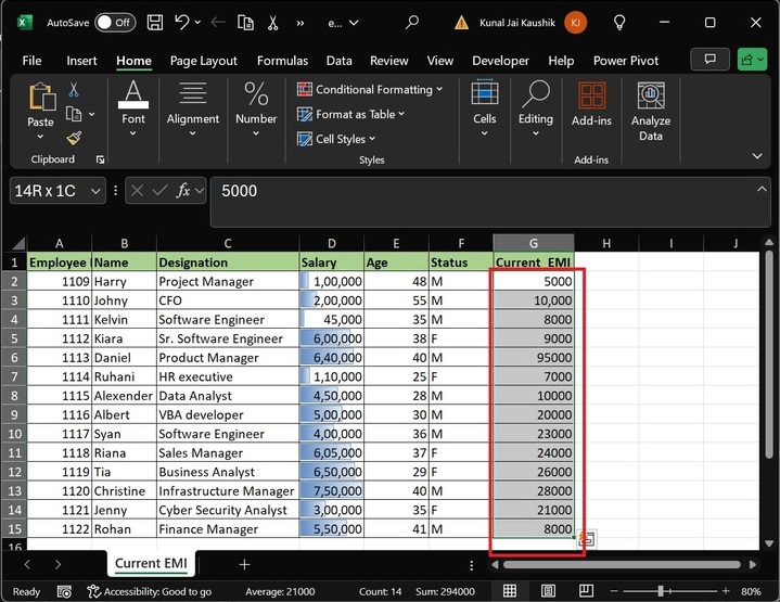
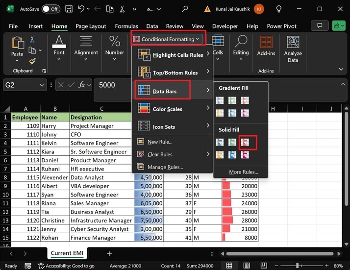
Step 2 − After that, navigate to the Home tab, select the Conditional Formatting button, choose the Data Bars option, and select the Red Data bars under the Solid Fill style.

Hence, the solid fill red data bars are added in the G column. The highest Current_EMI is 95000, as it has the longest data bars.

Custom Data Bars in Excel

You can also set your own data bar styles instead of choosing inbuilt styles. Below are the following steps −

Step 1 − Select the cell range E2:E15. Go to the "Home tab-> Conditional Formatting-> Data Bars->More Rules"

Step 2 − Another dialog box, "New Formatting Rule," will open. Select a Rule Type: "Format all cells based on their values." In the next section, "Edit the Rule Description:" select the Automatic(by default) for the minimum and maximum values. Choose the "Solid Fill" and select the green color for the Bar appearance.

Once you press the OKbutton, the green color data bar will be added to the selected range of cells.

Hide Numbers and Show Data Bars

Defined rules can be edited or deleted by using the Manage Rule. What in case if you want to display only data bars and hide the numbers. It can be possible in two ways either you can edit the existing rules or set the new rules.

Lets edit the previous section rules.

Select the cell range C2:C15 and move to the Home tab and click the Conditional Formatting and select the Manage Rules from the drop down menu.

In the "Conditional Formatting Rules Manager" dialog box, click on the "Edit Rule…" tab.

After that, select the "Show Bar Only" option under the "Edit the Rule Description" section and hit the OK.

Furthermore, click on the Apply button and hit the OKbutton.

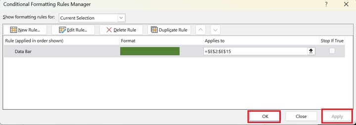
Therefore, the only Data Bars will be shown in the selected range.